Article

Temperature Forecasting Correction Based on Operational GRAPES-3km Model Using Machine Learning Methods

1
State Key Laboratory of Severe Weather and Institute of Artificial Intelligence for Meteorology, Chinese Academy of Meteorological Sciences, Beijing 100081, China
2
Baoding Meteorological Bureau, Baoding 071000, China
3
Shaanxi Meteorological Bureau, Xi’an 710014, China
4
Xiangtan Meteorological Bureau, Xiangtan 411100, China
*
Author to whom correspondence should be addressed.
Atmosphere 2022, 13(2), 362; https://doi.org/10.3390/atmos13020362
Submission received: 11 January 2022 / Revised: 15 February 2022 / Accepted: 19 February 2022 / Published: 21 February 2022

Abstract

:
Postprocess correction is essential to improving the model forecasting result, in which machine learning methods play more and more important roles. In this study, three machine learning (ML) methods of Linear Regression, LSTM-FCN and LightGBM were used to carry out the correction of temperature forecasting of an operational high-resolution model GRAPES-3km. The input parameters include 2 m temperature, relative humidity, local pressure and wind speed forecasting and observation data in Shaanxi province of China from 1 January 2019 to 31 December 2020. The dataset from September 2018 was used for model evaluation using the metrics of root mean square error (RMSE), average absolute error (MAE) and coefficient of determination (R2). All three machine learning methods perform very well in correcting the temperature forecast of GRAPES-3km model. The RMSE decreased by 33%, 32% and 40%, respectively, the MAE decreased by 33%, 34% and 41%, respectively, the R2 increased by 21.4%, 21.5% and 25.2%, respectively. Among the three methods, LightGBM performed the best with the forecast accuracy rate reaching above 84%.

1. Introduction

Numeric weather prediction has achieved good results through the accumulation of scientific knowledge, greatly improved computing power, and continuous improvement of the observation system [1]. However, due to the uncertainty of the initial field of the numerical model and its approximate treatment of the atmosphere, coupled with the random non-linear chaotic characteristics of the atmosphere [2,3], the numerical model inevitably has forecast bias [4]. The statistical post-processing method has successfully corrected many defects inherent in the prediction of numerical weather prediction models [5]. Perfect Prognostic (PP) method was proposed by Klein [6] in 1970. Then, Glahn et al. [7] proposed a Model Output Statistical (MOS) method, which became the most commonly used post-processing method. For example, it was used by Taylor et al. to assess temperature forecast error [8]; the spatial and temporal patterns of U.S. nationwide MOS forecast errors compared to individual station error trends prove to be a powerful forecasting tool for real-time forecasters, and nationwide MOS forecast error maps are useful. Combined with the field of grid analysis, Guan et al. [9] applied the Kalman filter-based decayed mean deviation estimation method to effectively improve the accuracy of temperature prediction for most of the year, with the greatest benefit from April to June, but sometimes it does not perform well when the spring and fall transition seasons are longer. Cheng and Steenburgh [10] used traditional model output statistics (ETAMOS), Kalman filter (ETAKF), 7d fixed error correction method (ETA7DBR) to correct the 2 m temperature predicted by the North American mesoscale model; ETAKF and ETA7DBR produce better predictions in the stationary cool-season mode when persistent valley and basin cold pools are present. Najafi and Moradkhani [11] used the Bayesian model averaging method to evaluate the multi-model comprehensive analysis of extreme runoff in the impact assessment of climate change. Bothwell and Richardson [12] used the perfect forecast method and logistic regression to develop equations for forecasting lightning in Alaska on a 10-km grid and in the continental United States on a 40-km grid, and these equations can be applied to NCEP model predictions. Lerch and Baran [13] used the ensemble model output statistical method for EMOS model estimation and the ‘Grand limited area model ensemble prediction system’ to predict European wind speeds. The similarity-based semi-local models proposed show significant improvement in predictive performance compared with standard regional and local estimation methods. Traditional post-processing methods are based on pre-statistical assumptions, which limits the methods to further improve the effect of model correction to a certain extent.
In recent years, with the widespread application of artificial intelligence technology in the computer field, ML technology has made remarkable achievements in many fields including atmospheric science. It has proven to be a powerful tool for identifying weather and climate patterns [14,15,16,17], improving parameterization of global circulation models [18,19,20], weather and climate prediction [21,22,23,24,25,26,27,28], and post-processing of numerical weather forecasting [29,30]. Frnda et al. [31] trained a three-layer artificial neural network (ANN) using the weather station data of eight major cities in Slovakia and the Czech Republic to improve the European Centre for Medium-Range Weather Forecasts (ECMWF) forecast output accuracy to the same level as that provided by the limited area model, and it can deliver a more accurate temperature and precipitation forecast in real-time. Bonavita et al. [32] modified the IFS model of the ECMWF with ANNS. Rasp and Lerch [33] addressed ensemble post-processing with neural network method, which significantly outperforms baseline post-processing method while being computationally more affordable in a case study of 2-m temperature prediction at a German ground station. Chapman et al. [34] used convolutional neural networks (CNN) to improve post-processing studies of the National Center for Environmental Prediction’s Global Forecast System in the field of integrated vapor transport forecasting in the eastern Pacific and western United States. This work demonstrates that CNN have the potential to improve forecasting skills for precipitation events affecting the western United States to 7 days. HAN et al. [35] used the deep learning method of CU-net to correct gridded forecasts of four weather variables from the European Centre for Medium-Range Weather Forecasting Integrated Forecast System Global Model (ECMWF-IFS): 2-m temperature, 2-m relative humidity, 10-m wind speed and 10-m wind direction. The results show that CU-net improves ECMWF-IFS forecast performance for all four weather variables for all forecast lead times from 24 h to 240 h. Li et al. [36] used the model output machine learning method (MOML) to predict 2 m surface temperature. Based on ECMWF model grid data and reanalysis field data, MOML showed better prediction performance than the ECMWF model and MOS, especially in winter. Kang et al. [37] used support vector machine (SVM)s, random forests (RF), gradient boosting decision trees (GBDT) and extreme gradient spanning tree (XGBoost) algorithms to predict 2 m temperature, relative humidity, 10 m wind speed and wind direction, and the study showed that the XGBoost method performed the best, slightly better than GBDT and random forests. The 0–10 days average prediction accuracy of 2 m relative humidity and 10 m wind speed and direction improved by nearly 15%, and the temperature accuracy improved by 20~40%. Chen and Huang [38] proposed an ensemble learning method for bias correction of station temperature forecast based on ECMWF model products and combined a new ensemble learning model (ALS model) through ANN, long short-term memory network (LSTM) and linear regression model. The correction effect is significant for the regions where the station temperature forecast error is larger and the temperature peak forecast. Cho et al. [39] used RF, Support Vector Regression (SVR), ANN, and Multi-Model Ensemble (MME) to calibrate Local Data Assimilation and Prediction System next-day model outputs for maximum and minimum air temperature, verifying the superiority of the ensemble approach. Xu et al. [40] constructed a statistical MME for deterministic and probabilistic precipitation forecasts to predict precipitation from 1 to 6 months in advance. To sum up, compared to traditional methods, ML methods are more powerful in nonlinear simulation and can often achieve higher accuracy.
The Global/Regional Assimilation and Prediction System (GRAPES) [41,42] is an operational numerical prediction model developed by the China Meteorological Administration (CMA), thus the optimization and improvement of the GRAPES model results have become important tasks in CMA for better operational forecast services. The high-resolution GRAPES-3km model especially provides essential forecasting information for highly impacted local scale weather, and the model is one of the main reference sources for province-level forecasting, which makes this study of great significance to the grass-roots forecast operation. There are several studies on the revision of the ECMWF model [35,36,38] in China areas using ML methods, but no study focused on the operational GRAPES-3km model at present. In addition, many previous studies are still in the research stage and have not been put into actual business applications. We compared and analyzed the correction effects of three ML methods on the temperature forecast of GRAPES-3km model in Shaanxi Province, and the research results have been successfully applied to the operational meteorological service guarantee of the 14th National Games with significant forecasting improvement.

2. Model Forecast and Observation Data

The GRAPES-3km model forecasting data from 1 January 2019 to 31 December 2020 were used for correction post-processing, with a time span of 731 days. The temporal and spatial resolution of the model are 1 h and 0.03° (about 3 km), respectively. The model starts twice a day at 00:00 (UTC) and 12:00 (UTC). A total of 37 forecast timeliness of 0–36 h (hourly increments) was selected. For each forecast timeliness, the model produces two forecast results every day, with a sample size of (731 × 2). The contemporaneous surface observation data of 293 meteorological stations in Shaanxi Province (Figure 1) comes from the data-sharing platform of the Chinese Academy of Meteorological Sciences.
Temperature is mainly related to meteorological factors such as air pressure, humidity and wind that reflect the state of the atmosphere. So, several elements of the model products were selected, including 2 m air temperature, 10 m wind U and V components, local pressure and relative humidity; the wind speed value was calculated from U and V components.
During the 14th National Games in China, the GRAPES-3km model data and observation data from 1 September to 26 September 2021 were used to conduct operational practical tests on the overall performance of the model.

3. Data Preprocessing

The outlier values of the observation data were detected with three times the standard deviation and removed. The missing values were filled by linear interpolation to form a more precise and complete observation dataset.
The GRAPES-3km model forecast outputs are grid point data. First, the outlier samples exceeding climate extreme values of the model data were removed, and then the model data were interpolated to the positions of 293 sites using the inverse distance weighting (IDW) method.
Each sample consists of observational data, model forecast data and station location information. The observation data include the 48 hourly four elements of air pressure, wind speed, relative humidity, and temperature before the forecast time, which were arranged in the order from early to later to form the observation time series. The model forecast data also include the four elements with a time range of 12 h before the forecast leading time. If the forecast leading time is less than 12 h, the time range includes 0 to the leading time hour. The model data were also arranged in chronological order from early to later. Station location information includes station longitude, latitude, and altitude. The three kinds of data are combined into a complete data sample in sequence. Because there are 37 prediction time periods (0 to 36 h), in total, 37 ML models were trained with the sample datasets for each ML method, respectively.
The data need to be standardized before inputting to the ML model for two methods of linear regression and LSTM-FCN, which was performed with the Python ML package scikit-learn. The bottom layer of the LightGBM model is based on a decision tree. The decision tree enters different branches according to the value of the feature, and each feature is independent of each other. Unlike the neuron of the neural network, which accumulates each input signal, the LightGBM model does not need to standardize the input features, which is more convenient for usage.

4. Methods and Modeling

In this study, three machine learning methods of Linear Regression, Long-Short Term Memory Fully Convolutional Network (LSTM-FCN) [43] and LightGBM [44] were used to study the 2 m air temperature prediction of the GRAPES-3km model. These three methods were selected for comparing the correction effects of traditional ML methods and deep learning methods on the model. Linear Regression performs a regression task using least square function to model the relationship between one or more independent variables and dependent variables. This function is a linear combination of one or more model parameters called regression coefficients. There is an epidemiological example to predict disease and velocity of COVID-2019 cases in India using linear regression by Sujath et al. [45]. Wang et al. [46] used the linear regression method to study the temperature correction in Shaanxi Province. Linear regression method outperforms other methods in short-term forecasting [36]. On the one hand, numerical model forecast does not deviate very much from short-term predictions, so a linear relationship can be established, which is well applied between its output and observations. It is also the simplest ML method, fast to compute, and works well in many situations. Its disadvantage is that it does not fit nonlinear data well. The linear regression method was implemented using scikit-learn.
Long Short-Term Memory Fully Convolutional Network (LSTM-FCN) have received widespread attention over the past decade for their ability to successfully model nonlinear feature interactions [47]. Long Short-Term Memory (LSTM) [48] is an extension of recurrent neural networks (RNN) with capable of learning long-term dependencies. It has a cell state and three gates of forget gate, input gate and output gate which provides them with the power to selectively learn, unlearn or retain information from each of the units. It is widely used in time series problems, which are naturally associated with meteorological data. This study attempts to use LSTM to mine the time series association between observation data and forecast elements. The limitation of LSTM networks is that they can only take time series data as input. If LSTM is used alone, it is impossible to combine site weather element forecast and site location information. To solve this problem, LSTM-FCN was chosen. LSTM-FCN is a time-series-based multivariate LSTM full convolutional network that has the capability to successfully model nonlinear feature interactions. Through the FCN layer, the time series information mined by LSTM, the forecast of meteorological elements of the site, as well as the altitude, latitude and longitude information of the site are combined. Karim et al. [43] mentioned that the proposed LSTM-FCN achieves state-of-the-art performance compared to others. The Keras framework was used to implement the LSTM-FCN method. The input of the LSTM model is the air pressure, relative humidity, wind speed and temperature of the observation station in the past 48 h, splicing 4 × i eigenvalues (the pressure, temperature, humidity and wind speed of the ith prediction time of the GRAPES-3km model, the value of i is 0–12) to form a time series (sample size, 4 × (48 + i)), after two LSTM layers (the number of LSTM units are 256 and 64, respectively), the output is spliced 7 eigenvalues (the pressure, temperature, humidity, wind speed at the current forecast time of GRAPES-3km model and station latitude, longitude and altitude) and then connect two fully connected layers (the number of neurons is 256 and 32, respectively, and the activation function is ReLU) to obtain the final result. For example, at time 0, the LSTM-FCN stitching layer has 4 × 48 + 7 = 199 eigenvalues, and at time 13, the LSTM-FCN stitching layer has 4 × 60 + 7 = 243 eigenvalues. The structure diagram of the LSTM-FCN model at time 0 is predicted, as shown in Figure 2. The optimizer is Adam, and the initial learning rate is set to 0.3 × 10⁻⁴.
LightGBM is widely used [49,50,51], and has the advantages of high accuracy, less overfitting and a fast training speed. Ke [30] mentioned that LightGBM speeds up the training process of traditional GBDT by more than 20 times, while achieving almost the same accuracy. LightGBM is a gradient boosting framework that uses tree-based learning algorithms. It is designed to be distributed and enables highly efficient training across large-scale datasets with low memory cost by implementing two novel techniques of gradient-based one-sided sampling and exclusive feature bundling. It is a variant of the decision tree and is based on a histogram algorithm. The basic idea is discretizing successive floating-point eigenvalues into k integers, and at the same time constructing a histogram with a width of k. When traversing data, the statistics are accumulated in the histogram based on the discretized values as indexes, and when the data are traversed once, the histogram accumulates the required statistics, and then according to the discrete values of the histogram, iterates to find the optimal segmentation point. Because LightGBM only supports two-dimensional structured datasets, each sample in the dataset is the LightGBM input feature sequence. This study uses the Python environment to import the LightGBM package to achieve. The schematic diagram of the correction method of LightGBM is shown in Figure 3.
We used the GridSearchCV function of scikit-learn to adjust the parameters of LightGBM to obtain the optimal parameter settings. Through the parameter test, the parameter list is obtained, as seen in Table 1. The parameters of the LightGBM model are initialized to obtain the final training result.

5. Verification Scores

RMSE, MAE, R2 and the forecast accuracy rate scores were used to evaluate the forecast correction effects.
The RMSE is the square root of the ratio of the sum of the squares of the deviation between the forecasting value and the true value to the number of observations. It is used to measure the deviation between the forecasted value and the true value. The smaller the RMSE value, the higher the forecast accuracy.
RMSE = 1 n i = 1 n ( y i y ^ i ) 2
where y ^ i is the predicted value, and y i is the observation value.
The MAE is the average value of the absolute error, which can better reflect the actual situation of the predicted value error.
MAE = 1 n i = 1 n | y i y ^ i |
R2 is the coefficient of determination (goodness of fit), which reflects the proportion of the dependent variable that can be explained by the independent variable through the regression relationship. When R2 = 1, the predicted value and the true value in the sample are the same without any error. If R2 = 0, the numerator is equal to the denominator, and each predicted value of the sample is equal to the mean. R2 is not the square of r, it may also be a negative number (numerator > denominator).
R 2 ( y , y ^ ) = 1 i = 0 n 1 ( y i y ^ i ) 2 i = 0 n 1 ( y i y ¯ i ) 2

6. Results

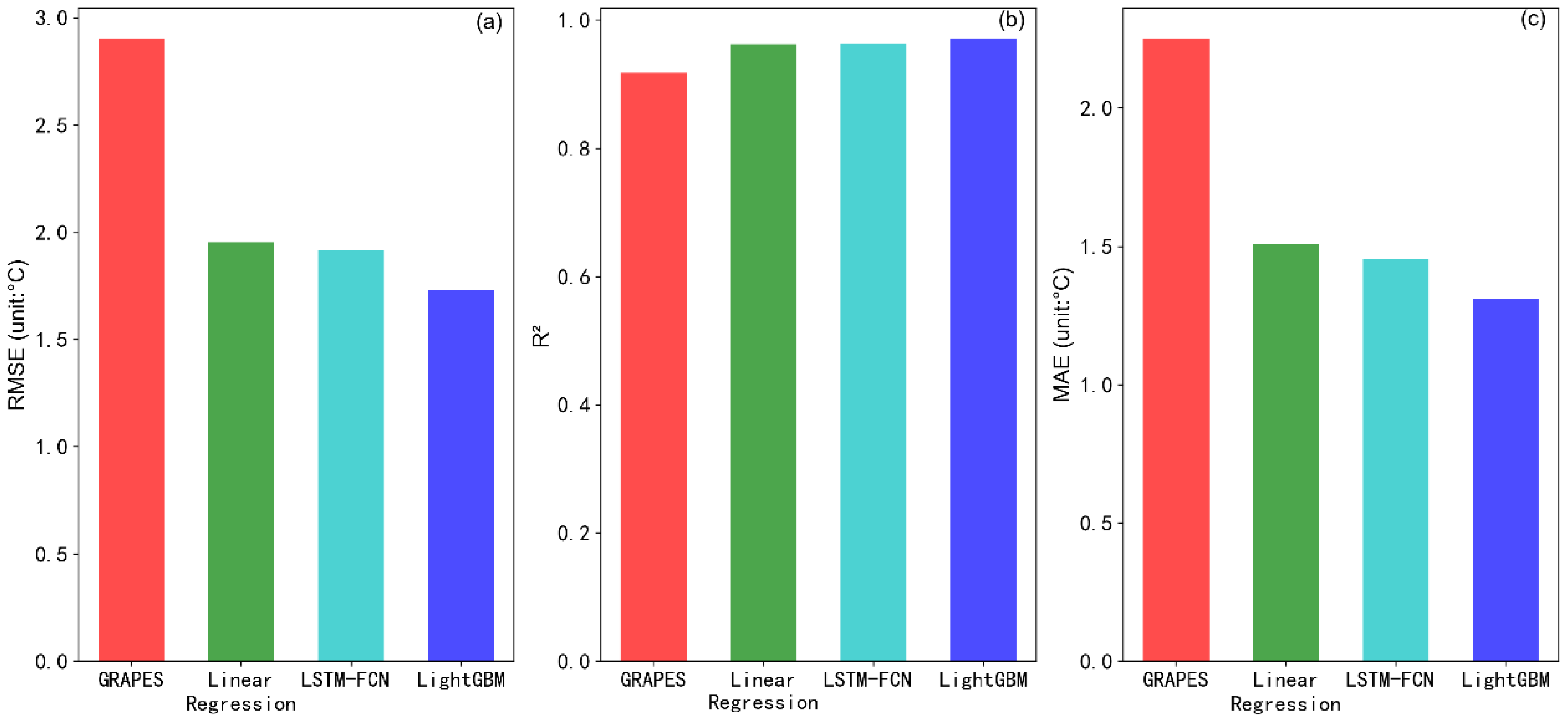
In order to more accurately reflect the distribution characteristics of the overall data in the training set and validate set, we extracted the validate set every 5 days from the two years dataset, and the rest was used as training set. Three methods of Linear Regression, LSTM-FCN and LightGBM were used to train and validate the dataset, and the results were scored. As shown in Figure 4, the average RMSE of the GRAPES-3km model forecast for 37 timeliness is 2.90 °C. For linear regression, the correction improvement rate of RSTM is about 33% to the value of 1.95 °C. The RMSE improvement rate of LSTM-FCN correction is about 34% to the value of 1.92 °C. LightGBM method performs the best with the RMSE value of 1.48 °C and the improvement rate of 40%. The MAE of the GRAPES-3km model, Linear Regression, LSTM-FCN and LightGBM are 2.25 °C, 1.30 °C, 1.29 °C, and 1.14 °C, respectively. The R2 values of the model output and three correction methods reached 0.96 or higher.
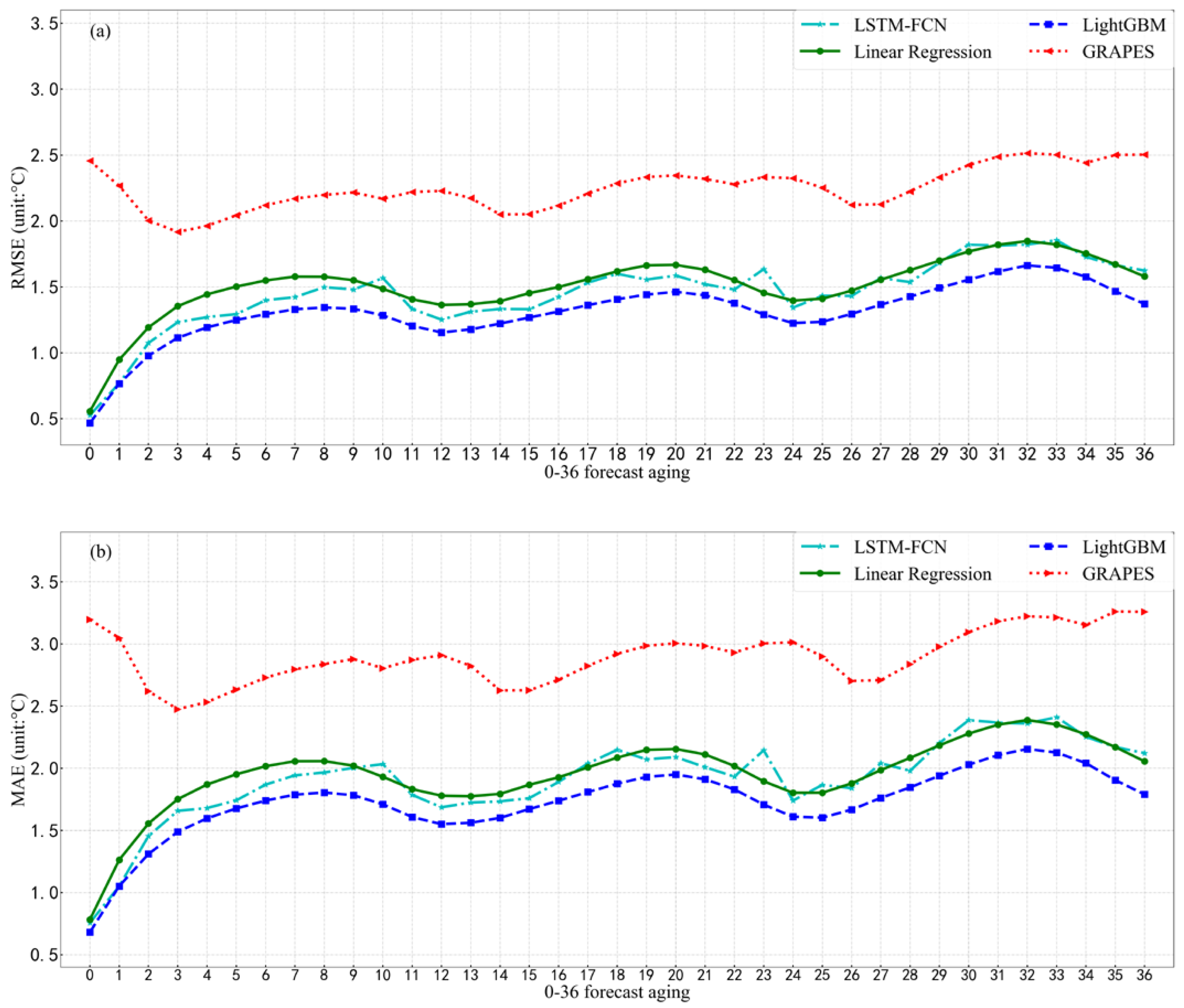
In the distribution of the RMSE and MAE from 0 to 36 h forecast timelines (Figure 5), the correction results of Linear Regression, LSTM-FCN and LightGBM are affected by the GRAPES-3km model output. The RMSE and MAE were basically consistent with the change trend of GRAPES-3km model except for the initial 3 h, showing a trend of alternating troughs and crests, and the overall trend of prolonged forecasting effect with time effect is decreasing.
The model and observation data of September 2018 were used as a test set to test the correction performance of the three methods of Linear Regression, LSTM-FCN and LightGBM. The overall average RMSE and MAE results are shown in Table 2, the RMSE of 0–36 h forecast by GRAPES-3km model are all greater than 2.0 °C with an average value of 2.472 °C. The RMSE values of the 0–36 h of the Linear Regression correction are between 0.78–1.97 °C with an average value of 1.665 °C. The RMSE values of the 0–36 h of the LSTM-FCN correction are 0.70–2.26 °C with an average value of 1.689 °C. The RMSE values of the LightGBM correction are 0.62–1.84 °C with an average value of 1.485 °C. The RMSE improvement rates of the three correction methods are 32.6%, 32.1% and 39.9%, respectively. The overall correction performance according to RMSE, from best to worst, is LightGBM, LSTM-FCN and Linear Regression. For the MAE, an average values of the GRAPES-3km mode, Linear Regression, LSTM-FCN and LightGBM are 1.946 °C, 1.299 °C, 1.288 °C and 1.140 °C, respectively. The improvement rates of MAE of the three correction methods are 33.3%, 33.8%, and 41.4%, respectively.
In operational weather forecasting, the accuracy of temperature forecast is judged by using the difference between the forecast result and the actual value not greater than 2.0 °C, that is, the forecast is judged to be correct, otherwise the forecast is wrong.
accuracy = c o u n t ( | T p r e d T r e a l | 2.0 ) c o u n t ( T r e a l ) × 100 %
where, T p r e d is the predicted value of temperature, and Treal is the actual value. The accuracy test results at 293 stations in September 2018 were calculated to verify the model forecast and the correction performance for each station. The spatial distribution of forecast accuracy values is plotted in Figure 6. For the GRAPES-3km model, accuracy varies widely from station to station, and there are 154 stations with forecast accuracy of more than 60%. After correction by the Linear Regression method, the accuracy values of all stations are above 60%, and there are 135 stations with accuracies of more than 80%. The forecast accuracy values are improved by more than 30% in 143 stations compared with the model output. For LSTM-FCN method, the accuracy values of all stations are more than 64%, and there are 141 stations that are more than 80%. LightGBM has the best correction effect, with an accuracy of more than 80% at 250 stations; there are 130 stations more than 85%, and the accuracy values are improved by more than 30% at 170 stations.
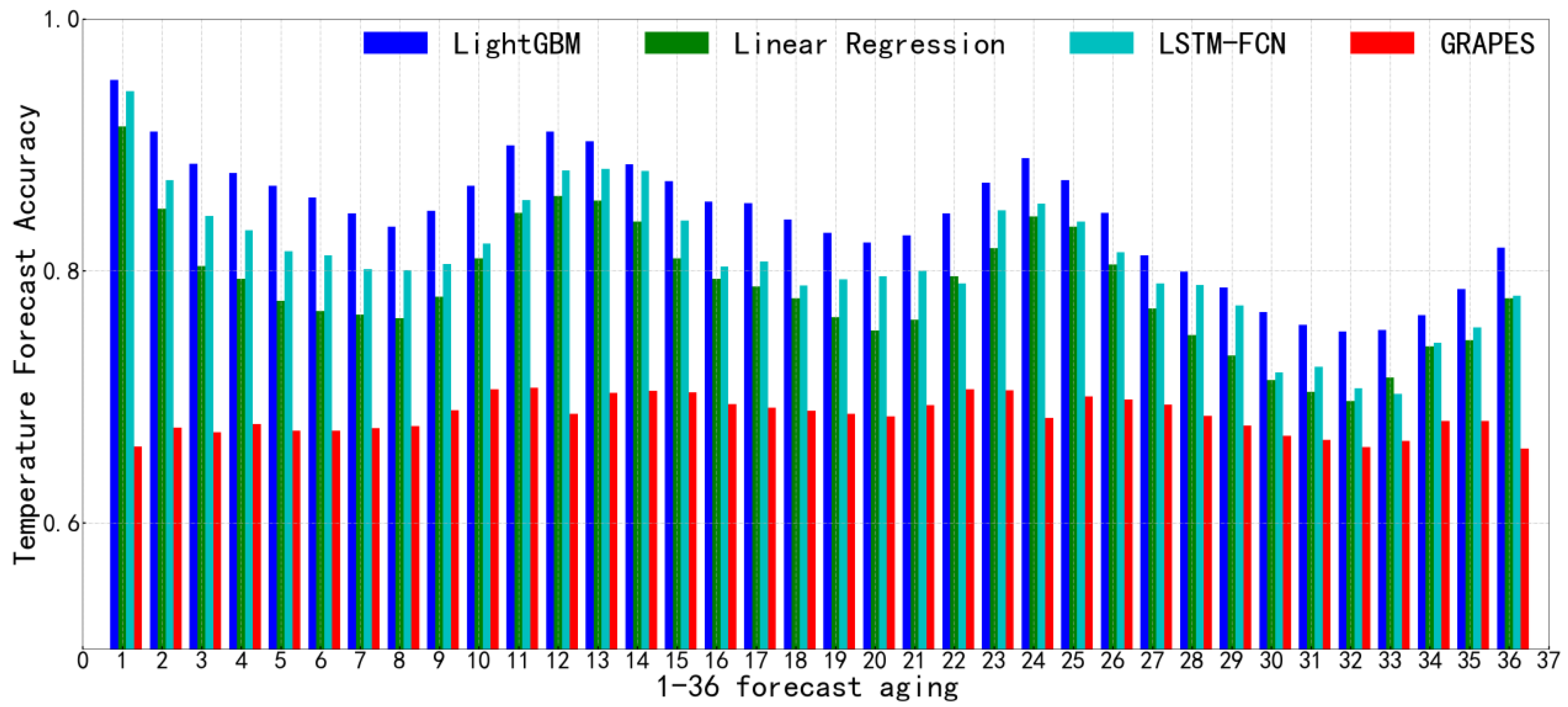
Using the research results, during the 14th National Games, we used the LightGBM model to correct the temperature forecast and improve the forecast skills. The average RMSE of 36 time periods is 2.356 for GRAPES-3km model and 1.526 for LightGBM correction; the RMSE decreases 35.2%. The average MAE of GRAPES-3km model is 1.725, and the value is 1.143 after correction by LightGBM, with the MAE decreasing by 33.7%. The forecast accuracy of GRAPES-3km model is 68.4% and the value is 84.1% after correction, with the forecast accuracy increasing by 23%. The comparison results of the temperature forecast accuracy of the three methods during the 14th National Games, as shown in Figure 7.

7. Conclusions and Discussion

Three machine learning methods of Linear Regression, LSTM-FCN and LightGBM were used to revise and compare the temperature forecast of the GRAPES-3km model in Shaanxi Province of China. RMSE, MAE, R2 and forecast accuracy were used as the evaluation metrics. After correction by the three methods, the RMSE values decreased by 33%, 32%, and 40%, and the MAE values decreased by 33%, 34% and 41%, and the R2 values increased by 21.4%, 21.5% and 25.2%, respectively. All three machine learning methods perform well, with forecast accuracies of more than 78%. Among them, LightGBM has the best performance with a forecast accuracy of more than 84%.
It can be seen from the change curve of RMSE and MAE for 0–36 h forecast, the three methods are affected by the forecast temperature variation of the GRAPES-3km model, and the forecast correction metrics become worse with the extension of forecast timelines. LightGBM has the best correction performance at all forecast timelines.
The sample data volume in this study is large with each aging hour sample size reaching 50,000, which can fully characterize the evolution of temperature and reduce the probability of overfitting of the model. The past 48 h of temperature observation data were used, so the daily changes and weather system evolution can be extracted by the machine learning methods. In addition, the meteorological elements of the air pressure, wind speed and relative humidity that are highly correlated with the temperature were used to help learn more related information. The location information of the stations can reduce the error from the spatial and altitude difference of stations.
The LightGBM method is slightly better than the other two methods. It has the characteristics of feature parallelism and data parallelism and has the ability to find the best cut points (features and thresholds) according to the assigned feature set, which help to filter out the feature parameters that have a significant impact on the forecast results. In the model prediction, the characteristics with large weight coefficients are given a higher degree of participation, which can better reflect the changing characteristics of meteorological elements. The method was applied to the meteorological forecast service of the 14th National Games of China and performed well with an average forecast accuracy rate of 36 h reaching 84.1%.

Author Contributions

Conceptualization, Y.W. and H.Z.; Data curation, H.Z. and Y.W.; formal analysis, H.Z.; visualization, H.Z.; funding acquisition, Y.W.; investigation, H.Z., X.Y. and D.C.; methodology, H.Z., Y.W., D.C., D.F. and W.W.; writing—original draft, H.Z.; writing—review and editing, Y.W. and D.C. All authors have read and agreed to the published version of the manuscript.

Funding

This research was supported by grants from the NSFC Major Project (42090030), the National Key Research and Development Program (2019YFC0214601), and the CAMS project (2020Z011).

Institutional Review Board Statement

Not applicable.

Informed Consent Statement

Not applicable.

Data Availability Statement

Restrictions apply to the availability of these data. Data was obtained from CMA and are available from the corresponding authors with the permission of CMA.

Acknowledgments

We acknowledge support from the above funding projects.

Conflicts of Interest

The authors declare no conflict of interest.

References

  1. Bauer, P.; Thorpe, A.; Brunet, G. The quiet revolution of numerical weather prediction. Nature 2015, 525, 47–55. [Google Scholar] [CrossRef] [PubMed]
  2. Lorenz, E.N. Deterministic Nonperiodic Flow. J. Atmos. Sci. 1963, 20, 130–141. [Google Scholar] [CrossRef] [Green Version]
  3. Slingo, J.; Palmer, T. Uncertainty in weather and climate prediction. Philos. Trans. R. Soc. A Math. Phys. Eng. Sci. 2011, 369, 4751–4767. [Google Scholar] [CrossRef]
  4. Cui, B.; Toth, Z.; Zhu, Y.; Hou, D. Bias correction for global ensemble forecast. Weather Forecast. 2012, 27, 396–410. [Google Scholar] [CrossRef]
  5. Prog, P.; Marzban, C.; Sandgathe, S.; Kalnay, E. MOS, Perfect Prog, and Reanalysis. Mon. Weather Rev. 2005, 134, 657–663. [Google Scholar]
  6. Klein, W.H.; Lewis, F. Computer Forecasts of Maximum and Minimum Temperatures. J. Appl. Meteorol. Climatol. 1970, 9, 350–359. [Google Scholar] [CrossRef] [Green Version]
  7. Glahn, H.R.; Lowry, D.A. The Use of Model Output Statistics (MOS) in Objective Weather Forecasting. J. Appl. Meteorol. Climatol. 1972, 11, 1203–1211. [Google Scholar] [CrossRef] [Green Version]
  8. Taylor, A.A.; Leslie, L.M. A Single-Station Approach to Model Output Statistics Temperature Forecast Error Assessment. Weather Forecast. 2005, 20, 1006–1020. [Google Scholar] [CrossRef]
  9. Guan, H.; Cui, B.; Zhu, Y. Improvement of statistical postprocessing using GEFS reforecast information. Weather Forecast. 2015, 30, 841–854. [Google Scholar] [CrossRef]
  10. Cheng, W.Y.Y.; Steenburgh, W.J. Strengths and weaknesses of MOS, running-mean bias removal, and Kalman filter techniques for improving model forecasts over the western United States. Weather Forecast. 2007, 22, 1304–1318. [Google Scholar] [CrossRef]
  11. Najafi, M.R.; Hamid, M. Multi-Model Ensemble Analysis of Runoff Extremes for Climate Change Impact Assessments. J. Hydrol. 2015, 525, 352–361. [Google Scholar] [CrossRef] [Green Version]
  12. Bothwell, P.D.; Richardson, L.M. Forecasting lightning using a perfect prog technique applied to multiple operational models. Int. Conf. Atmos. Electr. ICAE 2014, 2014, 15–20. [Google Scholar]
  13. Lerch, S.; Baran, S. Similarity-based semilocal estimation of post-processing models. J. R. Stat. Soc. Ser. C Appl. Stat. 2017, 66, 29–51. [Google Scholar] [CrossRef]
  14. Barnes, E.A.; Hurrell, J.W.; Ebert-Uphoff, I.; Anderson, C.; Anderson, D. Viewing Forced Climate Patterns Through an AI Lens. Geophys. Res. Lett. 2019, 46, 13389–13398. [Google Scholar] [CrossRef] [Green Version]
  15. Toms, B.A.; Kashinath, K.; Prabhat; Yang, D. Testing the reliability of interpretable neural networks in geoscience using the Madden-Julian oscillation. Geosci. Model Dev. 2021, 14, 4495–4508. [Google Scholar] [CrossRef]
  16. Barnes, E.A.; Toms, B.; Hurrell, J.W.; Ebert-Uphoff, I.; Anderson, C.; Anderson, D. Indicator Patterns of Forced Change Learned by an Artificial Neural Network. J. Adv. Model. Earth Syst. 2020, 12, e2020MS002195. [Google Scholar] [CrossRef]
  17. Watt-Meyer, O.; Brenowitz, N.D.; Clark, S.K.; Henn, B.; Kwa, A.; McGibbon, J.; Perkins, W.A.; Bretherton, C.S. Correcting Weather and Climate Models by Machine Learning Nudged Historical Simulations. Geophys. Res. Lett. 2021, 48, e2021GL092555. [Google Scholar] [CrossRef]
  18. Rasp, S.; Pritchard, M.S.; Gentine, P. Deep learning to represent subgrid processes in climate models. Proc. Natl. Acad. Sci. USA 2018, 115, 9684–9689. [Google Scholar] [CrossRef] [Green Version]
  19. Yuval, J.; O’Gorman, P.A.; Hill, C.N. Use of Neural Networks for Stable, Accurate and Physically Consistent Parameterization of Subgrid Atmospheric Processes With Good Performance at Reduced Precision. Geophys. Res. Lett. 2021, 48, e2020GL091363. [Google Scholar] [CrossRef]
  20. Brenowitz, N.D.; Bretherton, C.S. Spatially Extended Tests of a Neural Network Parametrization Trained by Coarse-Graining. J. Adv. Model. Earth Syst. 2019, 11, 2728–2744. [Google Scholar] [CrossRef] [Green Version]
  21. Ham, Y.G.; Kim, J.H.; Luo, J.J. Deep learning for multi-year ENSO forecasts. Nature 2019, 573, 568–572. [Google Scholar] [CrossRef] [PubMed]
  22. Ko, C.M.; Jeong, Y.Y.; Lee, Y.M.; Kim, B.S. The development of a quantitative precipitation forecast correction technique based on machine learning for hydrological applications. Atmosphere 2020, 11, 111. [Google Scholar] [CrossRef] [Green Version]
  23. Anderson, G.J.; Lucas, D.D. Machine Learning Predictions of a Multiresolution Climate Model Ensemble. Geophys. Res. Lett. 2018, 45, 4273–4280. [Google Scholar] [CrossRef]
  24. Krasnopolsky, V.M.; Lin, Y. A neural network nonlinear multimodel ensemble to improve precipitation forecasts over continental US. Adv. Meteorol. 2012, 2012, 649450. [Google Scholar] [CrossRef]
  25. Kumar, A.; Mitra, A.K.; Bohra, A.K.; Iyengar, G.R.; Durai, V.R. Multi-model ensemble (MME) prediction of rainfall using neural networks during monsoon season in India. Meteorol. Appl. 2012, 19, 161–169. [Google Scholar] [CrossRef]
  26. Weyn, J.A.; Durran, D.R.; Caruana, R. Can Machines Learn to Predict Weather? Using Deep Learning to Predict Gridded 500-hPa Geopotential Height from Historical Weather Data. J. Adv. Model. Earth Syst. 2019, 11, 2680–2693. [Google Scholar] [CrossRef]
  27. Li, Y.; Liang, Z.; Hu, Y.; Li, B.; Xu, B.; Wang, D. A multi-model integration method for monthly streamflow prediction: Modified stacking ensemble strategy. J. Hydroinform. 2020, 22, 310–326. [Google Scholar] [CrossRef]
  28. Farchi, A.; Laloyaux, P.; Bonavita, M.; Bocquet, M. Using machine learning to correct model error in data assimilation and forecast applications. Q. J. R. Meteorol. Soc. 2021, 147, 3067–3084. [Google Scholar] [CrossRef]
  29. Yu, C.; Ahn, H.; Seok, J. Coordinate-RNN for error correction on numerical weather prediction. In Proceedings of the 2018 International Conference on Electronics, Information, and Communication (ICEIC), Honolulu, HI, USA, 24–27 January 2018; pp. 1–3. [Google Scholar]
  30. Kim, H.; Ham, Y.G.; Joo, Y.S.; Son, S.W. Deep learning for bias correction of MJO prediction. Nat. Commun. 2021, 12, 3087. [Google Scholar] [CrossRef]
  31. Frnda, J.; Durica, M.; Nedoma, J.; Zabka, S.; Martinek, R.; Kostelansky, M. A weather forecast model accuracy analysis and ecmwf enhancement proposal by neural network. Sensors 2019, 19, 5144. [Google Scholar] [CrossRef] [Green Version]
  32. Bonavita, M.; Laloyaux, P. Machine Learning for Model Error Inference and Correction. J. Adv. Model. Earth Syst. 2020, 12, e2020MS002232. [Google Scholar] [CrossRef]
  33. Rasp, S.; Lerch, S. Neural networks for postprocessing ensemble weather forecasts. Mon. Weather Rev. 2018, 146, 3885–3900. [Google Scholar] [CrossRef] [Green Version]
  34. Chapman, W.E.; Subramanian, A.C.; Delle Monache, L.; Xie, S.P.; Ralph, F.M. Improving Atmospheric River Forecasts with Machine Learning. Geophys. Res. Lett. 2019, 46, 10627–10635. [Google Scholar] [CrossRef]
  35. Han, L.; Chen, M.; Chen, K.; Chen, H.; Zhang, Y.; Lu, B.; Song, L.; Qin, R. A Deep Learning Method for Bias Correction of ECMWF 24–240 h Forecasts. Adv. Atmos. Sci. 2021, 38, 1444–1459. [Google Scholar] [CrossRef]
  36. Li, H.; Yu, C.; Xia, J.; Wang, Y.; Zhu, J.; Zhang, P.; Li, H.C.; Yu, C.; Xia, J.J.; Wang, Y.C.; et al. A Model Output Machine Learning Method for Grid Temperature Forecasts in the Beijing Area. Adv. Atmos. Sci. 2019, 36, 1156–1170. [Google Scholar] [CrossRef]
  37. Yanyan, K.; Haochen, L.; Jiangjiang, X.; Yingxin, Z. Post-processing for NWP Outputs Based on Machine Learning for 2022 Winter Olympics Games over Complex Terrain. EGU Gen. Assem. 2020, 2020, 10463. [Google Scholar]
  38. Chen, Y.W.; Huang, X.M.; Li, Y.; Chen, Y.; Tsui, C.; Huang, X. Ensemble Learning for Bias Correction of Station Temperature Forecast Based on ECMWF Products. J. Appl. Meteorol. Sci. 2020, 31, 494–503. [Google Scholar]
  39. Cho, D.; Yoo, C.; Im, J.; Cha, D.H. Comparative Assessment of Various Machine Learning-Based Bias Correction Methods for Numerical Weather Prediction Model Forecasts of Extreme Air Temperatures in Urban Areas. Earth Space Sci. 2020, 7, e2019EA000740. [Google Scholar] [CrossRef] [Green Version]
  40. Xu, L.; Chen, N.; Zhang, X.; Chen, Z. A data-driven multi-model ensemble for deterministic and probabilistic precipitation forecasting at seasonal scale. Clim. Dyn. 2020, 54, 3355–3374. [Google Scholar] [CrossRef]
  41. Shen, X.S.; Chen, Q.Y.; Sun, J.; Han, W.; Gong, J.D.; Li, Z.C.; Wang, J.J. Development of Operational Global Medium-Range Forecast System in National Meteorological Centre. Meteor Mon. 2021, 47, 645–654. [Google Scholar]
  42. Shen, X.S.; Su, Y.; Hu, J.L.; Wang, J.C.S. Development and Operation Transformation of GRAPES Global Middle-range Forecast System. J. Appl. Meteorol. Sci. 2017, 28, 1–10. [Google Scholar]
  43. Karim, F.; Majumdar, S.; Darabi, H.; Chen, S. LSTM Fully Convolutional Networks for Time Series Classification. IEEE Access 2018, 6, 1662–1669. [Google Scholar] [CrossRef]
  44. Ke, G.; Meng, Q.; Finley, T.; Wang, T.; Chen, W.; Ma, W.; Ye, Q.; Liu, T. LightGBM: A Highly Efficient Gradient Boosting Decision Tree. Adv. Neural Inf. Process. Syst. 2017, 30, 1–9. [Google Scholar]
  45. Sujath, R.; Chatterjee, J.M.; Hassanien, A.E. A machine learning forecasting model for COVID-19 pandemic in India. Stoch. Environ. Res. Risk Assess. 2020, 34, 959–972. [Google Scholar] [CrossRef] [PubMed]
  46. Wang, D.; Wang, J.P.; Bai, Q.M.; Gao, H.Y. Comparative correction of air temperature forecast from ECMWF Model by the decaying averaging and the simple linear regression methods. Meteor Mon. 2019, 45, 1310–1321. [Google Scholar]
  47. Ortego, P.; Diez-Olivan, A.; Del Ser, J.; Veiga, F.; Penalva, M.; Sierra, B. Evolutionary LSTM-FCN networks for pattern classification in industrial processes. Swarm Evol. Comput. 2020, 54, 100650. [Google Scholar] [CrossRef]
  48. Hochreiter, S. Long Short-term Memory. Neural Comput. 2016, 9, 1735–1780. [Google Scholar] [CrossRef]
  49. Wang, Y.; Wang, T. Application of improved LightGBM model in blood glucose prediction. Appl. Sci. 2020, 10, 3227. [Google Scholar] [CrossRef]
  50. Zhang, J.; Mucs, D.; Norinder, U.; Svensson, F. LightGBM: An Effective and Scalable Algorithm for Prediction of Chemical Toxicity-Application to the Tox21 and Mutagenicity Data Sets. J. Chem. Inf. Model. 2019, 59, 4150–4158. [Google Scholar] [CrossRef]
  51. Gan, M.; Pan, S.; Chen, Y.; Cheng, C.; Pan, H.; Zhu, X. Application of the machine learning lightgbm model to the prediction of the water levels of the lower columbia river. J. Mar. Sci. Eng. 2021, 9, 496. [Google Scholar] [CrossRef]
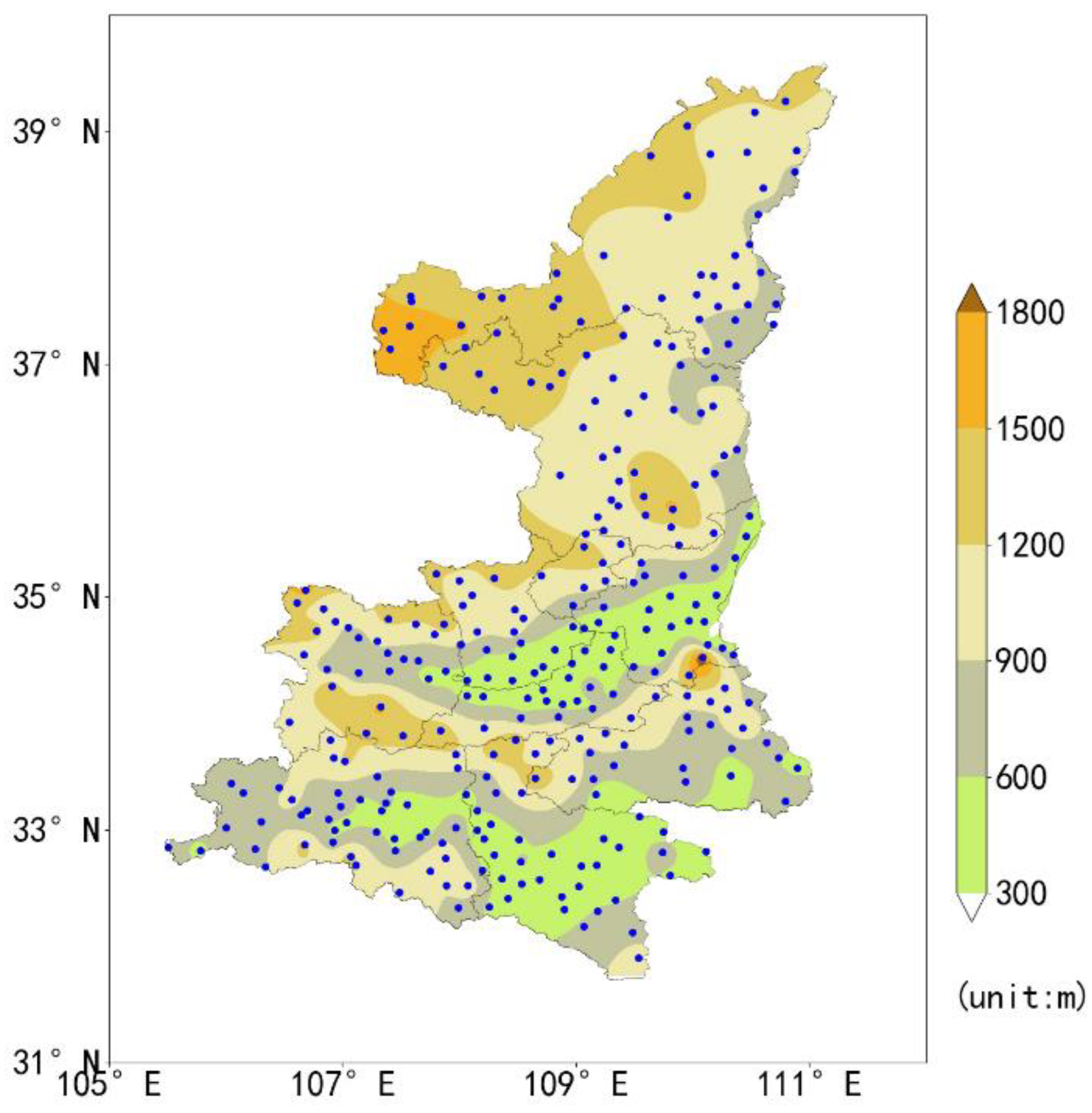
Figure 1. Research area of Shannxi Province and the distribution of observation stations. The shaded color represents the relief elevation.
Atmosphere 13 00362 g001
Figure 2. Structure diagram of LSTM-FCN model for predicting 0 aging.
Atmosphere 13 00362 g002
Figure 3. Schematic diagram of LightGBM correction method.
Atmosphere 13 00362 g003
Figure 4. Averaged RMSE (a), R2 (b) and MAE (c) values of the GRAPES-3km model and the three correction methods.
Atmosphere 13 00362 g004
Figure 5. RMSE (a) and MAE (b) values of the GRAPES-3km model and the three correction methods at forecast timelines from 0 to 36 h.
Atmosphere 13 00362 g005
Figure 6. Spatial distribution of forecast accuracy from the model and three correction methods.
Atmosphere 13 00362 g006
Figure 7. Comparison of the correction effects of the three methods for 1–36-h temperature forecast accuracy.
Atmosphere 13 00362 g007
Table 1. LightGBM model core parameters.
Learning rate0.03
Boost typeGBDT
Max depth5
Num leaves120
ObjectiveRegression_12
Feature fraction0.8
Bagging fraction0.9
Bagging freq5
Table 2. Overall average temperature forecast scores and improvement rates from the correction methods in September 2018.
ModelRMSERMSE Correction Improvement RateR2R2 Correction Improvement RateMAEMAE Correction Improvement Rate
GRAPES-3km2.472 -0.721-1.946 -
Linear Regression1.665 0.326 0.8770.2161.299 0.333
LSTM-FCN1.679 0.321 0.876 0.2141.288 0.338
LightGBM1.4850.399 0.903 0.2521.140 0.414
Publisher’s Note: MDPI stays neutral with regard to jurisdictional claims in published maps and institutional affiliations.