
Bandung Rainfall Forecast and Its Relationship with Niño 3.4 Using Nonlinear Autoregressive Exogenous Neural Network

 ,
,  , , and
Abstract
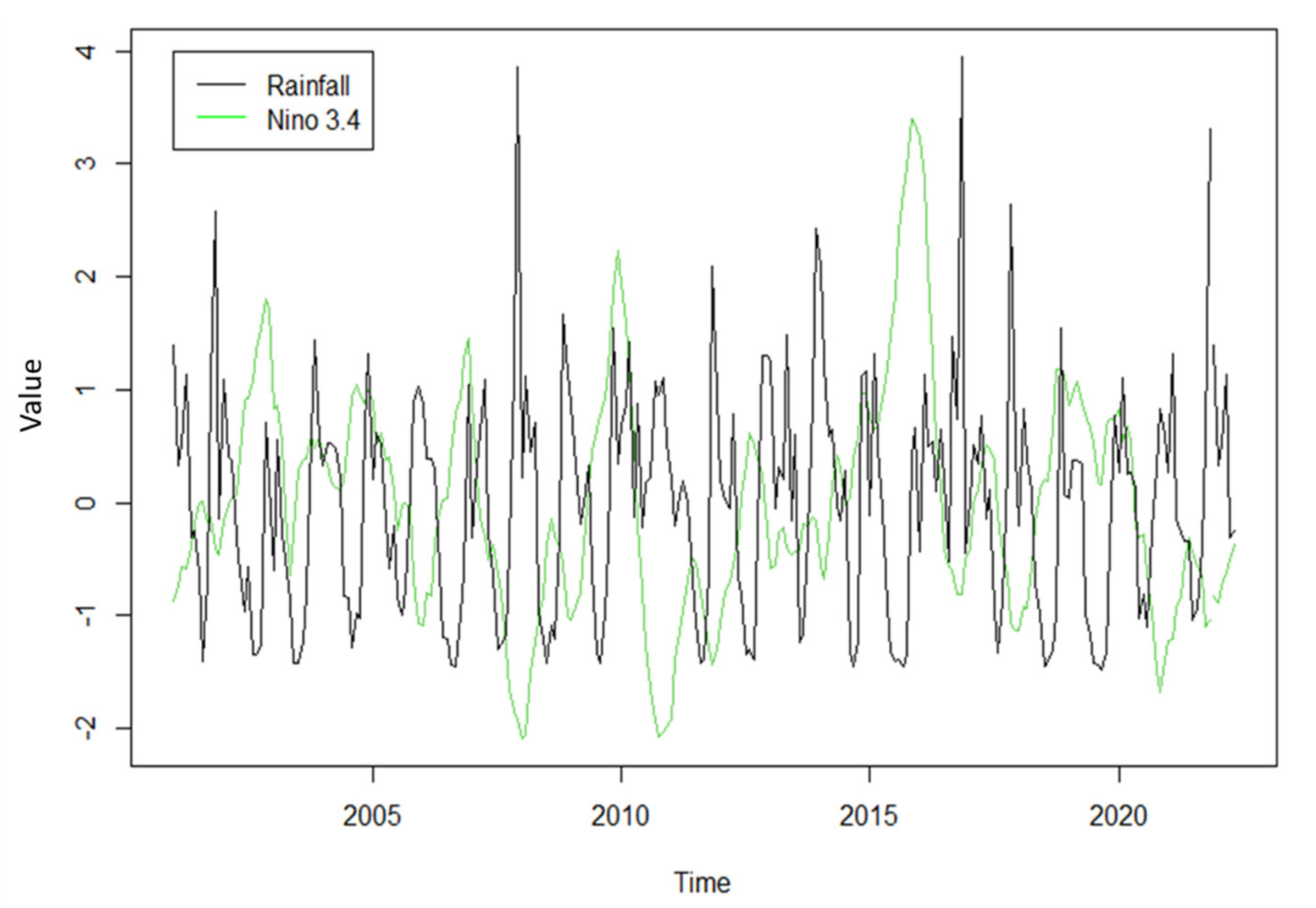
:1. Introduction
2. Materials and Methods
- 1.
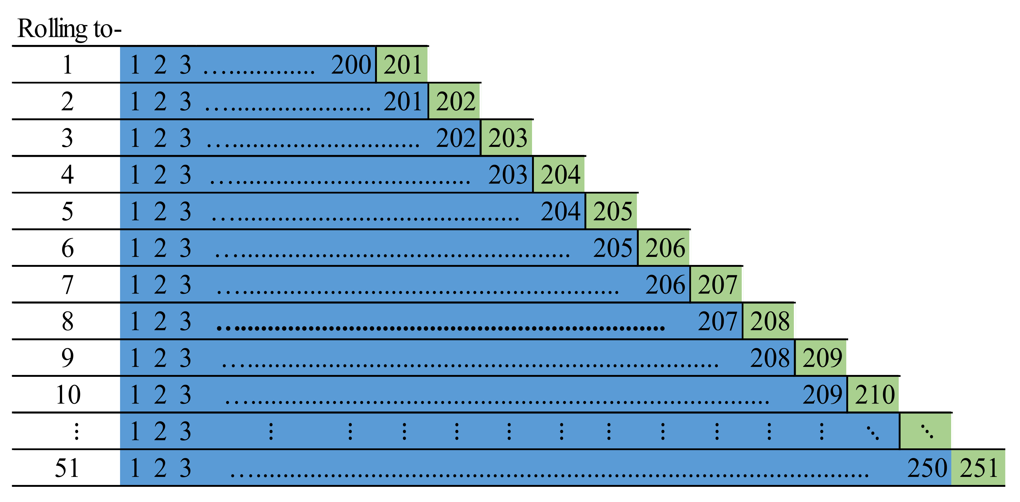
- Splitting data according to the rolling origin cross-validation (ROCV) series
- 2.
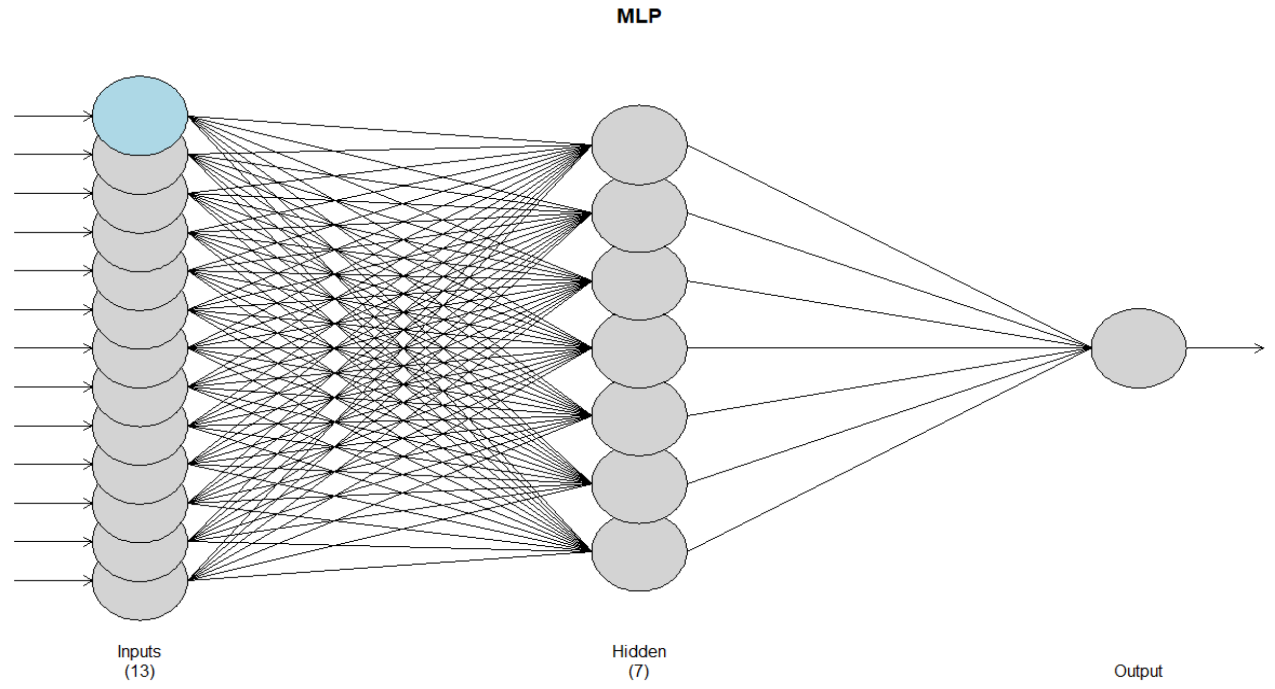
- Structure of the network architecture
- 3.
- Selection of the activation function
- 4.
- Normalization of data
- 5.
- Implementation of training and testing processes
- 6.
- Evaluation of the forecast model from the MAPE value
- 7.
- Prediction of exogenous variables
- 8.
- Prediction of main variables
3. Results
3.1. NARX NN Model Formation
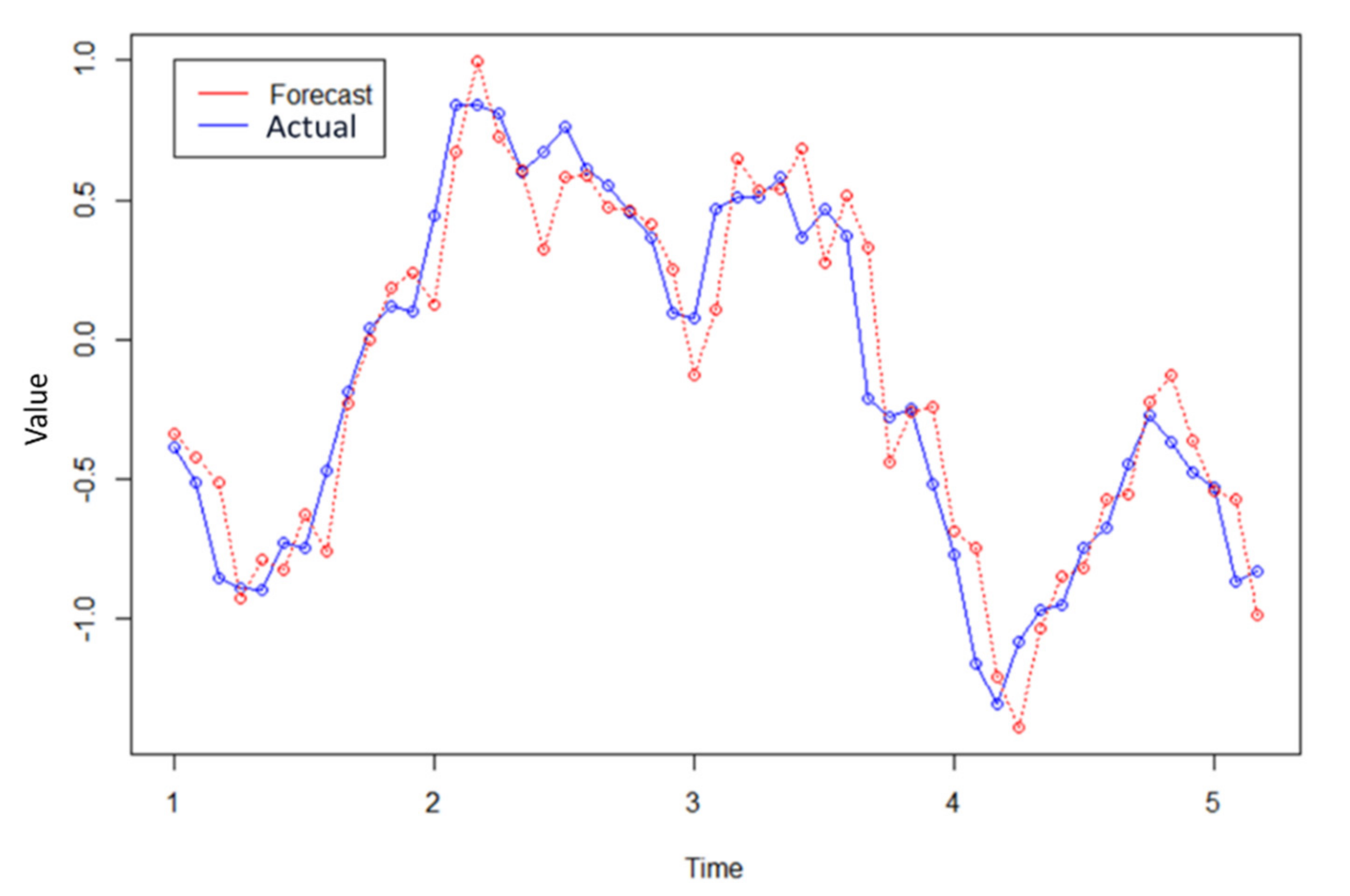
3.2. Forecasting Exogenous Variables (Niño 3.4)
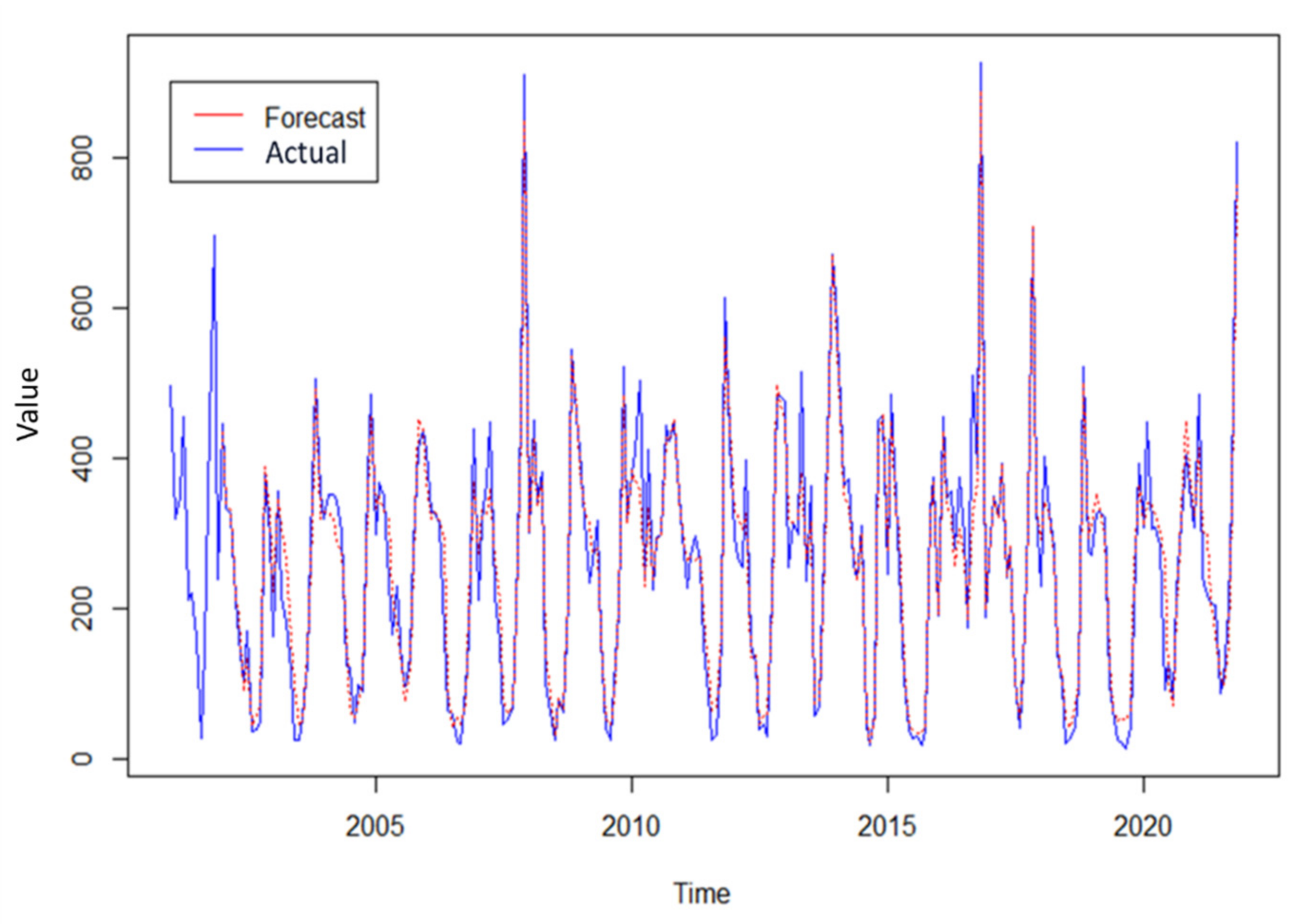
3.3. Forecasting the Main Variable (Rainfall)
4. Discussion
5. Conclusions
Author Contributions
Funding
Institutional Review Board Statement
Informed Consent Statement
Data Availability Statement
Conflicts of Interest
References
- Utina, R. Global Warming. Jurnal SAINTEK UNG. 2009, pp. 1–11. Available online: https://repository.ung.ac.id/karyailmiah/show/324/pemanasan-global-dampak-dan-upaya-meminimalisasinya.html (accessed on 2 February 2022).
- Iyakaremye, V.; Zeng, G.; Yang, X.; Zhang, G.; Ullah, I.; Gahigi, A. Science of the Total Environment Increased high-temperature extremes and associated population exposure in Africa by the mid-21st century. Sci. Total Environ. 2021, 790, 148162. [Google Scholar] [CrossRef] [PubMed]
- Mulyani, A.S. Global Warming, Causes, Impacts and Anticipation. 2021. Available online: http://repository.uki.ac.id/4908/1/PEMANASANGLOBAL.pdf (accessed on 2 February 2022).
- Iyakaremye, V.; Zeng, G.; Ullah, I.; Gahigi, A.; Mumo, R.; Ayugi, B. Recent Observed Changes in Extreme High-Temperature Events and Associated Meteorological Conditions over Africa. Int. J. Climatol. 2021. [Google Scholar] [CrossRef]
- Sipayung, S. The Spectrum Analysis of Meteorogical Elements in Indonesia. Master’s Thesis, Nagoya University, Nagoya, Japan, 1995. [Google Scholar]
- Pramudia, A. Climate Dynamics in Indonesia; Agricultural Research and Development Agency: Jakarta, Indonesia, 2020. [Google Scholar]
- McBride, M.; Haylock, M.R.; Nicholls, N. Relationships between the Maritime Continent Heat Source and the El Niño–Southern Oscillation Phenomenon Relationships between the Maritime Continent Heat Source and the El Niño–Southern Oscillation Phenomenon. J. Clim. 2003, 0442, 2905–2914. [Google Scholar] [CrossRef] [Green Version]
- Sein, Z.M.M.; Ullah, I.; Iyakaremye, V.; Azam, K.; Ma, X.; Syed, S.; Zhi, X. Observed spatiotemporal changes in air temperature, dew point temperature and relative humidity over Myanmar during 2001–2019. Meteorol. Atmos. Phys. 2022, 134, 10–15. [Google Scholar] [CrossRef]
- Sein, Z.M.M.; Zhi, X.; Ullah, I.; Azam, K.; Ngoma, H.; Saleem, F.; Xing, Y.; Iyakaremye, V.; Syed, S.; Hina, S.; et al. Recent variability of sub-seasonal monsoon precipitation and its potential drivers in Myanmar using in-situ observation during 1981–2020. Int. J. Climatol. 2021. [Google Scholar] [CrossRef]
- Robinson, P.J.; Henderson-Sellers, A. Contemporary Climatology; Routledge: New York, NY, USA, 2014. [Google Scholar]
- Tjasyono, B. Meteorologi Indonesia; Meteorology Climatology and Geophysics Council Meteorology, Climatology and Geophysics Agency: Jakarta, Indonesia, 2012; Volume 1. [Google Scholar]
- IPRC. International Pasific Research Center. IPRC Climate. 2012. Available online: http://iprc.soest.hawaii.edu/ (accessed on 2 February 2022).
- Ina, J.; Ruminta Bayong, T.H.; Atika, L.; Harijono, S.B. The Effect of El Niño, La Niña and Indian Ocean Dipole on Pentad Rainfall in Indonesia. J. Bionatura 2008, 10, 168–177. Available online: https://www.google.com/url?sa=t&rct=j&q=&esrc=s&source=web&cd=&ved=2ahUKEwjVx92QlfX1AhU3iv0HHZsQBgkQFnoECAwQAQ&url=https%3A%2F%2Fjurnal.unpad.ac.id%2Fbionatura%2Farticle%2Fdownload%2F7735%2F3591&usg=AOvVaw1eWTNIOGVSUyHyXFO-HL1t (accessed on 13 January 2022).
- Rudiyanto, A. Atmospheric Climate Projection, Bappenas, Jakarta, Indonesia. 2018. Available online: https://lcdi-indonesia.id/wp-content/uploads/2020/05/Proyeksi-Iklim-Atmosferik (accessed on 2 February 2022).
- Anisa, K.N. Analysis of the Relationship between Rainfall and El-Nino Southern Oscillation Indicators in East Java Rice Production Centers Using the Copula Approach. J. Sains Seni 2015, 4, 146. [Google Scholar]
- Oded, M. Government Agencies Performance, PPIDBandung, Bandung, Indonesia. 2020. Available online: https://ppid.bandung.go.id/wp-content/uploads/2021/07/LKIP-Kota-Bandung-2020 (accessed on 2 February 2022).
- Jabar. Prov, Bandung City Profile. PPIDBandung, Bandung, Indonesia. 2020. Available online: https://ppid.bandung.go.id/?media_dl=9872 (accessed on 2 February 2022).
- Gutomo, M.d.T. Flood and Landslide Natural Disasters and Community Efforts in Mitigating. J. PKS 2015, 14, 437–452. [Google Scholar]
- Tempo.co. Hegarmanah, Bandung Hit by Flood. 2008. Available online: https://nasional.tempo.co/read/116481/hegarmanah-bandung-diterjang-banjir (accessed on 2 February 2022).
- Putra, M.A. A Total of 16 Points in Bandung Were Submerged by Floods. 2016. Available online: https://www.cnnindonesia.com/nasional/20161114000828-20-172377/sebanyak-16-titik-di-bandung-terendam-banjir (accessed on 2 February 2022).
- Kartika, T.; Sulandari, W.; Pratiwi, H. Forecasting rainfall in the city of Bandung using singular spectrum analysis. J. Ilm. Mat. 2021, 8, 56–65. [Google Scholar]
- Danung, A. Floods Inundate Six Districts in Bandung Regency. 2020. Available online: https://bnpb.go.id/berita/banjir-rendam-enam-kecamatan-di-kabupaten-bandung (accessed on 2 February 2022).
- UCSB CHIRPS v2p0 Monthly Global CHIRPS Precipitation. 2021. Available online: https://iridl.ldeo.columbia.edu/SOURCES/.UCSB/.CHIRPS/.v2p0/.monthly/.global/.precipitation/X/%28110.85E%29VALUES/T/%28Jan2021%29%28Sep2021%29RANGEEDGES/Y/%287.075S%29VALUES/datatables.html (accessed on 13 January 2022).
- APCC. Pacific SST Indices Monitoring. 2021. Available online: https://apcc21.org/ser/indic.do?lang=en (accessed on 13 January 2022).
- Desouky, M.A.A.; Abdelkhalik, O. Wave prediction using wave rider position measurements and NARX network in wave energy conversion. Appl. Ocean Res. 2019, 82, 10–21. [Google Scholar] [CrossRef]
- Zhang, G.; Patuwo, B.E.; Hu, M.Y. Forecasting with artificial neural networks: The state of the art. Int. J. Forecast. 1998, 14, 35–62. [Google Scholar] [CrossRef]
- Ghamariadyan, M.; Imteaz, M.A. A wavelet artificial neural network method for medium-term rainfall prediction in Queensland (Australia) and the comparisons with conventional methods. Int. J. Climatol. 2021, 41, E1396–E1416. [Google Scholar] [CrossRef]
- Shrivastava, G. Application of Artificial Neural Networks in Weather Forecasting: A Application of Artificial Neural Networks in Weather Forecasting: A Comprehensive Literature Review. Int. J. Comput. Appl. 2012, 51, 17–29. [Google Scholar] [CrossRef]
- Pham, B.T.; Le, L.M.; Le, T.-T.; Bui, K.-T.T.; Le, V.M.; Ly, H.-B.; Prakash, I. Development of advanced artificial intelligence models for daily rainfall prediction. Atmos. Res. 2020, 237, 104845. [Google Scholar] [CrossRef]
- Diez-Sierra, J.; Jesus, M. Long-term rainfall prediction using atmospheric synoptic patterns in semi- arid climates with statistical and machine learning methods. J. Hydrol. 2020, 586, 124789. [Google Scholar] [CrossRef]
- Rahman, S.; Reza, A. Are precipitation concentration and intensity changing in Bangladesh overtimes? Analysis of the possible causes of changes in precipitation systems. Sci. Total Environ. 2019, 690, 370–387. [Google Scholar] [CrossRef]
- Ruiz, L.G.B.; Cuéllar, M.P.; Calvo-Flores, M.D.; Jiménez, M.D.C.P. An Application of Non-Linear Autoregressive Neural Networks to Predict Energy Consumption in Public Buildings. Energies 2016, 9, 684. [Google Scholar] [CrossRef] [Green Version]
- Ranjit, K.P.; Sinha, K. Forecasting crop yield: A comparative assessment of arimax and narx model. Indian Agric. Stat. Res. Inst. 2016, 1, 77–85. [Google Scholar]
- Wunsch, A.; Liesch, T.; Broda, S. Forecasting groundwater levels using nonlinear autoregressive networks with exogenous input (NARX). J. Hydrol. 2018, 567, 743–758. [Google Scholar] [CrossRef]
- Boussaada, Z.C. A Nonlinear Autoregressive Exogenous (NARX) Neural Network Model for the Prediction of the Daily Direct Solar Radiation. Energies 2018, 11, 620. [Google Scholar] [CrossRef] [Green Version]
- Fausett, L. Fundamentals of Neural Networks Architectures, Algorithms, and Applications; Prentice Hall, Inc.: London, UK, 1994. [Google Scholar]
- Cadenas, E.; Rivera, W.; Campos-Amezcua, R.; Heard, C. Wind Speed Prediction Using a Univariate ARIMA Model and a Multivariate NARX Model. Energies 2016, 9, 109. [Google Scholar] [CrossRef] [Green Version]
- Chen, R.J.; Bloomfield, P.; Fu, J.S. An evaluation of alternative forecasting methods to recreation visitation. J. Leis. Res. 2003, 35, 441–454. [Google Scholar] [CrossRef]
- Gao, Y.; Er, M.J. NARMAX time series model prediction: Feedforward and recurrent fuzzy neural network approaches. Fuzzy Sets Syst. 2014, 150, 331–350. [Google Scholar] [CrossRef]
- Hyndman, R.J.; Athanasopoulos, G. Forecasting: Principles and Practice; Monash University: Melbourne, Australia, 2018. [Google Scholar]
- Rianto, Y.; Kuntoro, A.Y. Prediction of Netizen Tweets Using Random Forest, Decision Tree, Naïve Bayes, and Ensemble Algorithm. Sinkron 2020, 5, 58–71. [Google Scholar]
- Ladiray, D.; Palate, J.; Mazzi, G.; Proietti, T. Seasonal Adjustment of Daily Data. In Proceedings of the 16th Conference of IAOS, Paris, France, 19–21 September 2018; pp. 1–26. [Google Scholar]
- Feng, J.; Lu, S. Performance Analysis of Various Activation Functions in Artificial Neural Networks. J. Phys. 2019, 1237, 022030. [Google Scholar] [CrossRef]
- Anastasiadis, A.D.; Magoulas, G.D.; Vrahatis, M.N. An Efficient Improvement of the Rprop Algorithm. In Artificial Neural Networks in Pattern Recognition (ANNPR 2003), Proceedings of the First International Association of Pattern Recognition-TC3 Workshop (IAPR 2003), Florence, Italy, 12–13 September 2003; Gori, M., Marinai, S., Eds.; Springer: Berlin/Heidelberg, Germany, 2003; pp. 197–201. [Google Scholar]
- Ghoshal, B.; Tucker, A.; Sanghera, B.; Wong, W.L. Estimating uncertainty in deep learning for reporting confidence to clinicians in medical image segmentation and diseases detection. Comput. Intell. 2019, 37, 701–734. [Google Scholar] [CrossRef]
- Ullah, I.; Ma, X.; Yin, J.; Saleem, F.; Syed, S.; Omer, A.; Habtemicheal, B.A.; Liu, M.; Arshad, M. Observed changes in seasonal drought characteristics and their possible potential drivers over Pakistan. Int. J. Climatol. 2021. [Google Scholar] [CrossRef]
- Shahzaman, M.; Zhu, W.; Ullah, I.; Mustafa, F.; Bilal, M.; Ishfaq, S.; Nisar, S.; Arshad, M.; Iqbal, R.; Aslam, R.W. Comparison of multi-year reanalysis, models, and satellite remote sensing products for agricultural drought monitoring over south asian countries. Remote Sens. 2021, 13, 3294. [Google Scholar] [CrossRef]
- Shahzaman, M.; Zhu, W.; Bilal, M.; Habtemicheal, B.A.; Mustafa, F.; Arshad, M.; Ullah, I.; Ishfaq, S.; Iqbal, R. Remote sensing indices for spatial monitoring of agricultural drought in south asian countries. Remote Sens. 2021, 13, 2059. [Google Scholar] [CrossRef]
- Hina, S.; Saleem, F.; Arshad, A.; Hina, A.; Ullah, I. Droughts over Pakistan: Possible cycles, precursors and associated mechanisms. Geomat. Nat. Hazards Risk 2021, 12, 1638–1668. [Google Scholar] [CrossRef]
- Sein, Z.M.M.; Ullah, I.; Syed, S.; Zhi, X.; Azam, K.; Rasool, G. Interannual variability of air temperature over myanmar: The influence of enso and iod. Climate 2021, 9, 35. [Google Scholar] [CrossRef]
- Sein, Z.M.M.; Ullah, I.; Saleem, F.; Zhi, X.; Syed, S.; Azam, K. Interdecadal variability in myanmar rainfall in the monsoon season (May–october) using eigen methods. Water 2021, 13, 729. [Google Scholar] [CrossRef]
- Jati, R. Susur Sungai Upaya Cegah Potensi Bahaya Banjir Bandang. BNPB. 2020. Available online: https://bnpb.go.id/berita/susur-sungai-upaya-cegah-potensi-bahaya-banjir-bandang- (accessed on 2 February 2022).
- Toharudin, T.; Pontoh, R.S.; Caraka, R.E.; Zahroh, S.; Lee, Y.; Chen, R.C. Employing long short-term memory and Facebook prophet model in air temperature forecasting. Commun. Stat.-Simul. Comput. 2021. [Google Scholar] [CrossRef]


| Unit | Specifications |
|---|---|
| Input unit | 13 units, consisting of lag 1, 2, …, 365 from rainfall and the current value of Niño 3.4 index |
| Hidden layer | 1 layer |
| Hidden unit | 1, 2, 3, 4, 5, 6, 7 unit (trial and error) |
| Output unit | 1 unit |
| Architecture | Hidden Unit | MAPE Test |
|---|---|---|
| Input unit = 13 Hidden layer = 1 | 1 | 6.399138 |
| 2 | 6.935423 | |
| 3 | 6.613024 | |
| 4 | 6.587894 | |
| 5 | 6.809819 | |
| 6 | 6.857698 | |
| 7 | 6.259928 |
| Unit | Specifications |
|---|---|
| Input unit | 12 unit (lag 1, 2, …, 12) |
| Hidden layer | 1 layer |
| Hidden unit | 1, 2, 3, 4, 5, 6, 7 unit (trial and error) |
| Output unit | 1 unit |
| Architecture | Hidden Unit | MAPE Test |
|---|---|---|
| Input unit = 12 Hidden layer = 1 | 1 | 4.53155 |
| 2 | 4.501856 | |
| 3 | 4.514769 | |
| 4 | 4.500933 | |
| 5 | 4.443294 | |
| 6 | 4.623074 | |
| 7 | 7.566102 |
| Period | Forecast |
|---|---|
| December 2021 | −0.6212955 |
| January 2022 | −0.6976738 |
| February 2022 | −0.5343275 |
| March 2022 | −0.4814957 |
| April 2022 | −0.3752520 |
| May 2022 | −0.2630829 |
| Period | Forecast |
|---|---|
| December 2021 | 277.7361 |
| January 2022 | 273.1235 |
| February 2022 | 342.9711 |
| March 2022 | 335.8127 |
| April 2022 | 276.0515 |
| May 2022 | 170.4804 |
Publisher’s Note: MDPI stays neutral with regard to jurisdictional claims in published maps and institutional affiliations. |
© 2022 by the authors. Licensee MDPI, Basel, Switzerland. This article is an open access article distributed under the terms and conditions of the Creative Commons Attribution (CC BY) license (https://creativecommons.org/licenses/by/4.0/).
Share and Cite
Pontoh, R.S.; Toharudin, T.; Ruchjana, B.N.; Sijabat, N.; Puspita, M.D. Bandung Rainfall Forecast and Its Relationship with Niño 3.4 Using Nonlinear Autoregressive Exogenous Neural Network. Atmosphere 2022, 13, 302. https://doi.org/10.3390/atmos13020302
Pontoh RS, Toharudin T, Ruchjana BN, Sijabat N, Puspita MD. Bandung Rainfall Forecast and Its Relationship with Niño 3.4 Using Nonlinear Autoregressive Exogenous Neural Network. Atmosphere. 2022; 13(2):302. https://doi.org/10.3390/atmos13020302
Chicago/Turabian StylePontoh, Resa Septiani, Toni Toharudin, Budi Nurani Ruchjana, Novika Sijabat, and Mentari Dara Puspita. 2022. "Bandung Rainfall Forecast and Its Relationship with Niño 3.4 Using Nonlinear Autoregressive Exogenous Neural Network" Atmosphere 13, no. 2: 302. https://doi.org/10.3390/atmos13020302
APA StylePontoh, R. S., Toharudin, T., Ruchjana, B. N., Sijabat, N., & Puspita, M. D. (2022). Bandung Rainfall Forecast and Its Relationship with Niño 3.4 Using Nonlinear Autoregressive Exogenous Neural Network. Atmosphere, 13(2), 302. https://doi.org/10.3390/atmos13020302