Abstract
Air-quality monitoring and analysis are initial parts of a comprehensive strategy to prevent air pollution in cities. In such a context, statistical tools play an important role in determining the time-series trends, locating areas with high pollutant concentrations, and building predictive models. In this work, we analyzed the spatio-temporal behavior of the pollutant PM10 in the Monterrey Metropolitan Area (MMA), Mexico during the period 2010–2018 by applying statistical analysis to the time series of seven environmental stations. First, we used experimental variograms and scientific visualization to determine the general trends and variability in time. Then, fractal exponents (the Hurst rescaled range and Higuchi algorithm) were used to analyze the long-term dependence of the time series and characterize the study area by correlating that dependence with the geographical parameters of each environmental station. The results suggest a linear decrease in PM10 concentration, which showed an annual cyclicity. The autumn-winter period was the most polluted and the spring-summer period was the least. Furthermore, it was found that the highest average concentrations are located in the western and high-altitude zones of the MMA, and that average concentration is related in a quadratic way to the Hurst and Higuchi exponents, which in turn are related to some geographic parameters. Therefore, in addition to the results for the MMA, the present paper shows three practical statistical methods for analyzing the spatio-temporal behavior of air quality.
1. Introduction
Since ancient times, the behavior of the different variables that interact in the atmosphere has drawn the attention of human beings, as these variables set the guidelines for the conditions of the environment in which daily activities are carried out. The study of pollutant behavior has become an important and relevant topic in a society that aspires to improve quality of life.
Air pollution is defined as the presence of one or more chemical substances in the air at high concentrations that can damage human beings, animals, vegetation, and even materials [1,2,3,4]. Some of the pollutants studied and measured are ozone (O3), sulfur dioxide (SO2), nitrogen dioxide (NO2), carbon monoxide (CO), lead (Pb), and particulate matter (PM). The Norma Oficial Mexicana NOM-025-SSA1-2014 [5] describes PM as a mix of substances in a solid or liquid state that remains suspended in the atmosphere. Each particle can present a wide variety of features. Therefore, to better study it, this material is classified into two groups according to its aerodynamic behavior— PM2.5 and PM10, which are less than 2.5 μm and 10 μm, respectively [4,6,7,8].
One way to examine the impact of pollutants on the environment is through their time series. Different methodologies have been used to study this, such as that of Arreola Contreras and González [9], in which a spectral analysis is applied to time series, with which they found that wind is correlated with the tracking of PM10 levels. Likewise, Lee et al. [10] indicate that it is possible to use Box counting as a tool to distinguish spatio-temporal variations of PM10.
As a temporal population variance estimator and structural analysis model, a variogram describes the relation of paired observations separated by a distance h. Specifically, this method consists of estimating the expected value of the squared difference between neighboring random variables separated by different values of h throughout the time series, providing fundamental support and allowing the representation of such a relation quantitatively, as well as determining important aspects of the series such as the distance at which the maximum variability occurs, whether there is cyclicity or not, and whether to perform interpolation or kriging [11,12]. Several authors have studied the temporal variation of PM10, correlating its variability with other variables such as wind direction, temperature, and diurnal cycle, among others [13,14,15,16,17,18]. In turn, Serna [19] explains how a variogram can have different applications, such as when there is uncertainty if a time series can be stationary or non-stationary.
On the other hand, fractal exponents, such as the Hurst rescaled range [20] and the Higuchi fractal dimension [21], measure the fractality of time series, which is directly related to the persistency or long-term memory of time series. Therefore, the higher the value in the exponent, the higher the persistence. Several analyses relating the dependence of long-term memory on different pollutants have been reported in the literature [22,23,24,25,26]. was used as the primary tool in those reports, which found a long-term correlation for PM10 results. Additionally, Nikolopoulos et al. [23] used the algorithm to study PM10 time series, indicating fractality and long-term memory in the behavior of the records from the studied stations. However, none of these exponents have been calculated to compare them with geographic parameters, such as latitude, longitude, and altitude, despite the fact that those relations have been found for other meteorological variables [27,28,29,30].
Regarding standards and other studies undertaken in Mexico, air pollution has been considered a serious and complex issue in this country since the 1970s, which has resulted in the design new techniques to study this phenomenon [31,32,33]. Among these researches, Audelo-Vucovich et al. [34] stand out, having used the Hurst exponent and other tools to determine the persistence of PM10 concentrations and their correlation with environmental pre-contingency, observing that the probability of reaching a pre-contingency event increases when .
Moving deeper into the study area, different strategies have been established in the Monterrey Metropolitan Area (MMA), given the city’s characteristics and accelerated urban growth. In the mid-1990s, PM10 and O3 pollutants frequently registered values that exceeded the established level limit of the air quality standards [35]. In this context, the government of the State of Nuevo León, in the Environmental State Plan 1995–2020 (Plan Estatal de Medio Ambiente 1995–2020), defined guidelines and developed the Administration of Air Quality Program 1997–2000 (Programa de Administración de la Calidad del Aire del AMM 1997–2000) [36]. As a result, the region uses an environmental monitoring system called the Sistema Integral de Monitoreo Ambiental (SIMA), which keeps track of air quality based on the criteria pollutants (CO, SO2, , O3, PM10, and PM2.5). Recently, air pollution was analyzed between 2006 and 2008, comparing PM10 levels at different time scales (seasons and days) and employing the Bootstrap method to obtain samples studied under a variance analysis [37]. It was found that PM10 values were high and exceeded the 75 μg/m3 per day limit determined by NOM-025-SSA1-2014 in 2014 [5], and it was concluded that these levels may have severe effects on health. The southern MMA had higher PM10 levels during the studied period. Winter was the most polluted season and summer the least. The most polluted days were Thursday and Friday, while Sunday was the least. The hours with the highest PM10 levels were from 8:00 to 10:00 a.m., while the hours during the night had the lowest levels. Moreover, according to SIMA records, the state government has issued continuous pollution alerts in recent years, meaning that there were more than 200 days per year of poor-quality air reported by at least one environmental station in the MMA [38]. In addition, a connection has been reported between chronic exposure to particle pollution and lead in blood, as well as uncommon common diseases [39] such as cleft lip and palate [40]. Similar studies outside the region have found a clear correlation between pollutants and obesity [41,42,43].
In this work, we carried out a spatio-temporal analysis of PM10 pollution in the MMA for the period 2010–2018 with two main objectives, the first being to provide a current and detailed quantification of temporary and geographic pollutant behavior to help to visualize the trend and distribution of pollution in the MMA, focusing on the periodicity of the time series and the detection of the most polluted zones inside the study area. For this purpose, we analyzed time series, variograms, and averaged data. The second objective was to determine the feasibility of using fractal coefficients, such as and , to provide outstanding information for PM10 time series analysis, taking into account the relations reported between those coefficients, geographic parameters, and other accumulated meteorological variables. The structure of the paper is as follows. The methodology used to construct the experimental variograms and calculate and is shown in Section 2; results and their interpretation are discussed in Section 3 and Section 4, respectively. Finally, conclusions are shown in Section 5.
2. Methodology
2.1. Data Acquisition and General Observations
Data were obtained from the monthly reports published by the government of Nuevo León throughout SIMA [44] meaning that the data were validated and published as open access. SIMA used a gravimetric method based on the Reference Method for the Determination of Suspended Particulate Matter in the Atmosphere (High-Volume Method) [45], which is also the official method established by the federal code regulations of the USA [46]. The minimum period interval used in the SIMA reports is one month. We used this minimum time length to obtain the maximum amount data for our analysis for the following reasons. First, despite the fact that nowadays there are 14 working environmental stations, we collected only the information of the seven stations with more records, since the other seven stations have significant missing data or have started to work only recently. The location of the selected environmental stations and the map of the MMA are illustrated in Figure 1. The time series used are from January 2010 to December 2018. This period was chosen because additional changes regarding the distribution of data reports were made starting in June 2019. Therefore, no treatment was performed on the database; all the information analyzed is raw data. Each time series comprises about 108 data points, corresponding to 9 years of information.
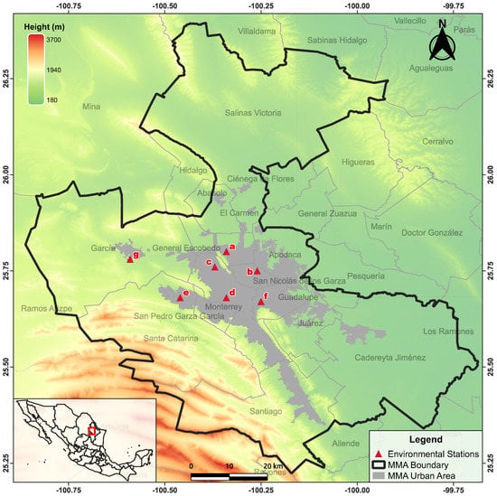
Figure 1.
SIMA environmental stations selected for this study: (a) North Station, (b) Northeast Station, (c) Northwest Station, (d) Center Station, (e) Southwest Station, (f) Southeast Station, (g) Northwest2 Station.
In Section 2.2–Section 2.4, we used the experimental semi-variogram and Hrs and HFD exponents to analyze these series. Additionally, we compared those data with some air quality standards to estimate how high the pollution level is in relation to health risk. The national standard that we used is NOM-025-SSA1-2014 [5], while the international standard considered is that proposed by the WHO for the year 2021 [47]. The classification intervals for air quality of both standards are shown in Table 1.

Table 1.
Labels used to define the air quality and health risk according to [5,47,48]. The last column corresponds to the corresponding PM10 intervals.
2.2. Experimental Semi-Variogram
Let a time series of PM10 concentration be . The semi-variogram of such a series is the half variance of the difference between pairs of observations separated by temporal distances h, such that [49,50]:
We used the discretized version of the estimator shown in Equation (1) to complete the semi-variograms of our PM10 series:
where refers to the number of temporal distances with a length h (in months) for the time series .
2.3. Hurst Exponent
The Hurst rescaled range () was measured for each time series X. The procedure consists of dividing X into d subseries [51,52]. Then, the respective rescaled range is obtained by:
where is the mean of the subseries , and represents the cumulative series of deviations considering values until the j-th subseries.
Next, the range shown in Equation (3) is rescaled and averaged, such that:
where is the standard deviation of the series .
Finally, is the exponent H that satisfies the power law:
where is a dimensionless constant. Practically, is calculated by applying the logarithm function to both sides of Equation (5), obtaining
The transformation of Equation (6) allows obtaining the coefficient H by a linear fitting of the points, using the Least Squares Method (). A key point in determining is the number of subseries m in which the temporal series is divided. In this work, we take because of the annual periodicity of the data.
2.4. Higuchi Fractal Dimension (HFD)
The Higuchi fractal dimension (HFD) was calculated according to Higuchi [21]. Similar to , divides the total time series into windows; however, its methodology is different since it does not calculate the range for the accumulative series, but for each subseries in a particular way. Namely, for a time series X with N data points [53],
expresses the fractal length of the subseries , where indicates the k-th time, m is the interval time of that subseries, and is the total number of subseries used. Therefore, the mean of all the ’s subseries (Equation (7)) defines the fractal length of the wide series, so that:
Similar to Hurst’s procedure, in practice, can be characterized by the slope F that fits the straight line equation:
which is obtained applying the corresponding logarithmic transformation from Equation (8). In Equation (9), is a constant, and F is a dimensionless constant. The fitting is performed by the . We used a maximum number of subseries in this work, considering the cyclical analysis for Hurst’s procedure and a good resolution in values.
3. Results
Figure 2 shows the time series of the monthly-averaged PM10 values for the environmental monitoring stations in the study area. In each graph, the time series corresponding to the parenthetical remarks (a) to (f), is compared with the time series corresponding to the Northwest2 station, because this environmental station differs from the others in some aspects. Namely, it recorded the highest PM10 levels during the study period despite the fact that the municipality is a sub-urban zone outside the MMA; see Figure 1. The majority of the stone quarries are located in this zone [54], there is a difference of 200 m between that municipality and the rest of the MMA, and the main wind direction is east-west, driving the particles of all the metropolitan area to this zone [9]. The semiannual averages are marked with a discontinuous horizontal line of the same color as the graph in the corresponding period. Background colors indicate the division of the years in six-month periods. Finally, the established thresholds are marked to classify air quality by Mexican norms NOM-025-SSA1-1993 and NOM-025-SSA1-2014 [5,48] by horizontal red lines; see Table 1 for the meaning of labels of air quality. The GL limit showed discontinuity in 2015, since there was a decrease in the classification criteria of the NOM-025-SSA1-2014, which took effect that year. The horizontal dashed line is the limit for good air quality established by the World Health Organization (WHO) [47].
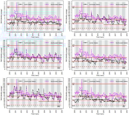
Figure 2.
Comparison of time series of monthly PM10 mean values between the Northwest2 Station and (a) North Station, (b) Northeast Station, (c) Northwest Station, (d) Center Station, and (e) Southwest Station, (f) Southeast Station. Air quality labels (red-horizontal lines) are described in Table 1. Vertical panels divide the window time into six-month periods to illustrate the periodicity of the series. Short-horizontal lines with a length of one year indicate the PM10 mean of that year for that time series.
Table 2 displays the results of the annual averages obtained from the time series and the Hrs and HFD exponents obtained from the procedures described in Section 2.3 and Section 2.4, respectively. In addition, the geographic information corresponding to each station is presented as well.
Table 2.
Hurst and Higuchi exponents, geographic parameters, PM10 mean, and air quality label of environmental stations in the MMA. The PM10 mean value corresponds to the entire studied period (2010–2018). The air quality label refers to the label corresponding to the PM10 mean value: AM = acceptable air quality and moderate health risk, PH = poor air quality and high health risk.
The pollution variance is calculated by the semi-variogram formula (2) and shown in Figure 3 for each station. In each graph, the variogram of the Northwest2 station is compared to those of the other stations. In addition, a linear fit indicating the general tendency (smoothing the oscillating phenomenon) of each station is displayed.
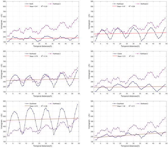
Figure 3.
Comparison of the semi-variogram of the Northwest2 Station with the other six stations. The red line is the data fitting.
4. Discussion
4.1. Time Series and Semi-Variograms
The results shown in the time series in Figure 2 indicate a general decrease in the last ten years. The variability analysis shown in Figure 3 allows us to quantify this tendency for each station.
Specifically, the Northwest2 station showed a more significant decrease than the others with a slope of 4.04 in contrast to slopes smaller than 1 for the other stations (Southeast has 1.82); see Figure 3. However, despite that decrease, the aforementioned station showed one of the highest pollution levels per six-month period, as is observable in the horizontal bars of the series shown in Figure 2. In turn, the stations located to the north and the west zones of the MMA showed a greater amount of pollution than the stations in the east. As previously reported [9], these observations indicate the accumulation of pollution in the western region caused by the predominant airflow in the east-to-west direction. This is essential knowledge for MMA inhabitants and authorities to identify or map the most dangerous zones inside the metropolis.
The time series of all the environmental stations exhibited an annual quasi-periodicity, which is clearly shown in most of the charts in Figure 3, except for the northern and southeastern stations. This phenomenon had already been suggested by González-Santiago et al. [37], who reported greater PM10 concentrations in winter and minor concentrations in summer during 2006–2008. We found that this periodic tendency remained for 2010–2018. Indeed, aided by the division of background colors in the charts of Figure 2, greater PM10 concentrations can be observed in the autumn-winter period than in the spring-summer period for all of the MMA. This suggests that the quasi-periodic behavior of the time series is a natural phenomenon of the region that could be related to other environmental factors that have been reported with the same cyclical characteristics for the study area, such as the seasonal rains of the region [55].
The decrease of PM10 concentrations over time could also be a natural phenomenon or it could be caused by the actions of the corresponding government, since the federal government establishes the air quality reference limits while the state government is in charge of establishing measures to fulfill these limits. As is observable in the charts of Figure 2, although there are some stations in the interval of PH, and in particular cases, with historical records reaching VV, the values tended to decrease as previously mentioned, and managed to balance within the AM-GL ranges in the case of the North, Center, and Southeast stations. When analyzing the different periods of the seasons of the year, it can be observed that the highest peaks of all time series are concentrated in the period from autumn-winter 2010 to the beginning of spring-summer 2011. Authorities have associated those high PM10 concentrations to three atmospheric factors [56]. The first is the lack abundance of rainfall from October 2010, which brought droughts. The second one is the low relative humidity index due to a significant increase in temperature. The third is related to the speed and direction of winds, since strong winds with speeds of 20 to 40 km/h and an average flow in the east-west direction in the MMA caused all the particulate matter that was part of the ground to enter atmospheric suspension once again and consequently increase the PM10 indices.
Additionally, it can also be observed that time series of the Northwest, Northwest2, and Southwest stations oscillate around the AM limit with their PM10 mean value in the PH interval; see Table 1. The other stations oscillate between lower values compared to the previous ones, from GL to AM.
4.2. Fractal Exponents, PM10 Mean, and Geographic Parameters
According to the obtained results, it is possible to classify the seven time series as a correlation or long-term memory due to the Hurst and Higuchi exponents, with and values for all the stations.
We found that the geographic parameters are as much related to the fractal exponents that were used as to the average PM10 concentration. In detail, the average value of PM10 follows has a quadratic behavior related to increase in altitude; i.e., the greater the height, the greater the PM10 concentration; see Figure 4. This relation has a fitting of , whereas and do not have a clear relation, as they obtained low values in their quadratic fitting: 0.23 and 0.01, respectively.
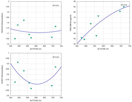
Figure 4.
Relation between altitude and , PM10 mean, and , respectively. Blue lines represent data fitting and R2 is the coefficient of determination.
The fittings of , , and the PM10 mean for the longitude of the stations have a behavior similar to that of altitude. As seen in Figure 5, the curve of Hurst, as well as that of Higuchi, has a concave-upwards-quadratic behavior, with bad fitting , whereas the curve of PM10 mean is concave downwards and presents very good fitting (); in fact, the pollution concentration grows in the stations located mainly in the western zone.
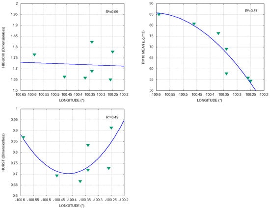
Figure 5.
Relation between longitude and , PM10 mean, and , respectively. Blue lines represent data fitting and R2 is the coefficient of determination.
This last observation and the PM10-altitude relation were expected due to the predominant airflow and the suspension of such particles in the air, as commented on in Section 4.1. In response to these clear tendencies, it can be concluded that the population of the west zone of the MMA is more susceptible to suffering diseases (e.g., cleft lip and palate [40]) caused by PM10 than the people living in the central and eastern zones. This encourages the development of initiatives in which the government can take preventive action, either segmented or clustered within the MMA, focusing on its western zone.
On the other hand, Figure 6 shows that latitude is mainly related to the values obtained from the in a quadratic way (), whereas fits with ; the quadratic curves fitted by both methods reach their minimum value in latitude between 25.70° and 25.75°. Moreover, the PM10 mean does not have a clear relation with latitude (). Even though the series are persistent according to , we cannot clearly explain the good fit between the long-term correlation measured by and the latitude. In addition, there is good quadratic fitting for the Higuchi-PM10 mean () and Hurst-PM10 mean () (see Figure 7), which we think should be studied in more detail by increasing the number of environmental monitoring stations in future work, since this could help to numerically characterize the behavior of PM10 through the persistence of its time series and fractal exponents.
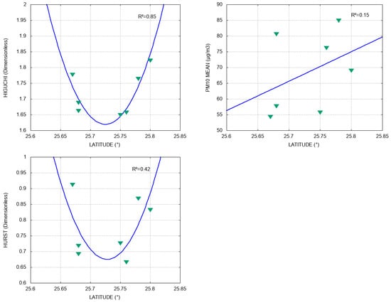
Figure 6.
Relation between latitude and , PM10 mean, and , respectively. Blue lines represent data fitting and R2 is the coefficient of determination.
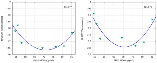
Figure 7.
Relation between PM10 mean and and , respectively. Blue lines represent data fitting and R2 is the coefficient of determination.
5. Conclusions
Seven time series of the air pollutant PM10 taken from environmental monitoring stations located in the Monterrey Metropolitan Area (MMA), Mexico, were analyzed, with the following results obtained:
- The annual cyclical behavior reported in previous studies was the same for the period studied, from 2010 to 2018, with greater pollution levels during the autumn-winter periods and lower levels during spring-summer periods;
- The PM10 concentration has been decreasing, which is promising for the people of the MMA in the near future. Nevertheless, half of the selected stations exceeded the AM limit during their most polluted period. Therefore, studying strategies to deal with pollution can help the authorities make decisions that protect the environment and the quality of life of MMA inhabitants;
- The highest values of average pollution are located in the western zone and the zone with the highest altitude in the MMA, which is probably a consequence of the main direction of wind flow, as well as geographical features. Consequently, we suggest a personalized alert system for the interior of the MMA so that the state government can issue policies and warn people from different areas of the metropolis according to the level of contamination presented by each zone;
- The persistence of the series, measured with and , is related in a quadratic way to the pollution mean. We did not find a correlation between these coefficients and altitude, but we found a strong correlation between and latitude, which is a significant result since latitude was not related to PM10 mean level;
- The use of the semi-variograms and fractal exponents and provided practical results in the time series analysis, which suggests that these techniques should continue to explored and that they should be complemented with other meteorological parameters for the corresponding authorities to take into account in their decision making.
Author Contributions
Conceptualization, M.A.A.-L., R.S.-V. and F.G.B.-B.; methodology, M.A.A.-L., M.A.R.-G., R.S.-V. and F.G.B.-B.; software, M.A.R.-G., F.G.B.-B. and Á.G.B.-R.; validation, M.A.A.-L., R.S.-V., L.E.G.-S. and F.G.B.-B.; formal analysis, M.A.A.-L., R.S.-V. and F.G.B.-B.; investigation, M.A.R.-G., R.S.-V., L.E.G.-S., F.G.B.-B. and O.W.-G.; resources, M.A.A.-L., M.A.R.-G., R.S.-V., L.E.G.-S. and O.W.-G.; data curation, M.A.R.-G., Á.G.B.-R. and F.G.B.-B.; writing—original draft preparation, M.A.A.-L., M.A.R.-G., L.E.G.-S. and F.G.B.-B.; writing—review and editing, M.A.A.-L., M.A.R.-G., L.E.G.-S., R.S.-V., F.G.B.-B., O.W.-G. and M.G.P.-A.; visualization, M.A.A.-L., M.A.R.-G., R.S.-V., L.E.G.-S., Á.G.B.-R., F.G.B.-B. and O.W.-G.; supervision, M.A.A.-L., R.S.-V. and F.G.B.-B.; project administration, M.A.A.-L. and F.G.B.-B. All authors have read and agreed to the published version of the manuscript.
Funding
This research was funded by the Tecnológico Nacional de México, project number 10689.21-P.
Institutional Review Board Statement
Not applicable.
Informed Consent Statement
Not applicable.
Data Availability Statement
Data can be directly obtained from the SIMA’s website [44].
Acknowledgments
We thank the Facultad de Ciencias de la Tierra, Universidad Autónoma de Nuevo León, for the extra financial support given for this project.
Conflicts of Interest
The authors declare no conflict of interest.
References
- Alonso, E.; Martínez, W.; Rubio, J.C.; Velasco, F.; Chávez, H.L.; Ávalos, M.; Lara, C.; Cervantes, E. Calidad del Aire en Cuatro Ciudades de Michoacán, México: Su Efecto sobre Materiales de Construcción. Rev. Constr. 2007, 6, 66–74. [Google Scholar]
- Chan, C.K.; Yao, X. Air pollution in mega cities in China. Atmos. Environ. 2008, 42, 1–42. [Google Scholar] [CrossRef]
- Elliott, S.J.; Cole, D.C.; Krueger, P.; Voorberg, N.; Wakefield, S. The Power of Perception: Health Risk Attributed to Air Pollution in an Urban Industrial Neighbourhood. Risk Anal. 1999, 19, 621–634. [Google Scholar] [CrossRef] [PubMed]
- United States National Air Pollution Control Administration. Air Quality Criteria for Particulate Matter: Summary and Conclusions. 1969. Available online: https://files.eric.ed.gov/fulltext/ED070647.pdf (accessed on 30 December 2021).
- Secretaría de Salud. Norma Oficial Mexicana NOM-025-SSA1-2014, Salud ambiental. Valores límite Permisibles para la Concentración de Partículas Suspendidas PM10 y PM2.5 en el aire Ambiente y Criterios para su Evaluación. 2014. Available online: http://siga.jalisco.gob.mx/aire/normas/NOM-025-SSA1-2014.pdf (accessed on 30 December 2021).
- Santurtún Zarrabeitia, A. Contaminación Atmosférica, Tipos de Tiempo y Procesos Respiratorios en Santander y Zaragoza. Ph.D. Thesis, Universidad de Cantabria, Cantabria, Spain, 2014. [Google Scholar]
- Elvira, D.; Espinoza, P.; Claudia, I.; Molina, E. Contaminación del aire exterior Cuenca—Ecuador, 2009–2013. Posibles efectos en la salud. Rev. Fac. Cienc. Méd. Univ. Cuenca 2014, 32, 6–17. [Google Scholar]
- World Health Organization; Occupational and Environmental Health Team. Guías de Calidad del aire de la OMS Relativas al Material Particulado, el Ozono, el Dióxido de Nitrógeno y el dióXido de Azufre: Actualización Mundial 2005. 2006. Available online: https://apps.who.int/iris/handle/10665/69478 (accessed on 30 December 2021).
- Arreola Contreras, J.L.; González, G. Análisis espectral del viento y de partículas menores de 10 micrómetros (PM10) en el área metropolitana de Monterrey, México. Rev. Int. Contam. Ambient. 1999, 15, 95–102. [Google Scholar]
- Lee, C.K.; Ho, D.S.; Yu, C.C.; Wang, C.C. Fractal analysis of temporal variation of air pollutant concentration by box counting. Environ. Model. Softw. 2003, 18, 243–251. [Google Scholar] [CrossRef]
- Witt, A.; Malamud, B.D. Quantification of Long-Range Persistence in Geophysical Time Series: Conventional and Benchmark-Based Improvement Techniques. Surv. Geophys. 2013, 34, 541–651. [Google Scholar] [CrossRef]
- Gutiérrez-López, A.; Ramirez, A.I.; Lebel, T.; Santillán, O.; Fuentes, C. El variograma y el correlograma, dos estimadores de la variabilidad de mediciones hidrológicas. Rev. Fac. Ing. Univ. Antioq. 2011, 59, 193–202. [Google Scholar]
- Martínez, J.C. Aplicación del Modelaje Geoespacial en Geomática para Estimar los Niveles de Partículas Suspendidas PM10 en la Cuenca Atmosférica del Valle de México. Master’s Thesis, Centro de Investigación en Ciencias de Información Geoespacial, A.C., Mexico City, Mexico, 2011. [Google Scholar]
- Paez, M.; Gamerman, D.; de oliveira, V. Interpolation performance of a spatio-temporal model with spatially varying coefficients: Application to PM10 concentrations in Rio de Janeiro. Environ. Ecol. Stat. 2005, 12, 169–193. [Google Scholar] [CrossRef]
- Graeler, B.; Gerharz, L.; Pebesma, E. Spatio-Temporal Analysis and Interpolation of PM 10 Measurements in Europe. 2013. Technical Report. Available online: https://www.eionet.europa.eu/etcs/etc-atni/products/etc-atni-reports/etcacm_2012_8_spatio-temp_pm10analyses (accessed on 3 February 2022).
- Park, N.W. Time-Series Mapping of PM10 Concentration Using Multi-Gaussian Space-Time Kriging: A Case Study in the Seoul Metropolitan Area, Korea. Adv. Meteorol. 2016, 2016, 9452080. [Google Scholar] [CrossRef]
- Cabrera, J.B. A Geostatistical Method for the Analysis and Prediction of Air Quality Time Series: Application to the Aburrá Valley Region. Master’s Thesis, Technische Universität München, Munich, Germany, 2016. [Google Scholar]
- Gallardo, A. Geostadística. Ecosistemas 2007, 15. Available online: https://www.revistaecosistemas.net/index.php/ecosistemas/article/view/161 (accessed on 3 February 2022).
- Serna, J.M. Modelos Estadístico-Espaciales de Contaminantes del Aire en el Área Metropolitana de Monterrey. Master’s Thesis, Universidad Autónoma de Nuevo León, San Nicolás de los Garza, Mexico, 2020. [Google Scholar]
- Mandelbrot, B.B.; Wallis, J.R. Some long-run properties of geophysical records. Water Resour. Res. 1969, 5, 321–340. [Google Scholar] [CrossRef]
- Higuchi, T. Approach to an irregular time series on the basis of the fractal theory. Phys. D Nonlinear Phenom. 1988, 31, 277–283. [Google Scholar] [CrossRef]
- Meraz, M.; Rodriguez, E.; Femat, R.; Echeverria, J.; Alvarez-Ramirez, J. Statistical persistence of air pollutants (O3,SO2,NO2 and PM10) in Mexico City. Phys. A Stat. Mech. Its Appl. 2015, 427, 202–217. [Google Scholar] [CrossRef]
- Nikolopoulos, D.; Moustris, K.; Petraki, E.; Koulougliotis, D.; Cantzos, D. Fractal and Long-Memory Traces in PM10 Time Series in Athens, Greece. Environments 2019, 6, 29. [Google Scholar] [CrossRef]
- Krampah, F.; Amegbey, N.; Ndur, S.; Ziggah, Y.Y.; Hopke, P.K. Fractal Analysis and Interpretation of Temporal Patterns of TSP and PM10 Mass Concentration over Tarkwa, Ghana. Earth Syst. Environ. 2021, 5, 635–654. [Google Scholar] [CrossRef]
- Windsor, H.; Toumi, R. Scaling and persistence of UK pollution. Atmos. Environ. 2001, 35, 4545–4556. [Google Scholar] [CrossRef]
- Wang, J.; Shao, W.; Kim, J. Multifractal detrended cross-correlation analysis between respiratory diseases and haze in South Korea. Chaos Solitons Fractals 2020, 135, 109781. [Google Scholar] [CrossRef]
- Rehman, S. Study of Saudi Arabian climatic conditions using Hurst exponent and climatic predictability index. Chaos Solitons Fractals 2009, 39, 499–509. [Google Scholar] [CrossRef]
- Rehman, S.; Siddiqi, A. Wavelet based hurst exponent and fractal dimensional analysis of Saudi climatic dynamics. Chaos Solitons Fractals 2009, 40, 1081–1090. [Google Scholar] [CrossRef]
- López-Lambraño, A.A.; Fuentes, C.; López-Ramos, A.A.; Mata-Ramírez, J.; López-Lambraño, M. Spatial and temporal Hurst exponent variability of rainfall series based on the climatological distribution in a semiarid region in Mexico. Atmósfera 2018, 31, 199–219. [Google Scholar] [CrossRef]
- Benavides-Bravo, F.G.; Martinez-Peon, D.; Benavides-Ríos, A.G.; Walle-García, O.; Soto-Villalobos, R.; Aguirre-López, M.A. A Climate-Mathematical Clustering of Rainfall Stations in the Río Bravo-San Juan Basin (Mexico) by Using the Higuchi Fractal Dimension and the Hurst Exponent. Mathematics 2021, 9, 2656. [Google Scholar] [CrossRef]
- Garza, G. Uncontrolled air pollution in Mexico City. Cities 1996, 13, 315–328. [Google Scholar] [CrossRef]
- Morales Hernández, J.C.; López Montes, A.L.; Frausto Martínez, O.; Cruz Romero, B.; González Mercado, C.L.; Carrillo González, F.M. Contaminación del aire en Puerto Vallarta, México. Bitácora Urbano Territ. 2021, 31. [Google Scholar] [CrossRef]
- Balderas-Mora, C.; Navarro-Parga, M.; Muñiz-Acuña, J.; Villarreal-Morales, C.; Gamboa-Quezada, R.; Castillo, A.R.; Ramírez-Lara, E.; López-Chuken, U.J. Estudio de la calidad microbiológica del aire en el Área Metropolitana de Monterrey NL México. Rev. Cienc. Farm. Biomed. 2020, 43–45. Available online: https://rcfb.uanl.mx/index.php/rcfb/article/view/308 (accessed on 5 February 2021).
- Audelo-Vucovich, E.; Vazquez-Cruz, C.; Beristain, F. Tendencia de la Dinámica No-Lineal en una Precontingencia Ambiental causada por Partículas en Suspensión. Inf. Tecnológica 2015, 26, 21–28. [Google Scholar] [CrossRef]
- Dirección General de Gestión de la Calidad del Aire y Registro de Emisiones y Transferencia de Contaminantes. Informe de Evaluación Periodo 2008–2011. 2012. Techincal Report. Available online: https://www.gob.mx/cms/uploads/attachment/file/69344/Anexo_1_F_Informe_ProAire_Monterrey_E11.pdf (accessed on 3 February 2022).
- Vázquez Godina, E. Evaluación de la Política Pública Estatal para el Control de la Contaminación del aire en el área Metropolitana de Monterrey, Nuevo León 2008–2014. Ph.D. Thesis, Universidad Autónoma de Nuevo León, San Nicolás de los Garza, Mexico, 2018. [Google Scholar]
- González-Santiago, O.; Badillo-Castañeda, C.T.; Kahl, J.D.; Ramírez-Lara, E.; Balderas-Renteria, I. Temporal Analysis of PM10 in Metropolitan Monterrey, México. J. Air Waste Manag. Assoc. 2011, 61, 573–579. [Google Scholar] [CrossRef]
- Cubero, C. En 2018 Hubo 204 días Sobre la Norma de Calidad del aire en NL. 2019. Available online: https://www.milenio.com/politica/comunidad/2018-204-norma-calidad-aire-nl (accessed on 5 November 2021).
- Santos-Guzmán, J.; Madrigal-Ávila, C.; Hernández-Hernández, J.A.; Mejía-Velázquez, G.; Eraña-Rojas, I.E.; Elizondo-Montemayor, L.; Villela, L. Una década de monitoreo de plomo en sangre en niños escolares del área metropolitana de Monterrey, NL. Salud Pública México 2014, 56, 592–602. [Google Scholar] [CrossRef]
- Gasca-Sanchez, F.M.; Santos-Guzman, J.; Elizondo-Dueñaz, R.; Mejia-Velazquez, G.M.; Ruiz-Pacheco, C.; Reyes-Rodriguez, D.; Vazquez-Camacho, E.; Hernandez-Hernandez, J.A.; Lopez-Sanchez, R.d.C.; Ortiz-Lopez, R.; et al. Spatial Clusters of Children with Cleft Lip and Palate and Their Association with Polluted Zones in the Monterrey Metropolitan Area. Int. J. Environ. Res. Public Health 2019, 16, 2488. [Google Scholar] [CrossRef]
- Wei, Y.; Zhang, J.J.; Li, Z.; Gow, A.; Chung, K.F.; Hu, M.; Sun, Z.; Zeng, L.; Zhu, T.; Jia, G.; et al. Chronic exposure to air pollution particles increases the risk of obesity and metabolic syndrome: Findings from a natural experiment in Beijing. FASEB J. 2016, 30, 2115–2122. [Google Scholar] [CrossRef]
- Parasin, N.; Amnuaylojaroen, T.; Saokaew, S. Effect of Air Pollution on Obesity in Children: A Systematic Review and Meta-Analysis. Children 2021, 8, 327. [Google Scholar] [CrossRef] [PubMed]
- van Zelm, R.; Huijbregts, M.A.; den Hollander, H.A.; van Jaarsveld, H.A.; Sauter, F.J.; Struijs, J.; van Wijnen, H.J.; van de Meent, D. European characterization factors for human health damage of PM10 and ozone in life cycle impact assessment. Atmos. Environ. 2008, 42, 441–453. [Google Scholar] [CrossRef]
- Sistema Integral de Monitoreo Ambiental. Reportes Mensuales del Estado de la Calidad del Aire en el Área Metropolitana de Monterrey. Available online: http://aire.nl.gob.mx/rep_mensual.html (accessed on 4 October 2021).
- Secretaría de Medio Ambiente y Recursos Naturales. Norma Oficial Mexicana NOM-035-SEMARNAT-1993. 1993. Available online: https://www.profepa.gob.mx/innovaportal/file/1215/1/nom-035-semarnat-1993.pdf (accessed on 4 October 2021).
- Code of Federal Regulations. Title 40 Protection of Environment, Part 50, Appendix B. 1990. Available online: https://www.govinfo.gov/content/pkg/CFR-2021-title40-vol2/pdf/CFR-2021-title40-vol2-part50.pdf (accessed on 26 January 2022).
- World Health Organization. WHO Global Air Quality Guidelines: Particulate Matter (PM2.5 and PM10), Ozone, Nitrogen Dioxide, Sulfur Dioxide and Carbon Monoxide; World Health Organization: Geneva, Switzerland, 2021; p. xxi. 273p. [Google Scholar]
- Secretaria de Salud. Norma Oficial Mexicana NOM-025-SSA1-1993, Salud ambiental. Criterios para Evaluar la Calidad del aire Ambiente, con Respecto a Material Particulado. 1993. Available online: http://siga.jalisco.gob.mx/Assets/documentos/normatividad/ssa10253.htm#:~:text=Esta%20Norma%20Oficial%20Mexicana%20establece,micras%20en%20el%20aire%20ambiente.&text=Aplicable%20en%20todo%20el%20territorio,referente%20a%20la%20salud%20humana. (accessed on 3 February 2022).
- Benavides-Bravo, F.; Almaguer, F.; Soto-Villalobos, R.; Tercero-Gómez, V.; Morales-Castillo, J. Clustering of Rainfall Stations in RH-24 Mexico Region Using the Hurst Exponent in Semivariograms. Math. Probl. Eng. 2015. [Google Scholar] [CrossRef]
- Marchant, B.; Lark, R. Estimating variogram uncertainty. Math. Geol. 2004, 36, 867–898. [Google Scholar] [CrossRef]
- Hurst, H.E. Long-Term Storage Capacity of Reservoirs. Trans. Am. Soc. Civ. Eng. 1951, 116, 770–799. [Google Scholar] [CrossRef]
- Ardilla, E.; Luengas, D.; Moreno, J.F.T. Metodología en interpretación del coeficiente de Hurts. ODEON 2010, 5, 265–290. [Google Scholar]
- Wanliss, J.; Wanliss, G. Efficient Calculation of Fractal Properties via the Higuchi Method. Nonlinear Dyn. 2021. [Google Scholar] [CrossRef]
- Flores, L. Realizan Acciones para Frenar Contaminación en ZM de Monterrey. 2017. Available online: https://www.eleconomista.com.mx/estados/Realizan-acciones-para-frenar-contaminacion-en-ZM-de-Monterrey-20170807-0009.html (accessed on 3 February 2022).
- Benavides-Bravo, F.G.; Soto-Villalobos, R.; Cantú-González, J.R.; Aguirre-López, M.A.; Benavides-Ríos, A.G. A Quadratic-Exponential Model of Variogram Based on Knowing the Maximal Variability: Application to a Rainfall Time Series. Mathematics 2021, 9, 2466. [Google Scholar] [CrossRef]
- Sistema Integral de Monitoreo Ambiental. Reporte del Estado de la Calidad del Aire en el Área Metropolitana de Monterrey–Abril 2011. 2011. Available online: http://aire.nl.gob.mx/docs/reportes/mensuales/2011/04_Reporte_Abril_2011.pdf (accessed on 5 November 2021).


Publisher’s Note: MDPI stays neutral with regard to jurisdictional claims in published maps and institutional affiliations. |
© 2022 by the authors. Licensee MDPI, Basel, Switzerland. This article is an open access article distributed under the terms and conditions of the Creative Commons Attribution (CC BY) license (https://creativecommons.org/licenses/by/4.0/).