Factors Influencing PM_2.5 Concentrations in the Beijing–Tianjin–Hebei Urban Agglomeration Using a Geographical and Temporal Weighted Regression Model

Abstract

Air pollution is the environmental issue of greatest concern in China, especially the PM_2.5 pollution in the Beijing–Tianjin–Hebei urban agglomeration (BTHUA). Based on sustainable development, it is of interest to study the spatiotemporal distribution of PM_2.5 and its influencing mechanisms. This study reveals the temporal evolution and spatial clustering characteristic of PM_2.5 pollution from 2015 to 2019, and quantifies the drivers of its natural and socioeconomic factors on it by using a geographical temporal weighted regression model. Results show that PM_2.5 concentrations reached their highest level in 2015 before decreasing in the following years. The monthly averages all present a U-shaped change trend. Relative to the traditional high concentrations in the northern part of the BTHUA domain in 2015, the gap in pollution between the north and south has reduced since 2018. The obvious spatial heterogeneity was demonstrated in both the strength and direction of the variables. This study may help identify reasons for high PM_2.5 concentrations and suggest appropriate targeted control and prevention measures.

1. Introduction

Many countries and regions in the world have long suffered from air pollution, which results in various problems such as climate change, greenhouse trapping, and environmental degradation. Among all air pollutants, fine particulate matter (PM_2.5; particles less than 2.5 μm in aerodynamic diameter) is strongly associated with adverse health effects. Epidemiological studies have shown connections between PM_2.5 and various diseases such as asthma, cardiovascular disorders, respiratory infections, and even premature death [1,2,3]. As one of the largest economies and the fastest-developing countries globally, China is confronted with severe air pollution. Among the most critical environmental issues people face, air pollution has become a global concern, and the regional governance of PM_2.5 has received much attention in recent years [4,5].

It is widely recognized that the concentrations of PM_2.5 are closely related to meteorological conditions and human economic activities. Many studies have focused on the characteristics and contributing factors for PM_2.5. Natural factors include rainfall, temperature, wind speed, and relative humidity [6,7,8]. Socioeconomic factors including urbanization [9,10], economic development [11,12], transportation [13,14], energy consumption [15], and foreign direct investment [16,17] have played crucial roles in air pollution analysis. For instance, Lou (2016) identified six factors associated with PM_2.5 accumulations: urbanization, industry share, construction level, urban expansion, income disparity, and private vehicles [18]. Zhan et al. (2018) concluded that natural factors constitute the main impetus in the deterioration of air pollution, rather than socioeconomic factors [19]. Liu (2020) examined the relationships between PM_2.5 pollution and factors and indicated that socioeconomic factors such as economic growth, population density, and urban built-up areas led to increases in PM_2.5 concentrations [20].

Several approaches have been applied to analyze the driving factors of PM_2.5, including the application of least squares regression, a geographical detector, structural decomposition analysis, and a geographically weighted regression model [21,22]. Akbal (2021) utilized hybrid deep learning methodology to model particulate matter (PM) of Ankara City [23]. Akdi (2021) adopted a periodogram-based time series methodology to investigate monthly PM_2.5 of Paris for the period between January 2000 and December 2019 [24].

On the whole, existing research has produced crucial advancements and laid a firm foundation for this study area. However, the existing findings on the key factors affecting PM_2.5 have failed to identify the individual and potential contributing factors unique to a distinct region and have not considered regional temporal and spatial heterogeneity individually [19]. To fill the clear gap that exists in our knowledge, this study makes two main contributions compared with previous studies. First, we applied a geographical and temporal weighted regression model (GTWR) to conduct this study. The GTWR captures the spatial variations in regression coefficients for different research units and allows the spatiotemporal disparities to be calculated separately. Second, six types of influence degree were divided according to the parameter results of the GTWR model, and their intensities of driving forces are discussed respectively.

This paper presents the changes in PM_2.5 concentration characteristics and the spatial variations in the key driving factors of PM_2.5 in the BTHUA from 2015 to 2019. A geographical and temporal weighted regression model was applied to identify and analyze the spatiotemporal differentiation of influencing factors, which quantifies their individual effects specific to each study unit. The series of findings resulting from this paper can greatly benefit policymakers who seek to appropriately formulate targeted, refined, and differentiated air quality improvement measures in the BTHUA area.

2. Materials and Methods

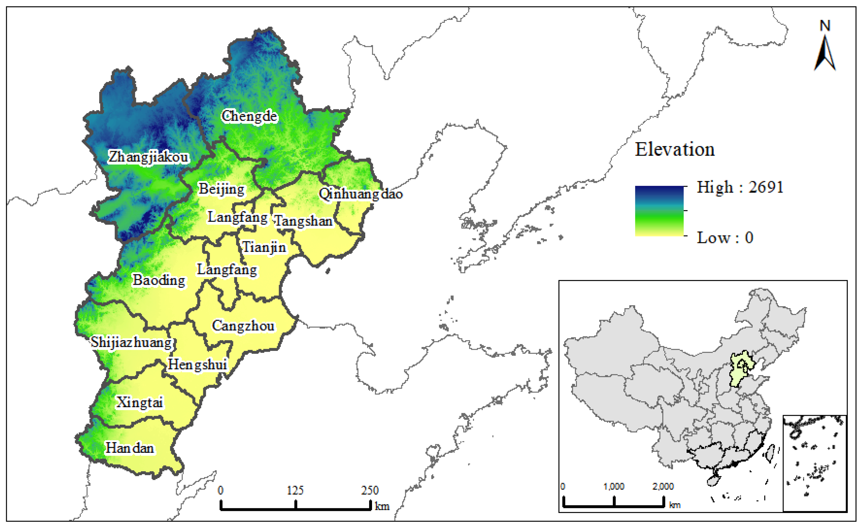
2.1. Study Area

The Beijing–Tianjin–Hebei urban agglomeration (BTHUA) lies in the center of China’s Circum–Bohai–Sea Region, with a population of 109.8 million in 2019. It covers 134,735 square kilometers, accounting for 7.79% of China’s population and 1.9% of China’s territory. In 2019, the BTHUA produced 8447 billion Yuan of GDP, accounting for 8.56% of the national GDP and ranking third among China’s 20 urban agglomerations. Its GDP per capita increased to 77,000 Yuan in 2019. The urbanization of BTHUA reached 62.13%, higher than the average national rate. The BTHUA is usually administratively divided into three distinct regions: Beijing, Tianjin, and Hebei, which include the cities of Shijiazhuang, Baoding, Langfang, Cangzhou, Qinhuangdao, Tangshan, Zhangjiakou, and Chengde. The spatial range data for this studied region is obtained from China National Natural Resources Department Standard Map Service System Pipe Network (http://bzdt.ch.mnr.gov.cn/, accessed on 5 January 2022) (Figure 1).

2.2. Natural Factors

Consistent with previous research, the natural conditions explored in this study include four factors: rainfall (R), wind speed (WS), relative humidity (RH), and temperature (T). Rainfall is a fundamental natural factor known to negatively impact PM_2.5 concentrations in Chinese cities [25], consistent also with research results from Nagasaki, Japan [26]. Using Seoul as a study area, Park (2021) found that wind speed was essential to PM_2.5 concentrations [27]. Pateraki (2012) found a significant correlation between relative humidity and PM_2.5 [28], consistent with the results of Tai (2010) [29]. Temperature is known to be sensitive to all pollutant concentrations [30]. In particular, Yang (2017) found a negative relationship between temperature and PM_2.5 concentrations [31].

Table 1. Statistical summary of the variables.

Variable Definition	Symbol	Max	Min	Mean	Std. Dev.
Rainfall (mm)	R	8483.42	4881.53	6083.97	744.85
Wind speed (m/s)	WS	2.59	1.88	2.25	0.21
Relatively humidity (%)	RH	64.38	50.17	57.90	3.19
Temperature (°C)	T	13.87	9.18	12.31	1.30
Economic development (billion yuan)	GDP	3537.13	122.00	623.14	813.96
Industrial structure (%)	IS	0.57	0.16	0.41	0.10
Technology innovation (billion yuan)	TI	223.36	0.01	13.75	37.96
Foreign Direct Investment (billion dollar)	FDI	24.33	0.01	2.47	4.71
Environmental regulation (ton/billion yuan)	ER	7.89	0.01	1.12	1.41
Urbanization (%)	UR	86.60	46.64	59.53	11.72

shows the statistical information for each of the variables related to PM_2.5.

2.3. Socioeconomic Factors

Based on previous research, we selected a wide range of anthropological influencing factors related to PM_2.5 concentrations [32,33,34]. A set of relevant determinants of PM_2.5 were selected scientifically and rationally by extending existing analytical frameworks. We examined six variables: economic development, industrial structure, technology innovation, foreign direct investment, government regulation, and urbanization, all of which have been frequently applied to analyze PM_2.5 concentrations. First, as a common indicator of economic development, the increase in GDP in China has mainly been driven by fossil fuel consumption, which can produce large amounts of air pollution. Second, secondary industry, consisting of both labor-intensive and energy-intensive industries, led to an increase in PM_2.5 concentrations. We took the proportion of secondary industry as a proxy for industry structure, which is expected to be positively correlated with PM_2.5 concentrations. Third, foreign direct investment has a contentious relationship with PM_2.5 concentrations levels. On the one hand, FDI offers low-pollution equipment and technologies and better management, understood to result in reduced emissions. On the other hand, FDI may contribute to increased PM_2.5 concentrations according to the pollution haven hypothesis. Next, technological innovation is used because technological progress reduces energy consumption and PM_2.5 concentrations. Government regulation also plays an important role in controlling PM_2.5 concentrations. The more strict anti-pollution countermeasures carried out by the government, the lower the PM_2.5 emissions. In addition, it is generally argued that rapid urbanization may negatively impact ambient air quality because urbanization usually requires more extensive infrastructure and transportation, which fosters more fossil fuel consumption and higher PM_2.5 concentration.

Data regarding factors influencing PM_2.5 concentrations from 2015 to 2019 were obtained from various sources, including the Beijing Statistical Yearbook, Tianjin Statistical Yearbook, Hebei Statistical Yearbook, China Regional Economic Statistical Yearbook, China Urban Statistical Yearbook, China Science and Technology Statistical Yearbook (CNKI: http://data.cnki.net/Yearbook, accessed on 5 January 2022). These indicators are summarized in Table 1.

2.4. PM_2.5 Data

This paper chose the BTHUA as the study area, with PM_2.5 concentration data derived from China’s National Environmental Monitoring Centre (http://106.37.208.233:20035/, accessed on 5 January 2022). The data quality control for PM_2.5 was performed based on the GB3095-2012 requirements of China’s National Ambient Air Quality Standards (AAQS) to validate air pollutant concentration data. In this study, the monitored 24-h averaged PM_2.5 concentrations at all the stations in a city represent the polluted level of the city. According to the definition of GB3095-2012, the “daily average” refers to the arithmetic mean of a natural daily 24-h average concentration, while the “monthly average” refers to the arithmetic average of the mean concentrations of each day in a calendar month; the “seasonal average” represents the arithmetic average of the mean concentrations of each day in a calendar quarter, while the “annual (yearly) average” represents the arithmetic average of the mean concentrations of each day in a calendar year; here, spring covers March through May, summer spans June through August, autumn indicates September through November, and winter consists of December, January, and February.

2.5. Geographically and Temporally Weighted Regression (GTWR) Modeling

A geographically and temporally weighted regression (GTWR) model was employed to observe the influence of factors on the explained variables by considering the spatial position relationship between variables, which could capture the instability and mutual differences of spatial data; however, the effect of time would be largely ignored. The GTWR is derived from the local spatiotemporal coefficient of the variation model proposed by Huang (2010) [35], which is a spatiotemporal analysis method based on a GWR model incorporated time series and has the advantage of a time-weighted regression (TWR) in identifying temporal effects. Meanwhile, there is no need to consider the problem of a limited quantity of samples. The spatiotemporal weight matrix is constructed according to the three-dimensional coordinates in this model. An analysis region closer to the region defined by the coordinates is defined to have greater weight (including the proximity of time and space) [36]. A spherical region constructed with the analysis region as the sphere’s center is used for local regression. Then, the parameter estimates for different regions at different times are considered. This method has been used in several studies. Wang et al. (2021) employed the geographically and temporally weighted regression model to analyze the varying importance and spatiotemporal differentiation of the factors influencing ecosystem services in the Pearl River Delta of China [37]. Liang et al. (2019) studied the impact of urbanization factors and subsystems on environmental pollution by using a GTWR model [38]. The exact calculation process is as follows

$$\begin{gathered} y_i={\beta }_0(lon{g}_i,la{t}_i,t_i)+{\displaystyle \sum _j^n{\beta }_j}(lon{g}_i,la{t}_i,t_i)x_{ij}+{\epsilon }_i \\ i=1,2,3,\cdots ,13 j=1,2,3,\cdots ,n \end{gathered}$$

(1)

Here, $y_i$ is the PM_2.5 concentration of city $i$, $lon{g}_i$ is the longitude of the city $i$, $la{t}_i$ is the latitude of the city $i$, $t_i$ is the year of the city $i$, ${\beta }_0(lon{g}_i,la{t}_i,t_i)$ and ${\beta }_j(lon{g}_i,la{t}_i,t_i)$ are the latitude and longitude function of city $i$, and the parameters to be estimated. The term $x_{ij}$ is the explanatory variable of the city factors to PM_2.5, and ${\epsilon }_i\stackrel{iid}{\sim }N(0,{\sigma }^2)$ is the random disturbance term.

The space–time weighted matrix is a key part of GTWR model, and the formulation is: $W(lon{g}_i,la{t}_i,t_i)=diag(w_{i1},w_{i2},\cdots ,w_{im})$, $m=1,2,3,\cdots ,13$; $w_{im}$ is a function based on the space–time distance attenuation

$$w_{im}=\exp (-\frac{d_{im}^2}{h^2})$$

(2)

where $d_{im}$ is the spatiotemporal distance between $i$ and $m$, and $h^2$ is the width of the spatiotemporal window. The term d_im and the minimum cross-verification method is determined by

$$d_{im}=\sqrt{\lambda [{(lon{g}_i-lon{g}_m)}^2+{(la{t}_i-la{t}_m)}^2]+\gamma {(t_i-t_m)}^2}$$

(3)

$$\min CV={\displaystyle \sum [y_i-\stackrel{\wedge }{y_{m\ne i}(h)}}]$$

(4)

where $\lambda$ determines the spatial distance ${(lon{g}_i-lon{g}_m)}^2+{(la{t}_i-la{t}_m)}^2$, when $\lambda =0$ there is no spatial effect; $\gamma$ determines the separation in time ${(t_i-t_m)}^2$, when $\gamma =0$ there is no time effect. The GTWR model requires $\lambda \ne 0$ and $\gamma \ne 0$; $h$ is the optimal time–space window width determined by the cross-verification method (CV) by minimizing the sum of the squares of residuals.

Letting $h^{s-t}$ be the width of the space–time window, $h^s$ be the width of the spatial window, $h^t$ be the width of the time window, and satisfy $h^{s-t}$ = $\lambda h^s$ = $\gamma h^t$. At this point, substituting Equations (3) and (4) into Equation (2), we obtain

$$w_{im}^{st}=\exp [-\frac{{(lon{g}_i-lon{g}_m)}^2+{(la{t}_i-la{t}_m)}^2}{{(h^s)}^2}-\frac{{(t_i-t_m)}^2}{{(h^t)}^2}]$$

(5)

Equation (5) is simplified and can be obtained as follows

$$w_{im}^{st}=w_{im}^{st}=\exp [-\frac{{(lon{g}_i-lon{g}_m)}^2+{(la{t}_i-la{t}_m)}^2}{{(h^s)}^2}]*\exp [-\frac{{(t_i-t_m)}^2}{{(h^t)}^2}]=w_{im}^s*w_{im}^t$$

(6)

Bandwidth plays a significant role in the regression results and this paper adopts an adaptive bandwidth and establishes the AICc as its criterion to obtain more accurate analysis, given that excessive bandwidth results in points with little impact in the fitting process, while a bandwidth too small produces overfitting. To facilitate differentiation, this paper divides the influence degree types according to the parameter results and divides the negative and positive influences into low, medium, and high categories, respectively.

3. Results

3.1. Characteristics of Temporal and Spatial Variation to PM_2.5

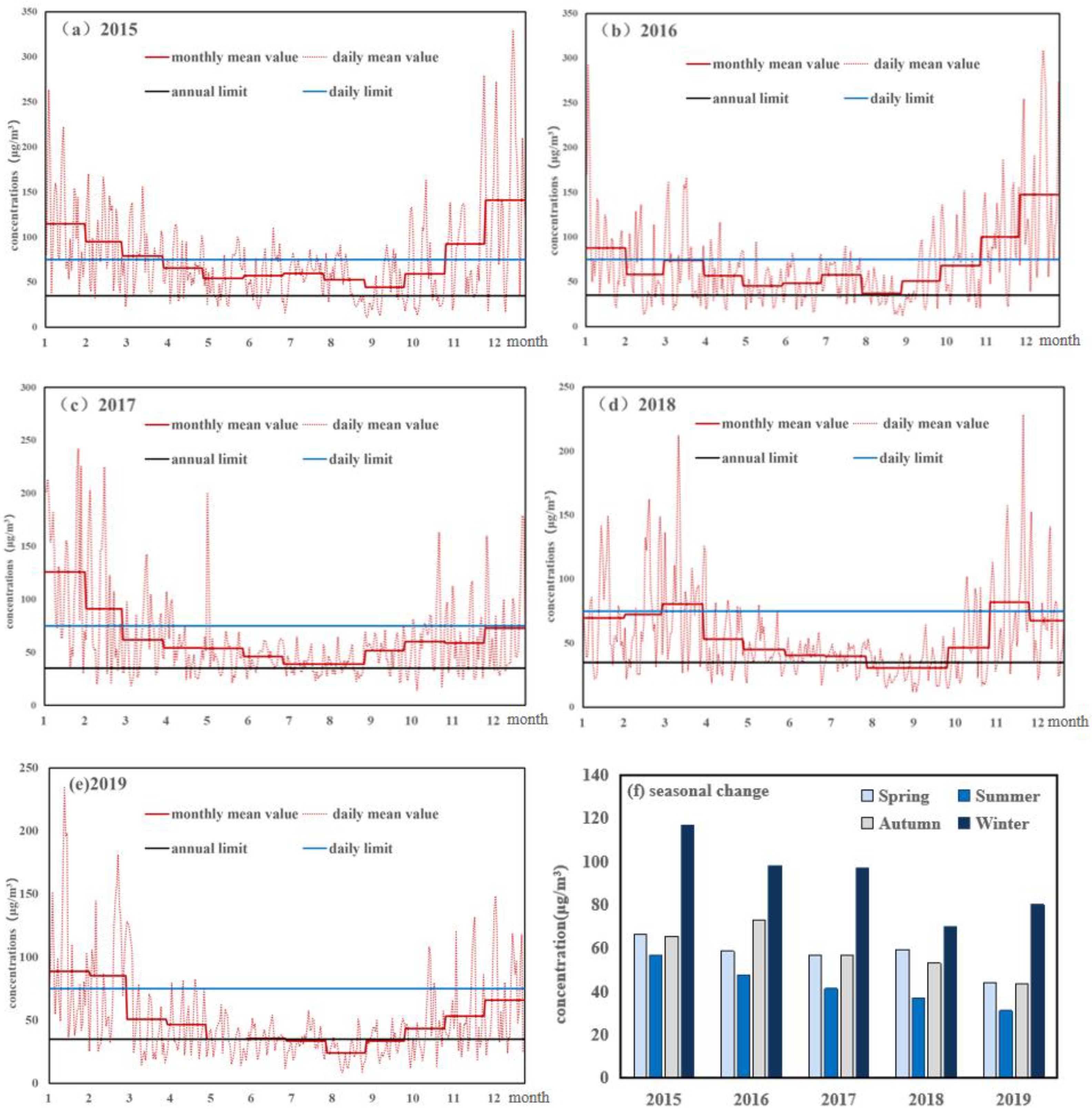
3.1.1. Temporal Characteristics

The PM_2.5 concentration measurements covered the five years from 2015 to 2019. Figure 2 shows the 24-h and monthly measurements of PM_2.5 concentrations over this time and generally indicates that PM_2.5 concentrations remarkably exceeded the Chinese standard of 35 μg/m³ (black line). Obviously, more often than not, monthly averages exceeded the standard of 75 μg/m³ (blue line). The PM_2.5 concentrations achieved their highest level in 2015 before decreasing in the following years. In total, 1325 days out of 1826 days met the criteria, while the remaining 501 days went beyond the criteria, ranging from 35 μg/m³ to 310 μg/m³. The 24-h averages of PM_2.5 displayed cyclic variations over certain time intervals in BTHUA (Figure 2). The average length of a PM_2.5 cycle was almost seven days, both in spring and winter, while that of summer and autumn was almost twice as long, about 15 days. The 24-h maximum value occurred on 22 December 2015 at 329.84 μg/m³, while the minimum was recorded on 13 August 2019, at 8.76 μg/m³.

Figure 2 demonstrates the monthly averages of PM_2.5 concentration over 12 months for each year from 2015 to 2019, which illustrates distinct variations. The monthly averages were similar in every year and showed a U-shaped pattern. The highest concentration occurred between October and March, and the lowest concentrations were clustered between May and September. The highest monthly average value was December, at 99 μg/m³. The lowest value was observed in August (36.7 μg/m³), still slightly higher than the AAQ standards.

The highest value of PM_2.5, with an average value exceeding 92 μg/m³, appeared in winter when centralized heating was ongoing. The average value for the winter season was 116.9 μg/m³ in 2015, whereas after that year, there was a clear decline that became more profound in 2018 with the lowest value, followed by a slight increase in 2019, with an average value of around 80 μg/m³. Autumn and spring ranked second and third with mean values of 58.4 μg/m³ and 57.0 μg/m³, respectively. The lowest concentrations occurred in summer, with an average value of 42.7 μg/m³. Notably, none of the average seasonal values met the Ambient Air Quality Standards (Figure 2f).

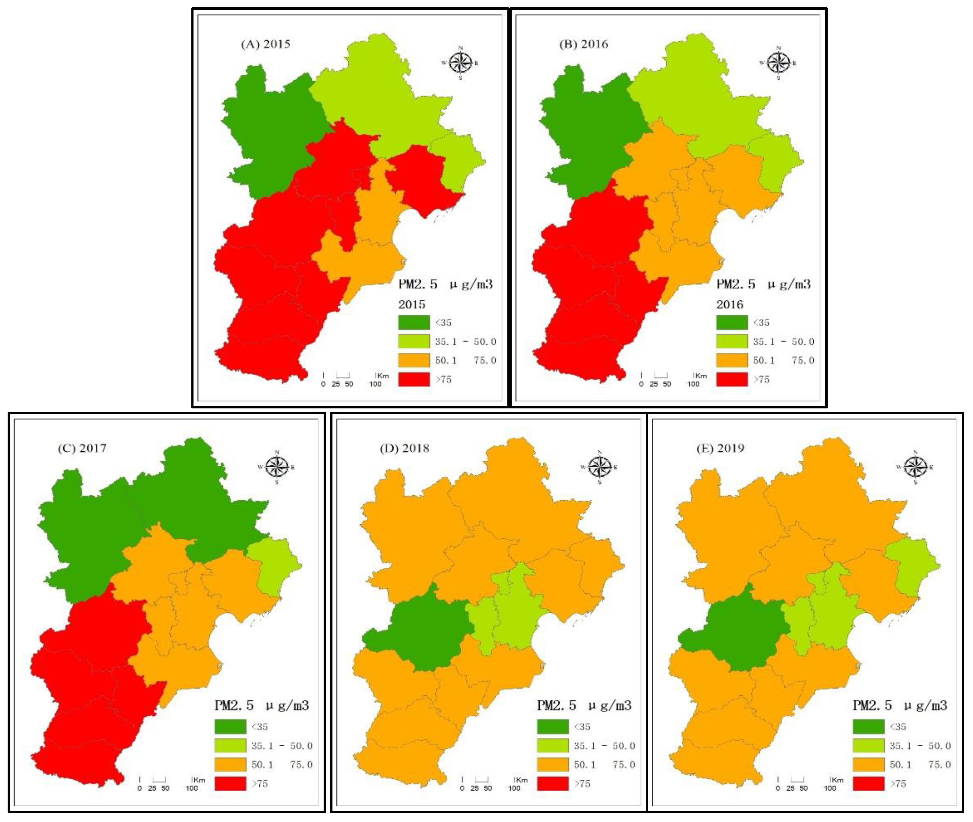
3.1.2. Spatial Change

Figure 3 shows the markedly changed magnitude and spatial distribution of PM_2.5 concentrations in the BTHUA from 2015 to 2019. According to both the World Health Organization (WHO) and China’s national ambient air quality standards (AAQA), we established five annual PM_2.5 level ranges, including excellent (<15 μg/m³), good (15–35 μg/m³), slightly polluted (35–50 μg/m³), moderately polluted (50–75 μg/m³), and heavily polluted (>75 μg/m³). As seen in Figure 3, there were no cities with concentrations lower than 15 μg/m³ from 2015 to 2019. In 2015, the areas with heavily polluted levels (i.e., mean annual PM_2.5 > 75 μg/m³) were clustered around the middle and southern part of BTHUA, while the value of PM_2.5 concentrations was relatively lower (<50 μg/m³) in the northern mountain areas. In 2015, eight cities, including Beijing, Langfang, Tangshan, Baoding, Shijiazhuang, Xingtai, Hengshui, and Handan, exceeded the heavily polluted level, accounting for 72.72% of the whole area. During 2016 and 2017, Beijing and Tangshan were excluded from the heavily polluted list and, consequently, the number of heavily polluted areas decreased. Compared with previous years, the gap between heavily polluted areas has narrowed between the northern and southern regions since 2018. In other words, PM_2.5 concentrations in most of the northern regions increased from “good” or “slightly polluted” to the “moderately polluted” level, while those of the southern regions decreased from “heavily polluted” to the “moderately polluted” level. In particular, Baoding had the lowest PM_2.5 concentrations after 2018, which may be due to the national strategic establishment of a “Xiong’An New Area”, which, as one of three national strategies, has made Baoding area undertake the important role of the so-called non-capital functions to take over the heavy burdens the capital city of Beijing once bore.

3.2. Factors Influencing PM_2.5 Concentrations

We chose ten variables to determine the mechanisms that influenced the PM_2.5 concentrations in BTHUA across the study period. Early studies have clearly established a significant spatial autocorrelation of the PM_2.5 distribution in the BTHUA area. The clustering characteristics reflect the spatial spillover effect of PM_2.5 concentrations, meaning that local PM_2.5 pollution can positively impact concentrations in adjacent areas [39,40]. The GTWR model was extended from a GWR model to take temporal variations into consideration, allowing significantly better goodness of fit than that of conventional least square methods and GWR models [20]. To explore the spatial and temporal non-stationary nature of the mechanism, a geographic and time-weighted regression (GTWR) model was constructed to analyze the spatial and temporal differentiation of the influencing factors from 2015 to 2019. The results from

Table 2. Assessment of GTWR model.

Indicator	Model Type			Model Comparison
	OLS	GWR	GTWR	GTWR–OLS	GTWR–GWR
AICc	339.27	287.65	269.73	−69.54	−17.92
R2	0.823	0.921	0.948	0.125	0.027

showed that, in comparison with OLS and GWR, the AICc value of GTWR produced better fitting effects with decreases by 69.54 and 17.92, and R² increases by 0.125 and 0.027, respectively. The test suggested that the GTWR model performed better than the global OLS and GWR model. When analyzing the influencing factors of PM_2.5 concentrations, the GTWR model containing spatial and temporal heterogeneity is more compatible than the OLS model, which focuses only on global regression and the GWR model without any time effects.

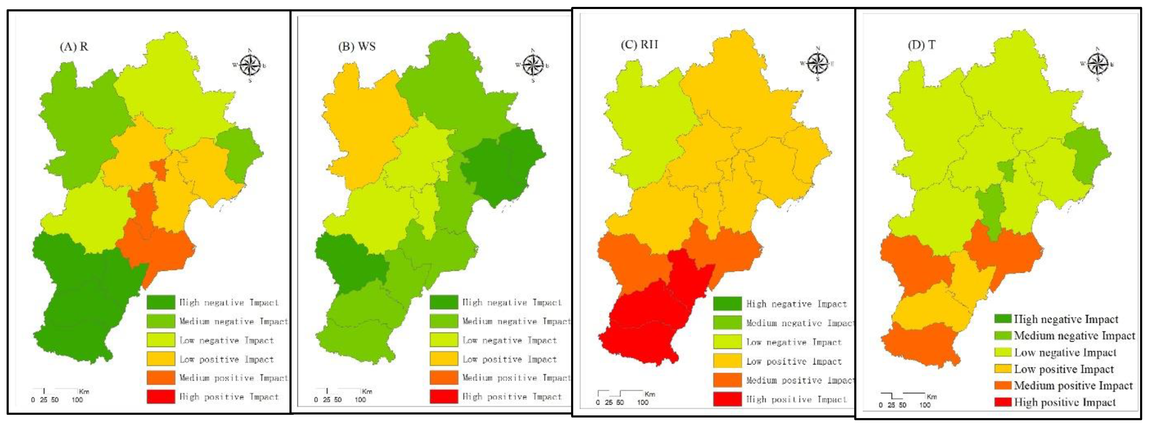
3.2.1. Natural Factors Influencing PM_2.5 Concentrations

Figure 4 shows the spatial differences present in the coefficients of the natural factors addressed in the BTHUA. The results indicate a negative regression coefficient between rainfall and PM_2.5 concentrations. The negative regression coefficient between the wind speed and PM_2.5 concentrations was about 92.31%. In most cities, the factor of relative humidity correlated positively with PM_2.5 concentrations (92.31%). In contrast, the temperature factor displayed a negative relationship with PM_2.5 concentrations (61.54%).

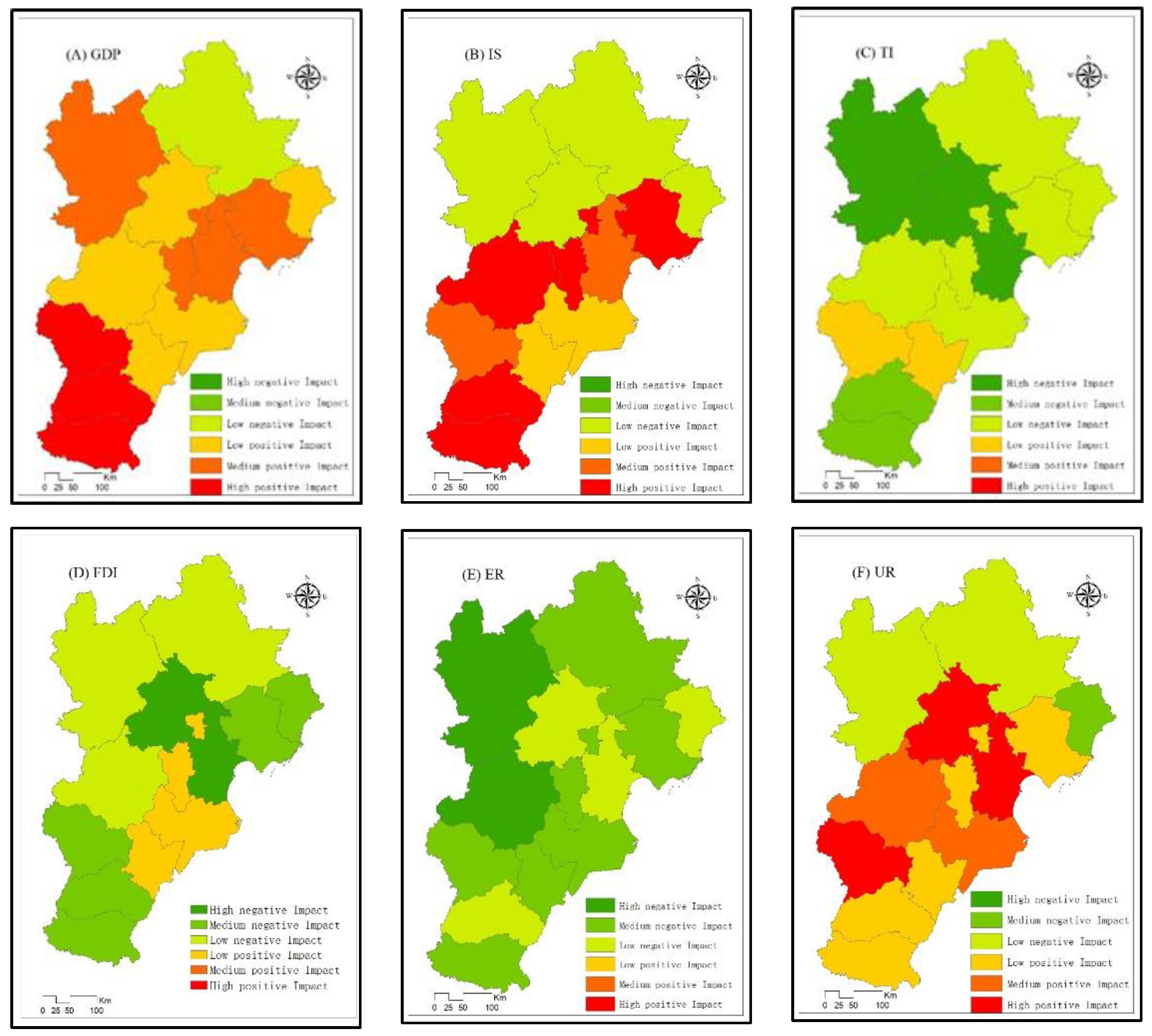
3.2.2. Socioeconomic Factors Influencing PM_2.5 Concentrations

Figure 5 illustrates the geographic distribution of the regression coefficient values for the socioeconomic factors of this study. Previous research has highlighted the GDP and industry structure as significant factors affecting PM_2.5 concentrations. Data analysis revealed a positive correlation coefficient between GDP and PM_2.5 concentrations of about 92.31% for this area. The regression results for the GTWR show that the positive regression coefficient between the space proportion dedicated to industrial structures and PM_2.5 is about 69.23%. The area of BTHUA with a positive correlation coefficient between the urbanization factor and PM_2.5 concentrations accounted for about 76.92% of the total area.

About 84.62% of the area in the BTHUA was characterized by negative correlation coefficients between the technology innovation factor and PM_2.5 concentrations. The total effect of foreign direct investment on PM_2.5 concentrations is also proven to be negative, with a regression coefficient of 76.92%, the reason for which may be interpreted by the pollution halo hypothesis. The environmental regulation factor in the BTHUA demonstrated a distinct negative correlation with PM_2.5 concentrations, which was consistent with both initial predictions and common sense.

4. Discussion

Our results indicate significant spatial heterogeneity in both the direction and strength of the determinants at the local scale. In the southern part of the BTHUA, such as the cities of Shijiazhuang, Xingtai, Handan, PM_2.5 concentrations had a high positive correlation with economic growth (Figure 5a). According to the environmental Kuznets curve, economic development can, in its later stages, be harmful to the environment because it consumes large amounts of resources and energy. It seems paradoxical that a mutualistic relationship between China’s economic growth and environmental pollution has likely long existed until the BTHUA broke through the inflection point of the environmental Kuznets curve [41].

The PM_2.5 concentrations showed strong positive correlations with the secondary industrial structure (Figure 5b). The economy in the four areas of Tianjin, Tangshan, Shijiazhuang, and Xingtai was driven mainly by heavy industries such as steel, automobile, and equipment manufacturing facilities, characterized by high resource consumption. Heavy industry served as the chief source of PM_2.5 concentrations in these areas. On the contrary, the industrial structure of Zhangjiakou, Chengde, Qinhuangdao, and Beijing in the north correlated negatively with the concentrations of PM_2.5. The reason lies within the fact that the main industrial structure of these places is dominated by the service industry, with relatively less pollution from industrial activities. For example, Beijing is famous for its tertiary and technology-intensive industries, both of which are classified as service industries resulting in less energy consumption. As an ecological barrier of the Beijing–Tianjin–Hebei urban agglomeration, the northern mountainous area has emphasized the development of the tourism-driven industry. Therefore, we can conclude that different industrial structures produce different effects on the environmental quality of cities.

Technology innovation was negatively correlated with PM_2.5 concentrations (Figure 5c). For one, this may be due to the continuous creation of new technologies and products that are more environmentally friendly and efficient to both economic activities and daily life. For another, the pollution prevention technology in China is becoming more advanced so that air pollution can be better controlled. In megacities such as Beijing and Tianjin, where there is a tremendous emphasis on scientific research and technological improvements, more and more technicians and workers are receiving high-level technical education, which tends to explain the strong negative correlation between technical innovation levels and PM_2.5 concentrations. In contrast, the TI levels of Shijiazhuang, which is in the transformation stage of the pollution industry, and Hengshui, which is lagging in technological innovation because of its relatively poor economic development, have a positive correlation with PM_2.5 concentration, indicating that its technological achievement may not, as of yet, have been transformed into actual ecological benefits.

The foreign direct investment significantly reduces PM_2.5 concentrations, especially if the FDI is accompanied by advanced technologies, which would tend to create spillovers for domestic industries. Beijing and Tianjin showed large negative coefficients between FDI and PM_2.5 concentrations (Figure 5d). Wang et al. (2020) researched 18 urban agglomerations in China and found that FDI had a negative impact on the BTHUA, which is consistent with the research results of this paper [42].

The environmental regulation factor in the BTHUA showed a distinct negative correlation with PM_2.5 concentrations (Figure 5e). This conclusion is further evidenced in the goalsetting of “constructing ecological civilization,” a section of the report by the 18th National Congress of the Communist Party of China (CPC). Consequently, government regulators began to take powerful measures to enhance economic and social transformation based on the efficient use of resources and establishing green, low-carbon growth, upgrading production, and changing lifestyles to achieve the goal of green development. Qu (2020) pointed out that the aggressive abatement policies likely contributed to reductions in normalized PM_2.5 concentrations [43].

The positive coefficients of megacities and big cities such as Beijing, Tianjin, and Shijiazhuang are high, which indicates that the intensive urbanization in these areas intensifies environmental pollution (Figure 5f). Negative coefficients between urbanization and PM_2.5 emerged mainly in the northern mountainous areas. We can conclude that suitable urbanization in mountainous areas in its early stages effectively contributes to improving environmental quality. This conclusion is consistent with the research findings of Liang et al. (2019) and confirms that the impact mechanism of urbanization on PM_2.5 pollution varies with the level of urban development [38].

5. Conclusions

This research set out to discover the key effective influencing factors contributing to PM_2.5 in BTHUA. We analyzed the spatiotemporal change in PM_2.5 concentrations in the Beijing–Tianjin–Hebei urban agglomeration (BTHUA). We found that the PM_2.5 pollution showed an overall decreasing trend from 2015 to 2019 and the spatial gap between the north and the south decreased in recent years.

This study creatively applied an improved GWR model to a designated region so as to estimate the association between PM_2.5 concentrations and a series of key socioeconomic and meteorological factors. The GTWR model was extended from a GWR model by adding temporal variations, and the added complexity of the GTWR model produced significantly better goodness of fit than that of conventional OLS methods and GWR models. The GTWR performed in this study is helpful in recognizing the effects of influencing factors varying in time and space.

The findings of this study provide detailed empirical evidence for regions to improve air quality in accordance with local conditions. Moreover, this study contributes valuable insights to visualizing those spatial and temporal variations in the correlation coefficients of each determinant related to PM_2.5 concentrations. This visualization may help local policymakers adopt specific policies in accordance with local pollution patterns and corresponding development models, as opposed to a “one-size fits all” approach. Additionally, the cities of BTHUA should scientifically adjust industrial structures, implement the optimization and upgrading of economic growth, maximize the efficiency of energy use, implement strict environmental access standards, and define a bottom line for ecological protection.

However, there are two limitations in this paper. Due to the limited data of the socioeconomic factors, taking a city as the basic research unit restrained the choices of factor variables and further deep explorations. Future improvement should be directed to lower-level administrative regions as its basic research unit. In addition, this paper adopted the GTWR model that captures the spatial variations in regression coefficients for different research units and allows the spatiotemporal disparities. Although it has been previously used, there are still some uncertainties in its objectivity and timeliness. Hybrid deep learning methodologies such as random forest regression should be proposed in the future.

References

1. Rohde, R.A.; Muller, R.A. Air Pollution in China: Mapping of Concentrations and Sources. PLoS ONE 2015, 10, e0135749. [Google Scholar] [CrossRef]
2. Pey, J.; Alastuey, A.; Querol, X. PM10 and PM2.5 sources at an insular location in the western Mediterranean by using source apportionment techniques. Sci. Total Environ. 2013, 456, 267–277. [Google Scholar] [CrossRef] [PubMed]
3. Wang, Z. Satellite-Observed Effects from Ozone Pollution and Climate Change on Growing-Season Vegetation Activity over China during 1982–2020. Atmosphere 2021, 12, 1390. [Google Scholar] [CrossRef]
4. Lee, J.Y.; Jo, W.K.; Chun, H.-H. Long-Term Trends in Visibility and Its Relationship with Mortality, Air-Quality Index, and Meteorological Factors in Selected Areas of Korea. Aerosol Air Qual. Res. 2015, 15, 673–681. [Google Scholar] [CrossRef]
5. Wang, Z.B.; Fang, C.L. Spatial-temporal characteristics and determinants of PM2.5 in the Bohai Rim Urban Agglomeration. Chemosphere 2016, 148, 148–162. [Google Scholar] [CrossRef]
6. Hajiloo, F.; Hamzeh, S.; Gheysari, M. Impact assessment of meteorological and environmental parameters on PM2.5 concentrations using remote sensing data and GWR analysis (case study of Tehran). Environ. Sci. Pollut. Res. 2019, 26, 24331–24345. [Google Scholar] [CrossRef] [PubMed]
7. Jedruszkiewicz, J.; Czernecki, B.; Marosz, M. The variability of PM10 and PM2.5 concentrations in selected Polish agglomerations: The role of meteorological conditions, 2006–2016. Int. J. Environ. Health Res. 2017, 27, 441–462. [Google Scholar] [CrossRef]
8. Li, W.G.; Duan, F.K.; Zhao, Q.; Song, W.W.; Cheng, Y.; Wang, X.Y.; Li, L.; He, K.B. Investigating the effect of sources and meteorological conditions on wintertime haze formation in Northeast China: A case study in Harbin. Sci. Total Environ. 2021, 801, 149631. [Google Scholar] [CrossRef]
9. Wang, Q.; Kwan, M.P.; Zhou, K.; Fan, J.; Wang, Y.F.; Zhan, D.S. The impacts of urbanization on fine particulate matter (PM2.5) concentrations: Empirical evidence from 135 countries worldwide. Environ. Pollut. 2019, 247, 989–998. [Google Scholar] [CrossRef]
10. Zhou, C.S.; Wang, S.J.; Wang, J.Y. Examining the influences of urbanization on carbon dioxide emissions in the Yangtze River Delta, China: Kuznets curve relationship. Sci. Total Environ. 2019, 675, 472–482. [Google Scholar] [CrossRef]
11. Wu, W.; Zhang, M.; Ding, Y. Exploring the effect of economic and environment factors on PM2.5 concentration: A case study of the Beijing-Tianjin-Hebei region. J. Environ. Manag. 2020, 268, 110703. [Google Scholar] [CrossRef]
12. Wolde-Rufael, Y.; Idowu, S. Income distribution and CO2 emission: A comparative analysis for China and India. Renew. Sustain. Energy Rev. 2017, 74, 1336–1345. [Google Scholar] [CrossRef]
13. Wu, S.W.; Deng, F.R.; Niu, J.; Huang, Q.S.; Liu, Y.C.; Guo, X.B. Association of Heart Rate Variability in Taxi Drivers with Marked Changes in Particulate Air Pollution in Beijing in 2008. Environ. Health Perspect. 2010, 118, 87–91. [Google Scholar] [CrossRef] [PubMed] [Green Version]
14. Xie, Z.; Li, Y.; Qin, Y. Allocation of control targets for PM2.5 concentration: An empirical study from cities of atmospheric pollution transmission channel in the Beijing-Tianjin-Hebei district. J. Clean. Prod. 2020, 270, 122545. [Google Scholar] [CrossRef]
15. Zoundi, Z. CO2 emissions, renewable energy and the Environmental Kuznets Curve, a panel cointegration approach. Renew. Sustain. Energy Rev. 2017, 72, 1067–1075. [Google Scholar] [CrossRef]
16. Al-mulali, U.; Tang, C.F. Investigating the validity of pollution haven hypothesis in the gulf cooperation council (GCC) countries. Energy Policy 2013, 60, 813–819. [Google Scholar] [CrossRef]
17. Wang, S.J.; Liu, X.P.; Zhou, C.S.; Hu, J.C.; Ou, J.P. Examining the impacts of socioeconomic factors, urban form, and transportation networks on CO2 emissions in China’s megacities. Appl. Energy 2017, 185, 189–200. [Google Scholar] [CrossRef]
18. Lou, C.R.; Liu, H.Y.; Li, Y.F.; Li, Y.L. Socioeconomic Drivers of PM2.5 in the Accumulation Phase of Air Pollution Episodes in the Yangtze River Delta of China. Int. J. Environ. Res. Public Health 2016, 13, 928. [Google Scholar] [CrossRef] [Green Version]
19. Zhan, D.; Kwan, M.-P.; Zhang, W.; Yu, X.; Meng, B.; Liu, Q. The driving factors of air quality index in China. J. Clean. Prod. 2018, 197, 1342–1351. [Google Scholar] [CrossRef]
20. Liu, Q.Q.; Wu, R.; Zhang, W.Z.; Li, W.; Wang, S.J. The varying driving forces of PM2.5 concentrations in Chinese cities: Insights from a geographically and temporally weighted regression model. Environ. Int. 2020, 145, 106168. [Google Scholar] [CrossRef]
21. Li, G.D.; Fang, C.L.; Wang, S.J.; Sun, S. The Effect of Economic Growth, Urbanization, and Industrialization on Fine Particulate Matter (PM2.5) Concentrations in China. Environ. Sci. Technol. 2016, 50, 11452–11459. [Google Scholar] [CrossRef] [PubMed]
22. Wang, J.Y.; Wang, S.J.; Li, S.J. Examining the spatially varying effects of factors on PM2.5 concentrations in Chinese cities using geographically weighted regression modeling. Environ. Pollut. 2019, 248, 792–803. [Google Scholar] [CrossRef] [PubMed]
23. Akbal, Y.; Ünlü, K.D. A deep learning approach to model daily particular matter of Ankara: Key features and forecasting. Int. J. Environ. Sci. Technol. 2021, 1–17. [Google Scholar] [CrossRef]
24. Akdi, Y.; Gölveren, E.; Ünlü, K.D.; Yücel, M.E. Modeling and forecasting of monthly PM2.5 emission of Paris by periodogram-based time series methodology. Environ. Monit. Assess. 2021, 193, 622. [Google Scholar] [CrossRef]
25. Xu, B.; Lin, B.Q. What cause large regional differences in PM2.5 pollutions in China? Evidence from quantile regression model. J. Clean. Prod. 2018, 174, 447–461. [Google Scholar] [CrossRef]
26. Li, X.Y.; Song, H.Q.; Zhai, S.Y.; Lu, S.Q.; Kong, Y.F.; Xia, H.M.; Zhao, H.P. Particulate matter pollution in Chinese cities: Areal-temporal variations and their relationships with meteorological conditions (2015–2017). Environ. Pollut. 2019, 246, 11–18. [Google Scholar] [CrossRef]
27. Wang, J.; Ogawa, S. Effects of Meteorological Conditions on PM2.5 Concentrations in Nagasaki, Japan. Int. J. Environ. Res. Public Health 2015, 12, 9089–9101. [Google Scholar] [CrossRef]
28. Park, I.S.; Kim, S.H.; Jang, Y.W.; Park, M.S.; Lee, J.; Owen, J.S.; Cho, C.R.; Jee, J.B.; Chae, J.H.; Kang, M.S. Meteorological Characteristics during Periods of Greatly Reduced PM2.5 Concentrations in March 2020 in Seoul. Aerosol Air Qual. Res. 2021, 21, 200512. [Google Scholar] [CrossRef]
29. Pateraki, S.; Asimakopoulos, D.N.; Flocas, H.A.; Maggos, T.; Vasilakos, C. The role of meteorology on different sized aerosol fractions. Sci. Total Environ. 2012, 419, 124–135. [Google Scholar] [CrossRef]
30. Tai, A.P.K.; Mickley, L.J.; Jacob, D.J. Correlations between fine particulate matter (PM2.5) and meteorological variables in the United States: Implications for the sensitivity of PM2.5 to climate change. Atmos. Environ. 2010, 44, 3976–3984. [Google Scholar] [CrossRef]
31. Li, L.; Qian, J.; Ou, C.Q.; Zhou, Y.X.; Guo, C.; Guo, Y.M. Spatial and temporal analysis of Air Pollution Index and its timescale-dependent relationship with meteorological factors in Guangzhou, China, 2001–2011. Environ. Pollut. 2014, 190, 75–81. [Google Scholar] [CrossRef] [PubMed]
32. Yang, Q.Q.; Yuan, Q.Q.; Li, T.W.; Shen, H.F.; Zhang, L.P. The Relationships between PM2.5 and Meteorological Factors in China: Seasonal and Regional Variations. Int. J. Environ. Res. Public Health 2017, 14, 1510. [Google Scholar] [CrossRef] [Green Version]
33. Masiol, M.; Hopke, P.K.; Felton, H.D.; Frank, B.P.; Rattigan, O.V.; Wurth, M.J.; LaDuke, G.H. Source apportionment of PM2.5 chemically speciated mass and particle number concentrations in New York City. Atmos. Environ. 2017, 148, 215–229. [Google Scholar] [CrossRef]
34. Hao, Y.; Liu, Y.-M. The influential factors of urban PM2.5 concentrations in China: A spatial econometric analysis. J. Clean. Prod. 2016, 112, 1443–1453. [Google Scholar] [CrossRef]
35. Chen, J.; Zhou, C.; Wang, S.; Hu, J. Identifying the socioeconomic determinants of population exposure to particulate matter (PM2.5) in China using geographically weighted regression modeling. Environ. Pollut. 2018, 241, 494–503. [Google Scholar] [CrossRef] [PubMed]
36. Huang, B.; Wu, B.; Barry, M. Geographically and temporally weighted regression for modeling spatio-temporal variation in house prices. Int. J. Geogr. Inf. Sci. 2010, 24, 383–401. [Google Scholar] [CrossRef]
37. Wu, S.S.; Wang, Z.Y.; Du, Z.H.; Huang, B.; Zhang, F.; Liu, R.Y. Geographically and temporally neural network weighted regression for modeling spatiotemporal non-stationary relationships. Int. J. Geogr. Inf. Sci. 2021, 35, 582–608. [Google Scholar] [CrossRef]
38. Wang, S.J.; Liu, Z.T.; Chen, Y.X.; Fang, C.L. Factors influencing ecosystem services in the Pearl River Delta, China: Spatiotemporal differentiation and varying importance. Resour. Conserv. Recycl. 2021, 168, 105477. [Google Scholar] [CrossRef]
39. Liang, L.W.; Wang, Z.B.; Li, J.X. The effect of urbanization on environmental pollution in rapidly developing urban agglomerations. J. Clean. Prod. 2019, 237, 117649. [Google Scholar] [CrossRef]
40. Huang, Q.Y.; Chen, G.D.; Xu, C.; Jiang, W.Y.; Su, M.R. Spatial Variation of the Effect of Multidimensional Urbanization on PM2.5 Concentration in the Beijing-Tianjin-Hebei (BTH) Urban Agglomeration. Int. J. Environ. Res. Public Health 2021, 18, 2077. [Google Scholar] [CrossRef] [PubMed]
41. Li, H.J.; Qi, Y.J.; Li, C.; Liu, X.Y. Routes and clustering features of PM2.5 spillover within the Jing-Jin-Ji region at multiple timescales identified using complex network-based methods. J. Clean. Prod. 2019, 209, 1195–1205. [Google Scholar] [CrossRef]
42. Shahbaz, M.; Khraief, N.; Uddin, G.S.; Ozturk, I. Environmental Kuznets curve in an open economy: A bounds testing and causality analysis for Tunisia. Renew. Sustain. Energy Rev. 2014, 34, 325–336. [Google Scholar] [CrossRef] [Green Version]
43. Wang, Z.B.; Li, J.X.; Liang, L.W. Spatio-temporal evolution of ozone pollution and its influencing factors in the Beijing-Tianjin-Hebei Urban Agglomeration. Environ. Pollut. 2020, 256, 113419. [Google Scholar] [CrossRef]
Figure 1. Location and range of Beijing–Tianjin–Hebei urban agglomeration.
Atmosphere 13 00407 g001
Figure 2. Daily and monthly variations in PM2.5 concentrations in Beijing–Tianjin–Hebei urban agglomeration from 2015 to 2019.
Atmosphere 13 00407 g002
Figure 3. Spatial distribution of PM2.5 concentrations in the Beijing–Tianjin–Hebei urban agglomeration from 2015 to 2019.
Atmosphere 13 00407 g003
Figure 4. Spatial distribution of regression coefficients for natural factors in the Beijing–Tianjin–Hebei urban agglomeration during the study period.
Atmosphere 13 00407 g004
Figure 5. Spatial distribution of regression coefficients for socioeconomic factors in the Beijing–Tianjin–Hebei urban agglomeration during the study period.
Atmosphere 13 00407 g005