Abstract
This study assessed leaf fluxes of CO2, CH4 and biogenic volatile organic compounds (BVOC) for two common urban tree species, Platanus × acerifolia (exotic) and Schinus molle (native), widely distributed in Santiago, Chile. The emission factors (EF) and the Photochemical Ozone Creation Index (POCI) for S. molle and P. × acerifolia were estimated. The global EF was 6.4 times higher for P. × acerifolia compared with S. molle, with similar rates of photosynthesis for both species. Isoprene represented more than 86% of the total BVOCs leaf fluxes being 7.6 times greater for P. × acerifolia than S. molle. For P. × acerifolia, BVOCs represented 2% of total carbon fixation while representing 0.24% for S. molle. These results may suggest that plant species growing outside their ecological range may exhibit greater BVOCs leaf fluxes, proportional to photosynthesis, compared to well-adapted ones. The results found may contribute to better urban forest planning.
1. Introduction
Vegetation provides a wide range of ecosystem services in urban environments such as generating O2 and absorbing CO2, reducing soil erosion and wind speed, generating shade that reduces air temperature and capturing particulate matter (PM), among others. Hence, vegetation provides valuable services that contribute to improve air quality in cities [1]. However, trees can also emit biogenic volatile organic compounds (BVOC), which are precursors of tropospheric ozone (O3) negatively affecting human health and the environment. Volatile organic compounds (VOC) can also be of anthropic origin (AVOC) such as those from industrial processes and the combustion of motorized vehicles [2]. All plants emit BVOCs at a rate that depends on species, age, and external factors such as temperature, relative humidity, solar radiation, and stress, among others. The release of BVOC by plants may play different roles such as attracting pollinators or repelling agents of pest and diseases, acting as a countermeasure to external stimuli and a form of communication between different individuals [3].
BVOCs are common in the environment and many of them are recognized by their fragrances. These scented compounds are known as terpenes and their base unit is isoprene (C5H8), a reactive molecule with five carbon atoms and two double bonds. They react in the atmosphere with the hydroxyl radical (•OH), nitrate radical (•NO3) especially during the night, ozone and other chemical species, leading to reactions between nitrogen oxides (NOx) and organic reactive intermediates that ultimately enhance tropospheric ozone production and secondary organic aerosols (SOA), both related to different human and plant health problems [4,5,6,7]). Nowadays, high concentrations of O3 can be found in many cities due to the oxidation reactions of VOCs in the presence of NOx from combustion processes, especially motor vehicles. High concentrations carry risks such as cardio-respiratory diseases, oxidation of materials and damage to flora and fauna [6]. Tropospheric ozone moving inside the leaf through the stomata brings about the production of reactive oxygen species damaging the photosynthetic machinery [7] despite the plant’s increased production of compounds with antioxidative capacity [8]. The city of Santiago, Chile, exhibits serious problems with O3 during the spring–summer period [9,10,11]. The threshold for ozone is 120 µg m−3, considering an 8 h mobile average, being frequently exceeded during spring-summer, especially in the northeast of the city [10]. A recent work monitoring ozone concentration in eastern Santiago during the period 2010–2018 showed that on average 43 days per year were above the recommended levels and that the ozone formation regime is VOC-limited [12]. Although anthropogenic VOCs are the dominant chemical species [13], it becomes relevant to identify the sources of BVOC emissions and their potential as precursors of urban pollutants. Methane, not considered a BVOC, is only rarely measured but it might be worth comparing such fluxes against those of BVOCs. Besides, knowing the fraction that BVOCs represents in terms of carbon fixed through photosynthesis across plant species may shed light on the metabolic plant responses to stresses.
The aim of this work was to assess CH4, CO2 and BVOCs fluxes by two relatively abundant tree species in the city of Santiago, Platanus × acerifolia and Schinus molle (2.3% and 1.84% in abundance, respectively), measured during a hot dry period. In addition to emission factors (EF), the potential tropospheric O3 formation index (POCI) was also estimated. This study may contribute towards a better understanding of the trade-off between carbon sequestration and BVOCs emissions in urban trees for the central region of Chile.
2. Materials and Methods
2.1. Study Site and Sampling
The study was conducted at the Faculty of Forest Sciences and Nature Conservation of University of Chile (Lat. 33°34′10.2′′ S, Long. 70°37′48.9′′ W) located in La Pintana commune (neighborhood) in the city of Santiago. The faculty is located on a campus of about 300 ha of agricultural land, with large green areas and parks surrounding the buildings. One individual of Platanus × acerifolia (exotic) and another of Schinus molle (native) were selected. Both trees were adult, healthy (no evidence of herbivory, pests, or disease) [14,15,16] and relatively well spaced from other trees with relatively little vehicular traffic surrounding them.
The measurements of methane and CO2 fluxes were performed before the sampling of BVOCs. Each tree was sampled over 5 days with four daily measurements (n = 20) during a hot dry period. P. × acerifolia was sampled on 7, 8, 9, 12 and 13 February 2018. S. molle was sampled later in the summer on 1, 2, 5, 6 and 7 March 2018.
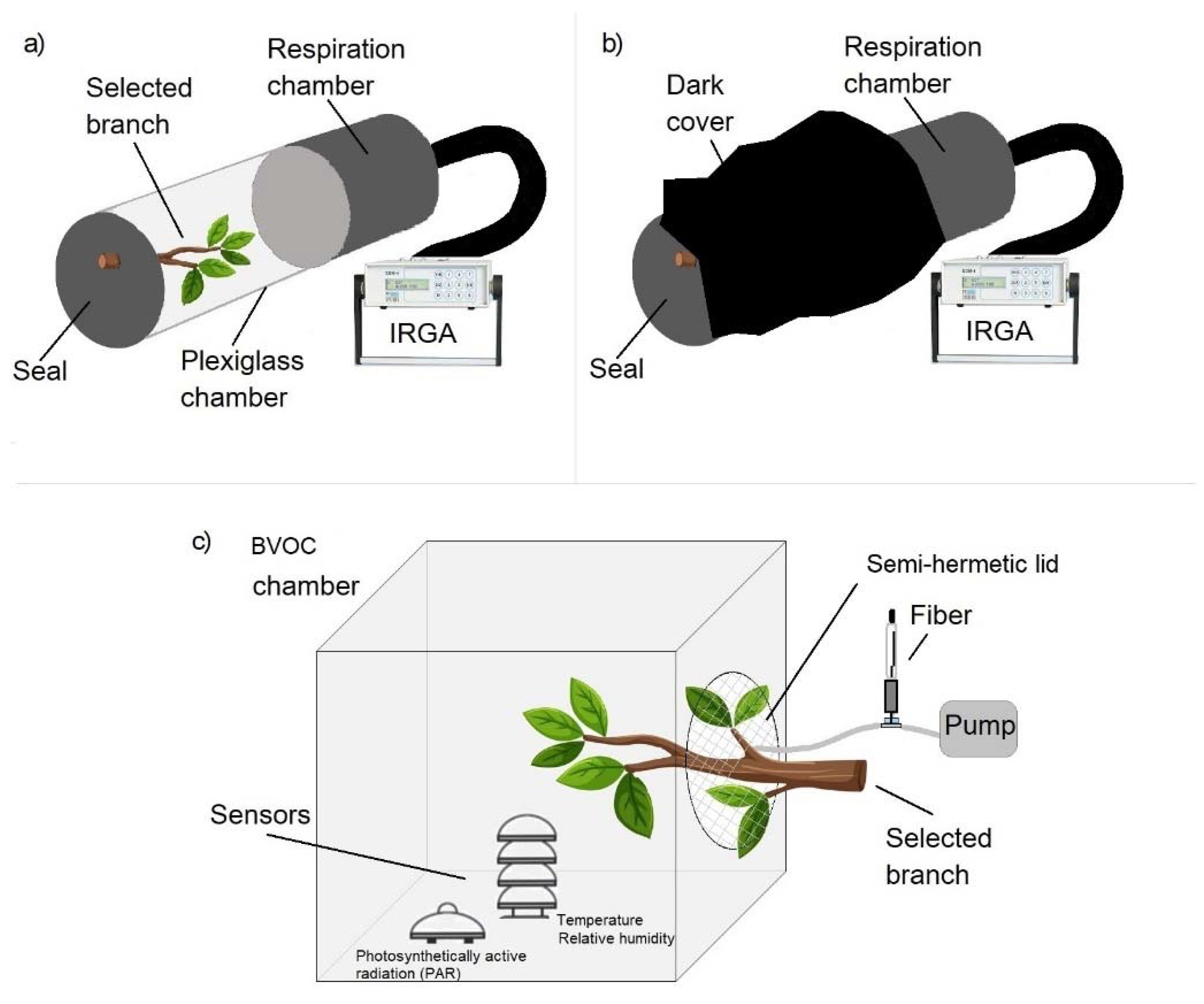
The sampling system for CO2, methane and BVOCs emitted by Platanus × acerifolia and Schinus molle is shown in Figure 1.
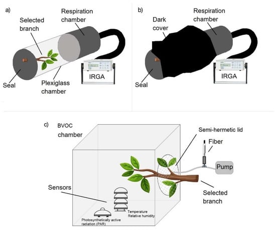
Figure 1.
Setup for sampling gases emitted by Platanus × acerifolia and Schinus molle. (a) CO2 fluxes using an Infrared Gas Analyzer (IRGA) followed by 5 min gas accumulation inside the chamber to extract a gas aliquote to determine methane concentration; (b) chamber covered with a black cloth to record autotrophic respiration; (c) Semi-closed-chamber for BVOCs sampling with sensors simultaneously recording solar radiation, temperature and relative humidity.
2.1.1. CO2 and CH4 Fluxes
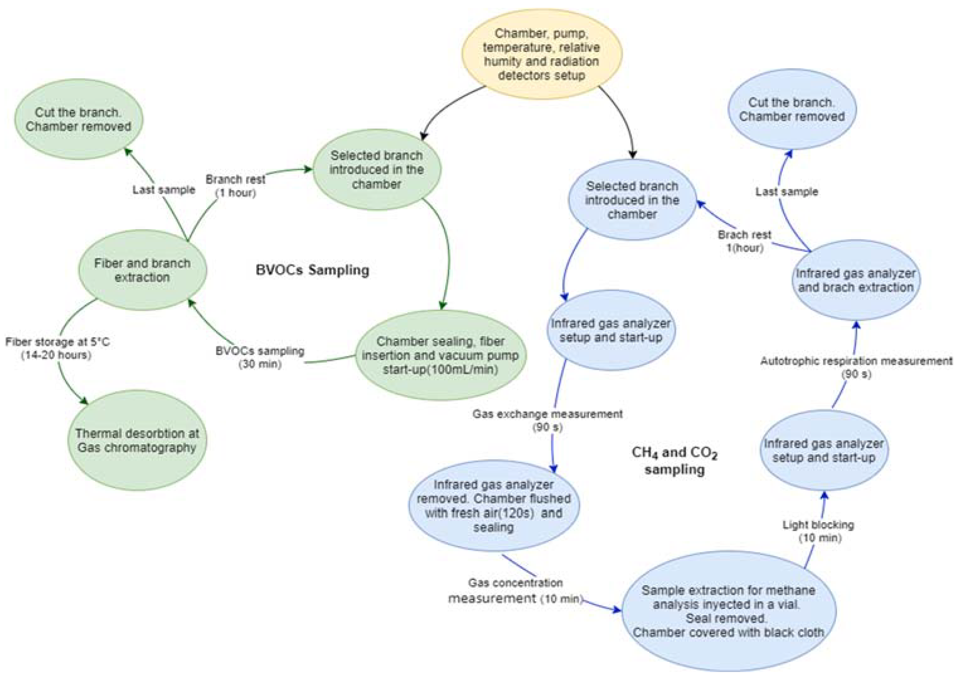
One branch per tree from the lower third of the crown but fully exposed to the sun for most of the day was sampled. The branches sampled were selected to fit inside the chamber in which gas exchange was measured. The static Plexiglas Chamber (100 mm inner diameter, 300 mm length) with a stopcock on top was used and connected to a soil respiration chamber (100 mm inner diameter, 200 mm length), Model SRC-1, PP Systems, Amesbury, MA, USA, with a total volume of 3.527 cm3 linked to an infrared gas analyzer Model EGM-4, PP Systems, Amesbury, MA, USA. Air temperature, relative humidity (PASS VP-3, Decagon Devices, Pullman, WA, USA) and solar radiation (PYR, Decagon Devices, 380–1120 nm) were continuously measured and recorded using a data logger (Decagon Devices, Model Em50). Plant CO2 and CH4 fluxes were measured in the light (photosynthesis) (Figure 1a). Each measurement was taken over 90 s. For plant CH4 fluxes, the closed chamber (volume 2.356 cm3) was sealed for 300 s before extracting a gas sample using polyethylene syringes fitted with nylon stopcocks (25 mL) and injected into pre-evacuated 12 mL vials (Exetainers, Labco Ltd., Lampeter, Wales, UK). Figure 2 shows the measurements procedure (circles in blue). Methane concentrations were determined by gas chromatography (Perkin Elmer model Clarus 600 with FID detector) at the Soils Laboratory of Universidad de Concepción, Chillán, Chile (details in SM).

Figure 2.
Measurements procedure for sampling BVOCs (green circles), CO2 and methane (blue circles); with a common step to both procedures in a yellow circle.
2.1.2. BVOCs Sampling
Branches were found to be actively photosynthesizing before starting BVOC measurements. A combination of the static confinement technique [17] with a constant air flow exposed to an adsorbent fiber extraction technique [18] were used. The selected branch was introduced gently into the chamber to avoid, within reasonable limits, plant stress; photosynthetically active solar radiation (PAR), temperature and relative humidity sensors were installed inside the chamber (Figure 1c). Then, a pump with an airflow of 100 mL/min was made to pass through a solid phase microextraction fiber. The extraction medium is a solid phase microextraction fiber with 65 μm polydimethylsiloxane/divinylbenzene (PDMS/DVB) as coating [19]. A fiber holder was used to avoid interferences during the procedure. After air sampling, both the branch and the connection were removed and the fiber was stored in an insulating bag at 5 °C until chemically analyzed. The same procedure was repeated four times a day: at 11:00 a.m., 1:00 p.m., 3:00 p.m. and 5:00 p.m. over 5 days. After the fifth day, the branch was cut and dried in an oven at 80 °C for 72 h and then the dry mass recorded.
2.2. BVOC Chemical Analysis
For the quantification of the biogenic volatile organic compounds, a GC/MS Agilent Technologies 7890 with thermal desorption (Agilent 80) was used. An acetone/water solution with the isoprene standard (analytical standard, Merck) and a terpene multistandard (Cannabis multistandard, Restek) were used for the characterization of the chemical compounds. The vials were preheated for 2 min at 40 °C and then subjected to micro extraction with a PDMS/DVB fiber for 30 min. Subsequently, the fiber was thermally desorbed in the GC/MS injector at 250 °C with a detector temperature of 280 °C and gas flow of 1.5 mL/min in a HP-5MS column. A temperature program starting at 40 °C which was maintained for one minute, was then followed by a ramp of 10 °C/min to 70 °C maintained for 1 min, by a ramp of 25 °C/min to 100 °C maintained for 1 min, by a ramp of 30 °C/min to 150 °C maintained for 1 min and finally a ramp of 35 °C/min to 280 °C.
The species identification was carried out in the selective ion monitoring (SIM) mode using the library of the National Institute of Standards and Technology of the United States (NIST) to compare the mass fragments of the analytes and for the recognition of corresponding peaks, the retention time and the main masses of each compound (Table S1).
A calibration curve was made for each terpene, with 15 injections at different concentrations, where the highest mass was determined as the quantifying ion. The stored fibers from the samples were injected directly into the GC/MS. Detection (LOD) and quantification (LOQ) limits were assessed with 10 analyte-fortified blank samples at a concentration close to the limit of detection (Table S2).
2.3. Emission Factor (EF) and Potential Ozone Forming Index (POCI)
The emission rates (ER) represent the amount of compound species emitted for each terpene into the atmosphere per unit of leaf mass and time. The ER was calculated as:
ER = C × Q/M
ER: emission rate (µg h−1), C: compound concentration (µg m−3), Q: measured airflow (m3 h−1) and M: leaf dry mass (gldw-1).
For comparison purposes, ER were standardized at 30 °C and 1000 µmol m2s2 photosynthetically active radiation (PAR), according to the protocols provided by Guenther et al. (1993) [20], being called henceforth emission factor (EF). Environmental variables (i.e., relative humidity, air temperature and PAR) were automatically recorded using the corresponding sensors connected to an EM50 Data logger, which stores the data every minute, allowing for an average value for the variables required during sampling to be obtained.
To quantify the contributions of BVOCs to the formation of tropospheric ozone, the potential ozone-forming index (POCI) was used as proposed by Préndez et al. (2013) [17]:
where EFi is the emission factor obtained experimentally for each chemical species of BVOC; and POCPi is the Photochemical Ozone Creation Potential calculated by Derwent et al. (2007) [21] for each chemical species.
POCI = ΣEFi × POCPi
3. Results and Discussion
3.1. Emission Factor of Terpenes
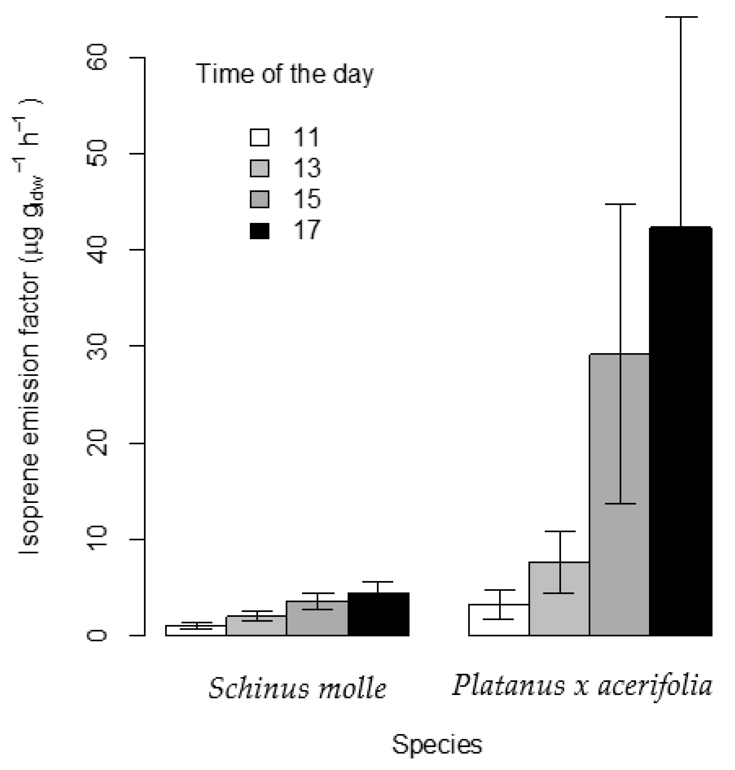
Figure 3 shows the EF of isoprene increasing in the series: 11, 13, 15 and 17 h consistently for both species. The mean normalized EF obtained for Platanus × acerifolia was 20.62 ± 18.41 µg gldw−1 h−1, in good agreement with the 18.5 µg gldw−1 h−1 reported by Scholz (2019) [22] in Sweden and 27 ± 25.3 µg gldw−1 h−1 by Aydin et al. (2014) [23] for Platanus orientalis in Turkey. Jing et al. (2020) reported an EF for Platanus occidentalis of 21.36 µg gldw−1 h−1 in Beijing [24]. Ehsan et al. (2017) [18] obtained average emission values in a wide range from 1.5 to 45 µg gldw−1 h−1 for P. orientalis depending on whether measurements were taken at the beginning or at the end of the season, respectively, in Iran, which may suggest a strong dependence of emissions on the season and variant of Platanus.
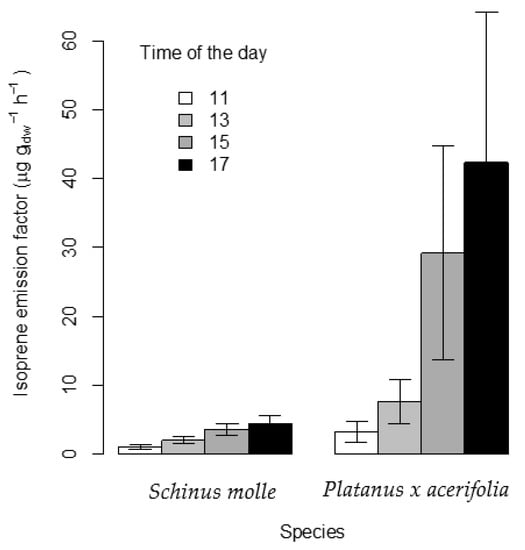
Figure 3.
Standardized emission factor of isoprene (EF) and the corresponding standard error expressed as µg gldw−1 h−1 for Platanus × acerifolia and Schinus molle at different times of the day.
The EF for S. molle, being consistent in trend with those of P. × acerifolia, exhibited consistently lower values, ranging from a minimum of 1.1 ± 0.8 µg gldw−1 h−1 to a maximum of 4.4 ± 2.9 µg gldw−1 h−1. Thus, the mean values of EF in S. molle were 33.2%, 26.1%, 12.35% and 10.35% of those recorded for P. × acerifolia at 11:00, 13:00, 15:00 and 17:00 h, respectively (Figure 3).
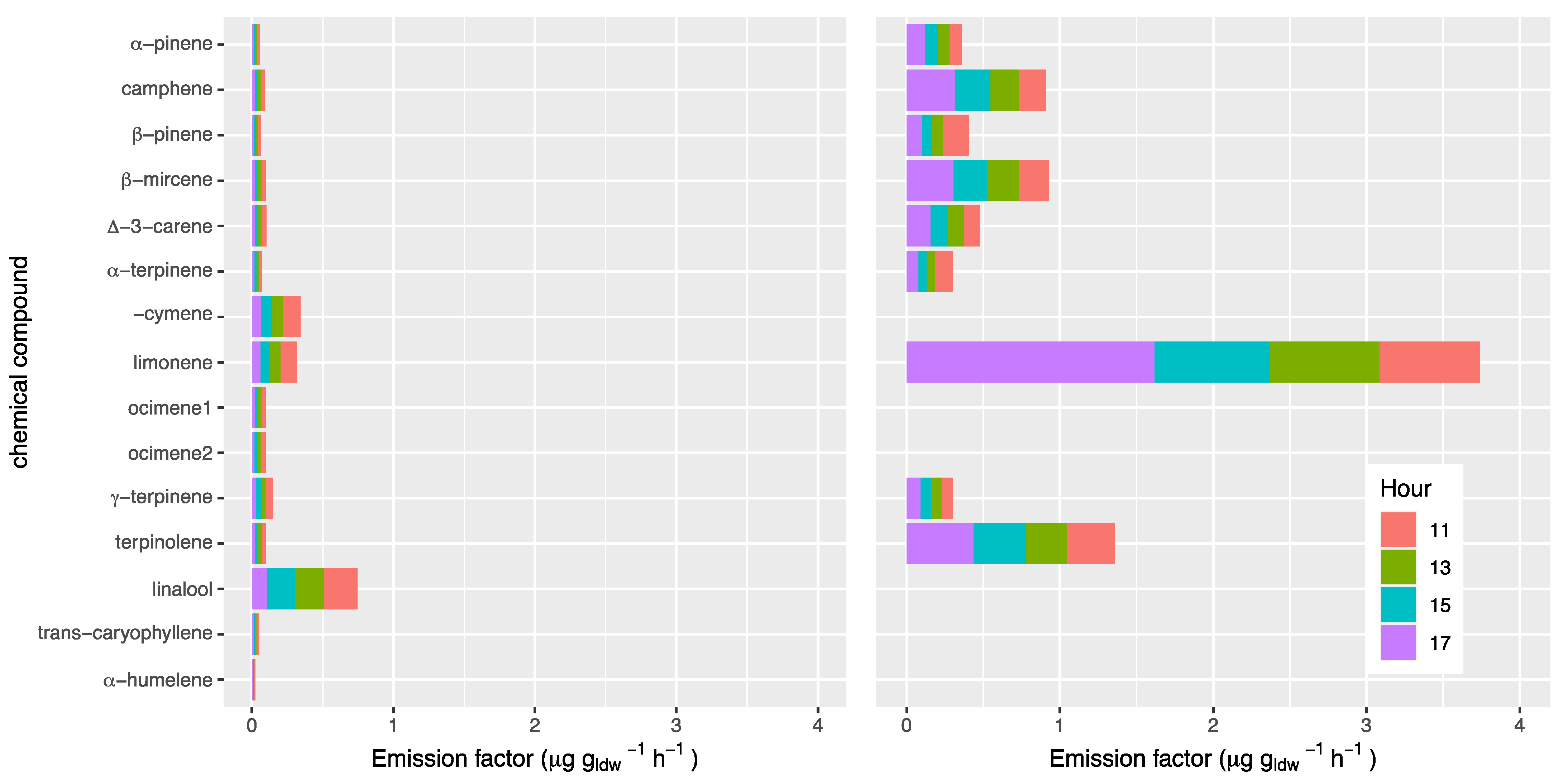
Terpenes other than isoprene contrasted strongly between P. × acerifolia and S. molle. First, P. × acerifolia emitted all 15 terpenes measured other than isoprene while S. molle only emitted nine (Figure 4). Second, emission factors for S. molle were much greater than those of P. × acerifolia for those mono- and sesquiterpenes measured that exhibited any rate of emission for both species. Third, a marked diurnal variation was observed for some compounds also contrasting between species.

Figure 4.
Standardized emission factor, expressed as µg gldw−1 h−1 during the day and standard deviation of monoterpenes, transcaryophillene and alfa-humelene for Platanus × acerifolia (left) and Schinus molle (right).
Twelve monoterpenes and two sesquiterpenes exhibited greater emissions in the morning, decreasing in the afternoon for P. × acerifolia, which was in contrast to the behavior of normalized isoprene (Figure 3). For S. molle, this pattern was also observed for some terpenes other than isoprene. Such pattern differences between isoprene, increasing during the day, and some terpenes other than isoprene, decreasing during the day, are intriguing. We might speculate that isoprene depends mostly on cumulative radiative and temperature stresses, while terpenes other than isoprene on metabolic activity which are higher at 11:00 am, with more favorable environmental conditions which become harsher later during the day. Another explanation could be that the monoterpenes are synthesized and stored to be emitted when required to provide specific metabolic signals, unlike isoprene, which is synthesized and emitted immediately according to radiative and temperature stresses.
The mean EF for total monoterpenes and the two sesquiterpenes for P. × acerifolia was 0.11 ± 0.03 µg gldw−1 h−1. Scholz (2019) [22] reported an EF of total monoterpenes between 0.1 and 3.9 µg gldw−1 h−1 for Platanus × hispanica (or P. × acerifolia). Aydin et al. (2014) [23] reported an EF of total monoterpenes of 0.025 ± 0.006 µg gldw−1 h−1 for P. orientalis. The authors agree on the results for monoterpenes, but not for isoprene in the case of Platanus.
For S. molle, EF of terpenes other than isoprene showed little change throughout the day except for limonene. Monoterpene emissions are known to be variable throughout the day and among days, the season, as well as the age of the individual [22]. However, the 1–8 cineole, followed by β-myrcene and limonene are the species with the highest EF from S. molle according to Préndez et al. (2013a) [25]. The terpene 1–8 cineole was not measured in this study. Limonene exhibited the highest EF of monoterpenes followed by terpinolene.
3.2. Mean and Total EF and Photochemical Ozone Creation Index, POCI
Table 1 shows the mean EF (n = 20) for every analyzed terpene, the total EF considering all terpenes, their respective POCI and the C flux for P. × acerifolia and S. molle. Table S3 shows the transformation procedure from EF to carbon flux of terpenes emitted by Platanus × acerifolia and Schinus molle. The total EF of P. × acerifolia was dominated by isoprene, which makes 99.4% while for POCI isoprene makes about 99.6%. The correlations (Pearson-r) between EF and environmental variables were significant between relative humidity and α-terpinene and α-humulene compounds with r = 0.646 and 0.635, respectively.

Table 1.
Mean emission factor (EF) and standard deviation (SD) of BVOCs, expressed as µg gldw−1 h−1, Photochemical Ozone Creation Index (POCI) and C flux for all quantified terpenes in Platanus × acerifolia and Schinus molle. Total C uptake (photosynthesis) less C released as BVOCs are presented as Net Carbon Flux.
The contribution of isoprene to the total EF of S. molle was 86.3% with a lower amount of monoterpenes, being higher compared to P. × acerifolia. The POCI of S. molle was dominated by isoprene, which makes this compound the main ozone precursor for this species. However, the POCI of S. molle is 6.9 times smaller than the one for P. × acerifolia.
3.3. Methane and CO2 Fluxes
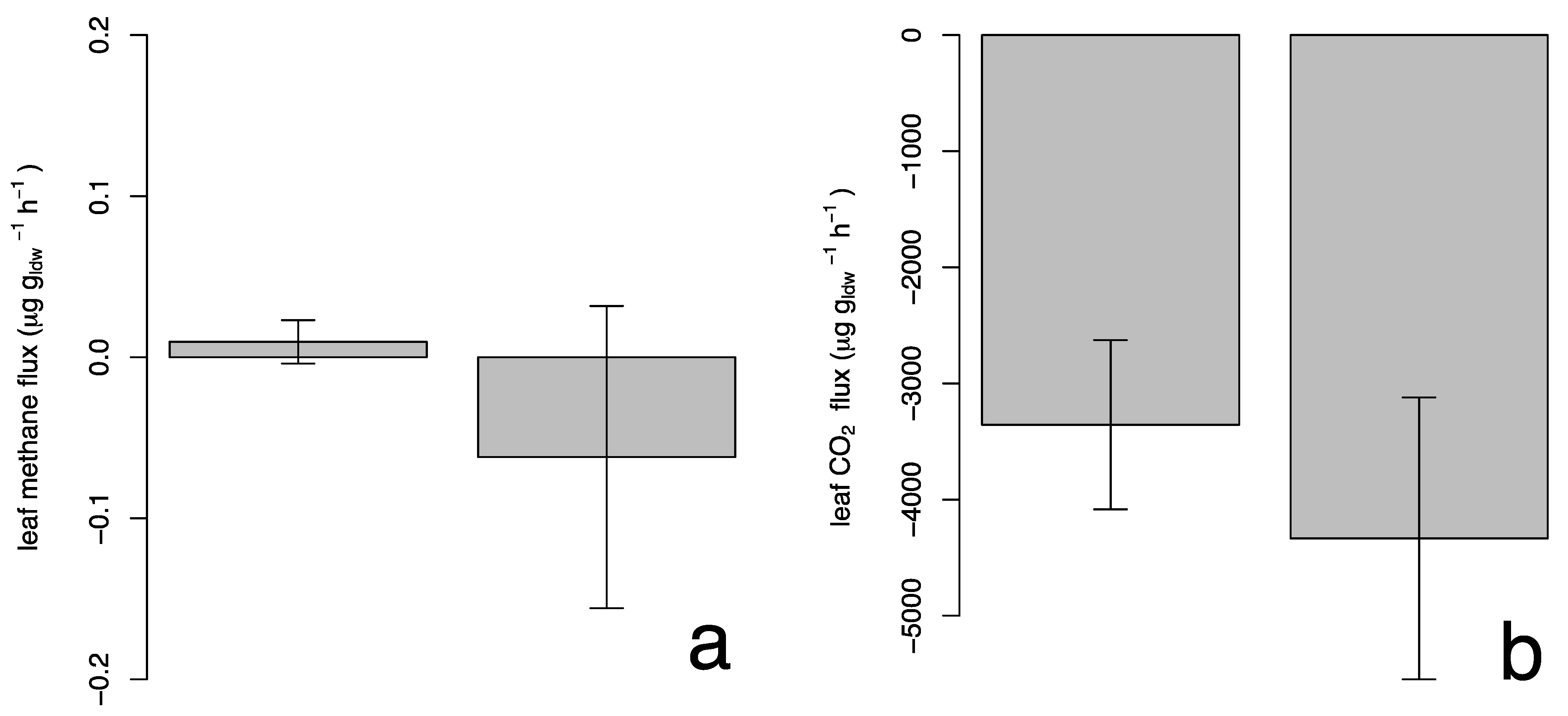
Figure 5a shows the methane flux for the studied species with an average value of 0.0010 ± 0.06 µg gldw−1 h−1 and −0.061 ± 0.41 µg gldw−1 h−1 for P. × acerifolia and S. molle, respectively; where the positive values indicate emission of the compound and the negative values indicate removal. However, a t-Student analysis showed that the methane fluxes were not significantly different from zero, suggesting that plant foliage neither release nor capture methane.

Figure 5.
Leaf methane (a) and photosynthesis (b) fluxes for Platanus × acerifolia and Schinus molle (mean ± 1 standard error).
Different researchers found variable methane emissions in small plants [26,27,28]. In those works, the methane concentration chambers were connected to the ground or very close to it, so the results could include contributions of methane due to its proximity to the soil. On the other hand, in this work, we made the analysis at a 2 m height, so potential contributions from the ground would be reduced, resulting in non-significant flows. Figure 5b shows the total CO2 fluxes due to photosynthesis. The mean CO2 uptake value is −0.0033 ± 0.0032 µg gldw−1 h−1 in P. × acerifolia and −0.0042 ± 0.0055 µg gldw−1 h−1 in S. molle. In both cases, there was found to be a negative mean, which indicates carbon fixation by both species. Photosynthetic rates were 29% higher for S. molle compared to P. × acerifolia, but such difference was insignificant. It is worth noting that P. × acerifolia exhibited a total EF 6.4 times greater than for S. molle, for a similar photosynthetic rate.
For P. × acerifolia, measured BVOCs fluxes represented about 2% of photosynthetic rates while only representing 0.24% for S. molle, for which isoprene is the greatest contributor followed by limonene (Table 1, Figure 4). With P. × acerifolia outside its environmental range, it could be placed under a constant physiological stress that enhances the proportionally its BVOCs emissions compared to carbon fixation over other species particularly native ones [17].
4. Conclusions
Total carbon fixation in S. molle was similar to P. × acerifolia during the hot dry summer sampling days, but BVOC emissions were proportional to photosynthesis at a much greater rate in P. × acerifolia (2%) compared to S. molle (0.24%). Methane emission fluxes were not significantly different from zero for both species and were therefore considered negligible.
The total EF of P. × acerifolia was 20.72 µg gldw−1 h−1, being around 6.4 times greater than the EF of Schinus molle (3.14 µg gldw−1 h−1). For both species, isoprene was the dominant terpene with the contribution to the total EF being 99.4% and 86.3% for P. × acerifolia and S. molle, respectively. Moreover, isoprene emission rates increased throughout the day reaching its maximum at 5:00 p.m.
The highest emission of monoterpenes in P. × acerifolia corresponds to linalool with 0.047 µg gldw−1 h−1 at 11:00, while in S. molle the greater monoterpene emission was limonene with an EF of 0.32 µg gldw−1 h−1 at 5:00 p.m. No significant correlations were found between the environmental variables and the normalized concentrations and/or EF of terpenes except for the terpinolene-temperature relationship in Schinus molle. The total POCI in S. molle was 342 with about 92.1% accounted for by isoprene, while for P. × acerifolia the total POCI was 2359, being 6.9 times higher compared to the former, with an isoprene contribution of 99.6%.
The 6.4 times greater BVOCs emission factor of P. × acerifolia compared to S. molle may suggest that P. × acerifolia, being an exotic species growing outside its ecological range, might have been subject to water, radiative and temperature stresses that triggered such a response. If it is true that stressed plants would exhibit higher BVOCs emission rates, then selecting plant species better adapted to particular environmental conditions may contribute to reducing a tropospheric ozone in highly polluted urban environments. P. × acerifolia is a species that loses its leaves in the autumn-winter period. On the contrary, S. molle is a species with permanent leaves and therefore carries out the fixation process the whole year. These results should be taken into account by the authorities for urban reforestation plans.
We are aware that only one tree of P. × acerifolia and one of S. molle were measured repeatedly over five days and four times daily. This is a limiting factor of the study brought about by the infeasibility to measure more trees. Both trees selected were healthy adult individuals without irrigation during the summer period. Rainfall was the only source of water for these trees. There are uncertainties associated with the lack of replication, although repeated measurements for the same individuals may provide indications of the identification of the main chemical species of BVOCs and magnitude. This study should be considered as exploratory rather than statistically representative of the populations studied.
Supplementary Materials
The following supporting information can be downloaded at: https://www.mdpi.com/article/10.3390/atmos13020298/s1, Table S1: Retention time and main terpene masses; Table S2: Detection (LOD) and quantification (LOQ) limits of the studied terpenes. Table S3 Transformation procedure from emission factor to carbon flux of terpenes emitted by Platanus × acerifolia and Schinus mole.
Author Contributions
Formal analysis, investigation, methodology and software, I.F.; Conceptualization, investigation, resources, writing—original draft preparation, writing—review and editing, supervision, project administration and funding acquisition, M.P.; Conceptualization, investigation, methodology, writing—original draft preparation, funding acquisition and supervision, H.E.B. All authors have read and agreed to the published version of the manuscript.
Funding
This research was funded by Universidad de Chile grant number URC-026/17 and CONICYT grant number FONDECYT 1150877.
Data Availability Statement
Data are available after request to corresponding author.
Acknowledgments
To the REDES consolidation project of the Universidad de Chile URC-026/17 for financial support. This study was also supported by the Chilean Commission of Science and Technology (CONICYT) through Grant FONDECYT Nº 1150877.
Conflicts of Interest
The authors declare no conflict of interest.
References
- Tyrväinen, L.; Pauleit, S.; Seeland, K.; de Vries, S. Benefits and Uses of Urban Forests and Trees. In Urban Forests and Trees; Konijnendijk, C., Nilsson, K., Randrup, T., Schipperijn, J., Eds.; Springer: Berlin/Heidelberg, Germany, 2005; pp. 81–144. [Google Scholar]
- Huang, C.; Chen, C.; Li, L.; Cheng, Z.; Wang, H.; Huang, H.; Cheng, Y.; Streets, D.G.; Wang, Y.J.; Zhang, G.F.; et al. Emission inventory of anthropogenic air pollutants and VOC species in the Yangtze River Delta region, China. Atmos. Chem. Phys. 2011, 11, 4105–4120. [Google Scholar] [CrossRef] [Green Version]
- Loreto, F.; Schnitzler, J.P. Abiotic stresses and induced BVOCs. Trends Plant Sci. 2010, 15, 154–166. [Google Scholar] [CrossRef] [PubMed]
- Seinfeld, J.; Pandis, S. Chemistry of the Troposphere. In Atmospheric Chemistry and Physics: From Air Pollution to Climate Change; Seinfeld, J.H., Pandis, S.N., Eds.; John Wiley & Sons: Hoboken, NJ, USA, 2016; pp. 208–211. [Google Scholar]
- Forester, C.; Wells, J. Hydroxyl radical yields from reactions of terpene mixtures with. Indoor Air 2011, 21, 400–409. [Google Scholar] [CrossRef] [PubMed]
- Jerrett, M.; Burnett, R.; Pope, C.; Ito, K.; Thurston, G.; Krewski, D.; Shi, Y.; Calle, E.; Thun, M. Long-Term Ozone Exposure and Mortality. N. Engl. J. Med. 2009, 360, 1085–1095. [Google Scholar] [CrossRef] [PubMed] [Green Version]
- Jurán, S.; Grace, J.; Urban, O. Temporal Changes in Ozone Concentrations and Their Impact on Vegetation. Atmosphere 2021, 12, 82. [Google Scholar] [CrossRef]
- Pellegrini, E.; Hoshika, Y.; Dusart, N.; Cotrozzi, L.; Gérard, J.; Nali, C.; Vaultier, M.-N.; Jolivet, Y.; Lorenzini, G.; Paoletti, E. Antioxidative responses of three oak species under ozone and water stress conditions. Sci. Total Environ. 2019, 647, 390–399. [Google Scholar] [CrossRef]
- Elshorbany, Y.; Kleffmann, J.; Kurtenbach, R.; Rubio, M.; Lissi, E.; Villena, G.; Gramash, E.; Rickard, A.; Pilling, M.J.; Wiesen, P. Summertime photochemical ozone formation in Santiago, Chile. Atmos. Environ. 2009, 43, 6398–6407. [Google Scholar] [CrossRef]
- Préndez, M.; Araya, M.; Criollo, C.; Egas, C.; Farías, I.; Fuentealba, R.; González, E. Urban trees and its relationships with air pollution by particulate matter and ozone in Santiago de Chile. In Urban Climate in Latin-American Cities; Henríquez, C., Romero, H., Eds.; Springer International Publishing: Cham, Switzerland, 2019; pp. 167–206. [Google Scholar]
- SINCA. Sistema de Información Nacional de Calidad del Aire. Available online: https://sinca.mma.gob.cl/index.php/pagina/index/id/glosario (accessed on 15 July 2015).
- Seguel, R.J.; Gallardo, L.; Fleming, Z.; Landeros, S. Two decades of ozone standard exceedances in Santiago de Chile. Air Qual. Atmos. Health 2020, 13, 593–605. [Google Scholar] [CrossRef]
- Gramsch, E.; López, G.; Gidhagen, L. Estudio “Actualización y Sistematización del Inventario de Emisiones de Contaminantes Atmosféricos en la Región Metropolitana”; Departamento de Física, Universidad de Santiago de Chile: Santiago, Chile, 2014; Available online: https://sustempo.com/website/wp-content/uploads/2015/07/Inventario-deemisiones-RM_USACH_2014.pdf (accessed on 1 January 2022).
- Simon, V.; Dumergues, L.; Solignac, G.; Torres, L. Biogenic emissions from Pinus halepensis: A typical species of the Mediterranean area. Atmos. Res. 2005, 74, 37–48. [Google Scholar] [CrossRef]
- Padhy, P.; Varshney, C. Isoprene emission from tropical tree species. Environ. Pollut. 2005, 135, 101–109. [Google Scholar] [CrossRef]
- Moukhtar, S.; Couret, C.; Rouil, L.; Simon, V. Biogenic Volatile Organic Compounds (BVOCs) emissions from Abies alba in a French forest. Sci. Total Environ. 2006, 354, 232–245. [Google Scholar] [CrossRef] [PubMed]
- Préndez, M.; Carvajal, V.; Corada, K.; Morales, J.; Alarcón, F.; Peralta, H. Biogenic volatile organic compounds from the urban forest of the Metropolitan Region, Chile. Environ. Pollut. 2013, 183, 143–150. [Google Scholar] [CrossRef] [PubMed]
- Ehsan, K.; Anoushirvan, S.; Mohammad, A.; Thomas, S. In situ emission of BVOCs by three urban woody species. Urban For. Urban Green. 2017, 21, 153–157. [Google Scholar]
- Yaman, B.; Aydin, Y.; Koca, H.; Dasdemir, O.; Kara, M.; Altiok, H.; Dumanoglu, Y.; Bayram, A.; Tolunay, D.; Odabasi, M.; et al. Biogenic Volatile Organic Compound (BVOC) Emissions from Various Endemic Tree Species in Turkey. Aerosol Air Qual. Res. 2015, 15, 341–356. [Google Scholar] [CrossRef] [Green Version]
- Guenther, A.; Zimmerman, P.; Harley, P.; Monson, R.; Fall, R. Isoprene and monoterpene emission rate variability: Model evaluations and sensitivity analyses. J. Geophys. Res. Atmos. 1993, 98, 12609–12617. [Google Scholar] [CrossRef] [Green Version]
- Derwent, R.; Jenkin, M.; Passant, N.; Pilling, M. Photochemical ozone creation potentials (POCPs) for different emission sources of organic compounds under European conditions estimated with a Master Chemical Mechanism. Atmos. Environ. 2007, 41, 2570–2579. [Google Scholar] [CrossRef]
- Scholz, L.L.G. Estimation of the Potential BVOC Emissions by the Different Tree Species in Malmö. Bachelor’s Thesis, Lund University, Lund, Sweden, 2019. Series INES. Available online: https://lup.lub.lu.se/student-papers/search/publication/8986300 (accessed on 1 January 2022).
- Aydin, Y.; Yaman, B.; Koca, H.; Dasmedir, O.; Kara, M.; Altiok, H.; Elbir, T. Biogenic volatile organic compoundas (BVOC) emissions from forested areas in Turkey: Determination of specific emission rates for thirty-one tree species. Sci. Total Environ. 2014, 490, 239–253. [Google Scholar] [CrossRef]
- Jing, X.; Lun, X.; Fan, C.; Ma, W. Emission patterns of biogenic volatile organic compounds from dominant forest species in Beijing, China. J. Environ. Sci. 2020, 95, 73–81. [Google Scholar] [CrossRef]
- Préndez, M.; Corada, K.; Morales, J. Emission factors of biogenic volatile organic compounds in various stages of growth present in the urban forest of the Metropolitan Region, Chile. Res. J. Chem. Environ. 2013, 17, 108–116. [Google Scholar]
- Terazawa, K.; Ishizuka, S.; Sakata, T.; Yamada, K.; Takahashi, M. Methane emissions from stems of Fraxinus mandshurica var. japonica trees in a floodplain forest. Soil Biol. Biochem. 2007, 39, 2689–2692. [Google Scholar] [CrossRef]
- Gauci, V.; Gowing, D.; Hornibrook, E.; Davis, J.; Dise, N. Woody stem methane emission in mature wetland alder trees. Atmos. Environ. 2010, 44, 2157–2160. [Google Scholar] [CrossRef] [Green Version]
- Diaz, M.; Bown, H.; Fuentes, J.; Martinez, A. Soils act as sinks or sources of CH4 depending on air-filled porosity in sclerophyllous ecosystems in semiarid central Chile. Appl. Soil Ecol. 2018, 130, 13–20. [Google Scholar] [CrossRef]
Publisher’s Note: MDPI stays neutral with regard to jurisdictional claims in published maps and institutional affiliations. |
© 2022 by the authors. Licensee MDPI, Basel, Switzerland. This article is an open access article distributed under the terms and conditions of the Creative Commons Attribution (CC BY) license (https://creativecommons.org/licenses/by/4.0/).