Article

Surface Layer Drag Coefficient at Different Radius Ranges in Tropical Cyclones

1
Collaborative Innovation Center on Forecast and Evaluation of Meteorological Disasters, Key Laboratory for Aerosol-Cloud-Precipitation of China Meteorological Administration, School of Atmospheric Physics, Nanjing University of Information Science and Technology, Nanjing 210044, China
2
Southern Marine Science and Engineering Guangdong Laboratory (Zhuhai), Zhuhai 519080, China
3
State Key Laboratory of Atmospheric Boundary Layer Physics and Atmospheric Chemistry, Institute of Atmospheric Physics, Chinese Academy of Sciences, Beijing 100029, China
*
Author to whom correspondence should be addressed.
Atmosphere 2022, 13(2), 280; https://doi.org/10.3390/atmos13020280
Submission received: 6 December 2021 / Revised: 25 January 2022 / Accepted: 1 February 2022 / Published: 8 February 2022

Abstract

:
Using dropsonde data and a flux-profile method, this study investigates the drag coefficient ( C d )–wind speed relationship within different radius ranges. The results show a systematic decrease of friction velocity u * from the range of R/RMW > 1.05 to that of R/RMW < 0.95 (R is the radial location of a dropsonde profile, and RMW is the radius of maximum wind), and the reduction is 5~25% for different wind speeds. Further, within the ranges of either R/RMW > 1.05 or R/RMW < 1.05, a clear feature of “roll-off” at about 35 m s−1 can be obtained. However, the roll feature becomes vague in the ranges of R/RMW < 0.95, R/RMW < 0.85, and R/RMW < 0.75, indicating the TC dynamics within and near RMW play a role in affecting the flux-profile relationship. Even more, C d of R < 0.75RMW deviates significantly from the C d of R < 0.85RMW and R < 0.95RMW, while the deviation between R < 0.85RMW and R < 0.95RMW is much smaller. Especially when 10 m winds exceed 40 m s−1, u * of R < 0.75RMW is significantly larger than that of R < 0.85RMW. This phenomenon is also linked to the TC dynamics (e.g., the large radial gradients of winds and the drastic vertical variation of the bulk Richardson number), but the speculation needs to be verified in future study.

1. Introduction

Tropical cyclone (TC) is one of the most devastating weather systems that cause huge losses of lives and properties [1,2,3,4]. Its enormous energy mostly comes from and dissipates near the surface, which is expressed as enthalpy flux and surface drag [5,6], and the theory is well accepted that the intensity development of TC strongly depends on the ratio of the drag coefficient ( C d ) and enthalpy flux transfer coefficient ( C k ) (e.g., [7,8,9,10]).
With field dropsondes observation and the flux-profile method, Powell et al. [11] first found that C d , under strong wind conditions, peaked at a 10-m wind speed of around 38 m s−1. Donelan et al. [12] also found a similar variation pattern with laboratory measurements, only that C d tended to level off rather than decline after it reached the peak value. While, by using ocean current velocity profiles, Jarosz et al. [13] calculated the drag coefficient with a bottom-up method and also found C d first increased, but later when the 10-m wind speed was larger than about 32 m s−1, it declined with wind speed. Bi et al. [14] used offshore tower observation and found C d peaked at 18 m s−1 and decreased afterward, but leveled off when larger than 27 m s−1. Other studies with various methods generally also found the same feature that C d decreased or leveled off with wind speed when it was larger than around 30 m s−1 (e.g., [15,16,17,18,19,20,21,22,23,24]).
The observation of hurricanes by dropsondes has been carried out for several decades and thousands of profiles have been obtained (e.g., [25,26]), which leads to the hope to thoroughly understand the relationship between drag coefficient and wind speed. Nevertheless, Richter et al. [27] concluded from virtual dropsondes of a numerical simulation that, caused by the sensitivity of this method to the regression procedure, the calculation of C d with dropsondes observation and the flux-profile method was accurate to within approximately 50%. Richter et al. [28] further showed that the flux-profile method had an inherent underestimation inclination of C d at hurricane-force winds, which was a result of the uncertainty in the vertical position of the sonde near the surface and the non-monotonic profile of wind speed with height, but these might be mitigated by selecting the regression profile within about 20–150 m. Through virtual dropsondes, Richter et al. [28] also showed that within the radius of maximum wind (RMW), where the traditional Monin-Obukhov similarity theory was not applicable anymore, C d was drastically underestimated. However, this characteristic was not observed in their study with real dropsondes.
Based on the findings of Richter et al. [28], this study takes a further step to understand how the C d –wind speed relationship is within the RMW based on the real dropsondes. Especially, under the same 10-m wind speed, how the C d calculated from the flux-profile method varies with RMW. This paper is organized as follows. Section 2 describes the data and the methods used in this paper. Section 3 presents the results, including the variation of friction velocity ( u * ) against R/RMW in the real dropsonde observations. And this is followed by a summary and conclusions in Section 4.

2. Data and Methods

2.1. Data

Dropsonde data used in this study are from the Long-Term NOAA Dropsonde Hurricane Archive released by NOAA’s National Hurricane Center and Hurricane Research Division (https://data.eol.ucar.edu/dataset/542.001 (accessed on 5 December 2021)). The data in this archive include over 13,600 Global Positioning System (GPS) dropsonde profiles from 120 TCs in the Atlantic and East Pacific basins from 1996 to 2012 [26]. The GPS dropsondes are released from aircrafts flying into the TC system, and aircraft types include P3 (flying at 1–5 km altitude in the inner and outer core of TC) and G-IV (flying at 14–15 km altitude in the outside environment of TC). The data quality control of the sounding data is processed by Atmospheric Sounding Processing Environment (ASPEN) software, and various visualization tools and statistical methods are used to evaluate data products to identify and correct data quality problems caused by various errors and deviations. The wind speed is observed at 4 Hz frequency, corresponding to 3–8 m vertical resolution, but prior to 2010, the frequency of wind data was measured at 2 Hz. More detailed information about the dataset can be found in the data archive and Wang et al. [26].
In this work, the radial locations of the profiles (R) are also given by the Dropsonde Hurricane Archive introduced above, while the RMW data are from the Extended Best Track (EBT) dataset [29], which includes 6-h interval RMW data of the corresponding TCs in the Dropsonde Hurricane Archive. The EBT RMW data are then interpolated linearly to fit the R data of the dropsonde profiles.

2.2. Method

Following Powell et al. [11], Holthuijsen et al. [16], and Richter et al. [27], we use the flux-profile method to estimate the drag coefficient C d , which is based on the logarithmic profile of wind speed within the hurricane boundary layer. According to Monin-Obukhov (MO) similarity theory, the wind profile in the neutral condition can be described as
U = u * k ln ( z z 0 ) ,
l n z = ( k u * ) U + l n z 0 ,
where U is the wind speed at altitude z and the Von Karman constant k is taken as 0.4. The friction velocity u * and the roughness length z 0 can be estimated through logarithmic linear regression. Then C d can be derived from
τ = ρ u * 2 = ρ C d U 10 2 ,
where U 10 is the 10-m wind speed and ρ is air density.
Following the approach used in Powell et al. [11] and Richter et al. [28], the vertical profiles of wind speed are analyzed in a composite sense, as a function of the mean boundary layer (MBL, here defined as the height of 10 to 500 m) wind speed. That is, the dropsonde profiles are grouped by their MBL mean wind speeds. This study considers only dropsonde profiles with MBL wind speed larger than 20 m s−1, and 3661 dropsonde profiles meet this criterion. Figure 1 presents the number of profiles in each 5 m s−1 MBL mean wind speed bin, which shows a decreasing trend with increasing wind speed. The data are also categorized by R/RMW to analyze the C d –wind speed relationship at different R/RMW ranges. Figure 1 also presents the number of profiles in the ranges of R > 1.05RMW, R < 1.05RMW, and R < 0.75RMW. Here, the value of 1.05 of R/RMW is chosen to divide the profiles within and outside of the RMW, while the selection of 0.75 of R/RMW as a dividing point is determined by the fact that in the range of R < 0.75RMW there are still relatively large quantity observations. It also can be seen from Figure 1 that the sample numbers are less in high wind speed 5 m s−1 bins, and to maintain a relatively large quantity of samples in each MBL mean wind speed group, the wind speed intervals are chosen as 20–25 m s−1, 25–30 m s−1, 30–35 m s−1, 35–40 m s−1, 40–45 m s−1, 45–50 m s−1, 50–60 m s−1, 60–70 m s−1, and 70–90 m s−1 as in Table 1. Richter et al. [28] used both real and virtual dropsondes to examine the flux-profile method, and they found an underestimation of C d through the flux-profile method with virtual dropsondes, but not with real dropsondes. By using the virtual dropsondes from a full physics simulation, a large number of profiles can be obtained, and Richter et al. [28] divided these virtual samples by an interval of 0.26RMW (Figures 10 and 11 in Richter et al. [28]). However, for the real dropsondes, they used an interval of 1 RMW due to the limited samples (Figure 3 in Richter et al. [28]). Here, we follow Richter et al. [28] using 1.05RMW as a watershed, and 0.75RMW as the lowest limit to guarantee relatively enough samples (more than ~30 for each 10 m s−1 bin), and between 1.05RMW to 0.75RMW we use an interval of 0.05RMW to see how the flux-profile relationship varied from 0.75 to 1.05 RMW (Table 1).
Next, each measurement in each profile is further binned into 10-m height intervals, and the measurements within each height bin are collected and averaged together. Variability associated with mesoscale, convective, and under-sampled turbulent scales is then removed by averaging all profiles in a given wind speed group [11,30]. Finally, we choose the 20 to 160 m height range over which the fit to the mean profiles will be made, based on the suggestion of Powell [31] that 20–160 m surface layer is more representative for the lowest levels. Meanwhile, Richter et al. [28] and Jiang et al. [32] also indicated that under 20 m height, the vertical position of dropsondes might be contaminated; besides, the regressed C d began to decrease monotonically once the upper height bound exceeded roughly 150 m. Byrne and Zhang [33] found that there was a transition of the flow from 3-D to 2-D turbulence in the hurricane boundary layer occurring around 150 m, suggesting that above 150 m MO similarity theory does not apply.
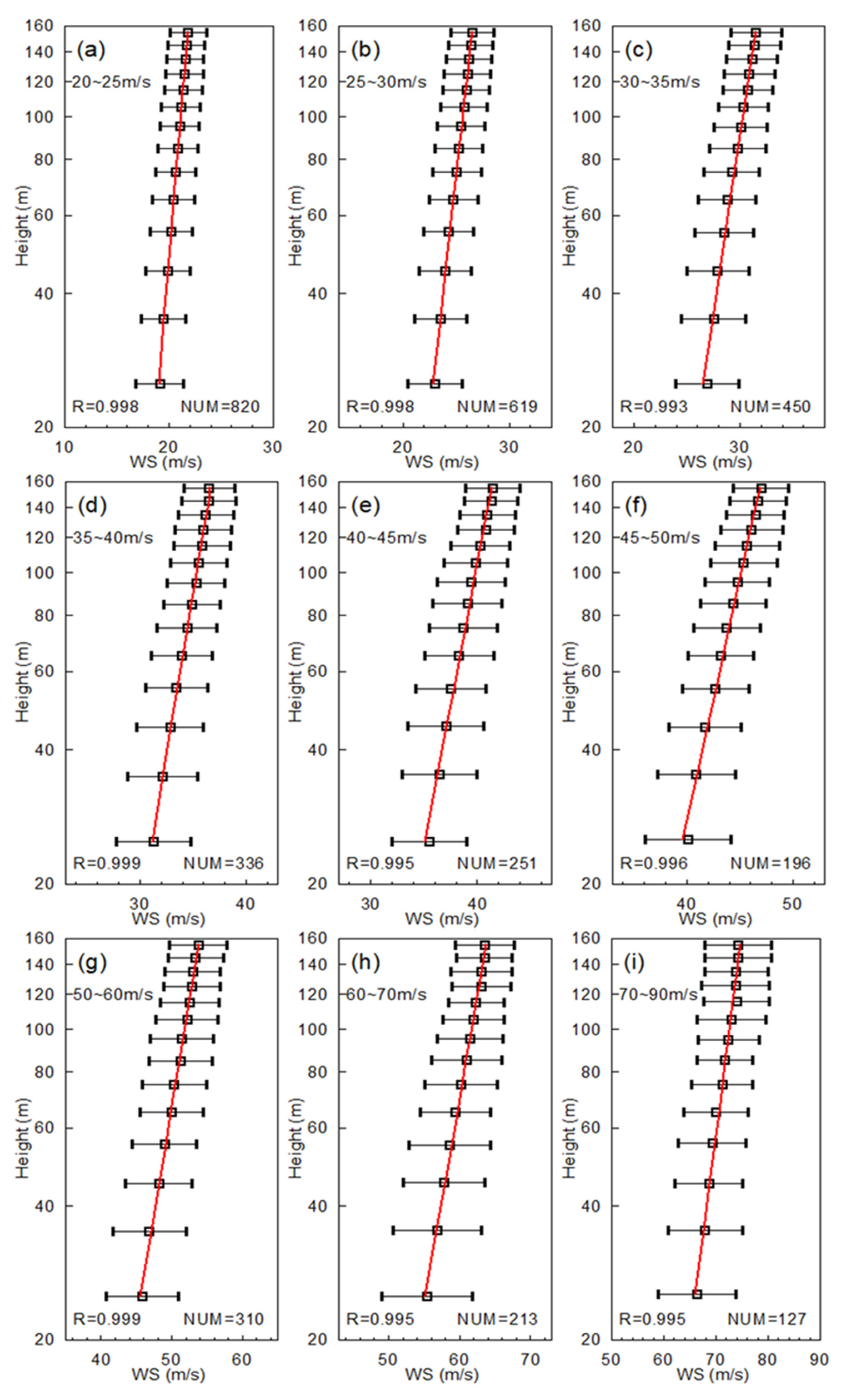
The 20–160 m of each MBL mean wind speed group are plotted in Figure 2 with a semi-log coordinate, and a least-squares linear regression fit is used to estimate the roughness length z 0 (as intercept), friction velocity u * ( k / u * as slope), and 10-m wind speed U 10 , then drag coefficient C d was computed from Equation (3). It can be seen that the regression coefficient of each group is above 99%, indicating the sample size of each MBL mean wind speed group is large enough, and this guarantees the validity of the fitting results.

3. Results

Figure 3 depicts the u * obtained in this study, but within different R/RMW ranges, and also the u * derived by previous studies. It can be found that the u * obtained from the various studies generally shows the same increasing trend when the 10-m wind speed is less than 40 m s−1, but levels off (or presents a smaller increasing trend) at higher wind speeds. Specifically, the data points obtained from the range of R/RMW > 1.05 and R/RMW < 1.05 bear very little difference, except that only at the 10-m wind speed of about 38 m s−1 does the R/RMW < 1.05 group show an evidently smaller value of u * than the R/RMW > 1.05 group, which is even smaller in the group of R/RMW < 0.75. By using virtual dropsondes, Richter et al. [28] showed that with a decreasing R/RMW, the u * obtained by the flux-profile method tends to be underestimated (Figures 10 and 11 in Richter et al. [28]), which are seen here in the 10-m wind speed of about 38 m s−1. At other wind speed ranges, either no significant difference is observed (e.g., at a 10-m wind speed range of 40–50 m s−1), or the results from the group of R/RMW < 0.75 are even larger than from the group of R/RMW > 1.05 (e.g., at a 10-m wind speed ranges of 50–70 m s−1).
Richter et al. [28] also draw a similar conclusion that the different R/RMW ranges generally do not affect the C d –10-m wind speed relationship (Figure 3), which is a result of the various profiles from many TCs with different sizes and intensities.
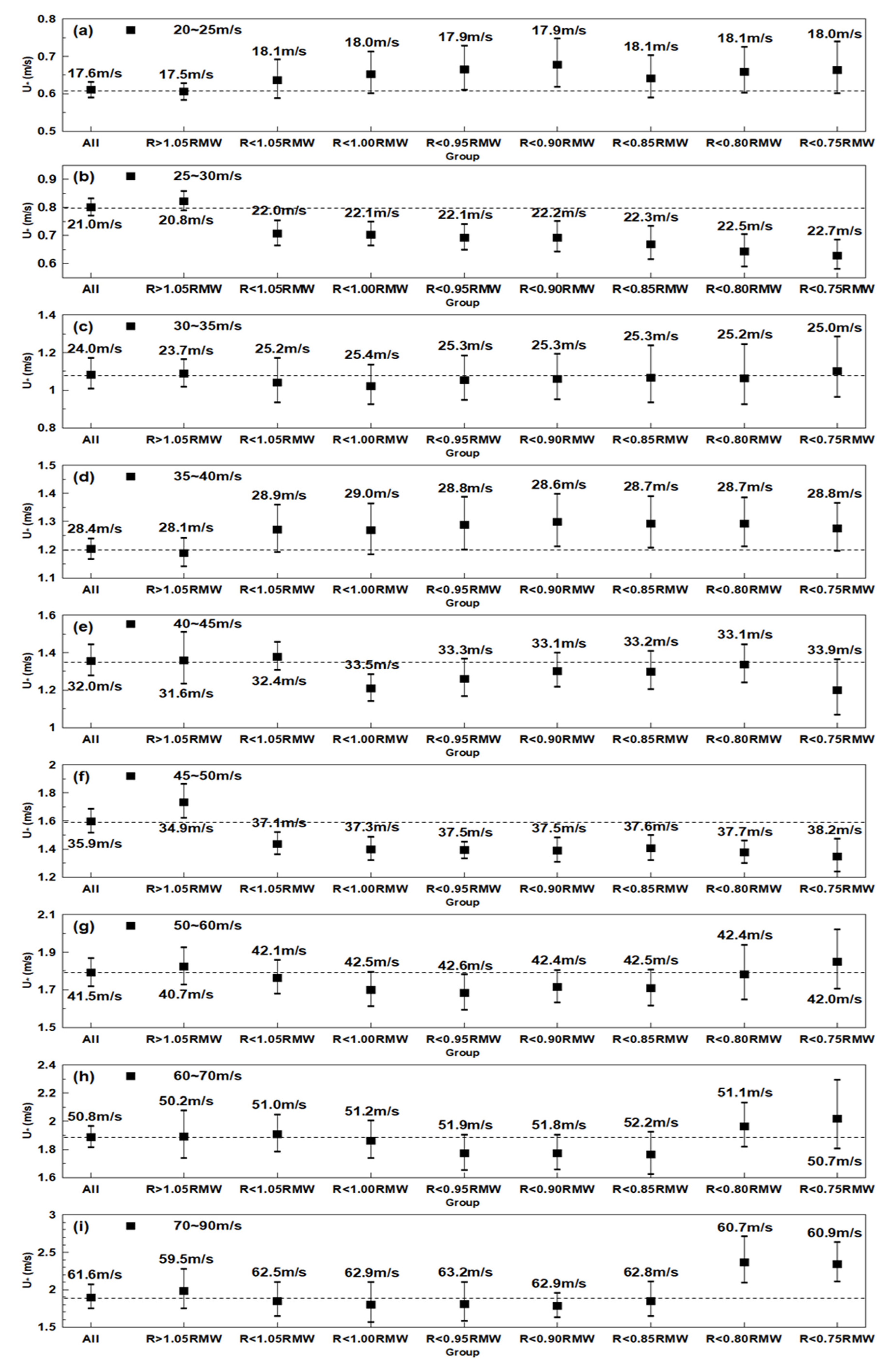
To further look into the u * U 10 relationship under different R/RMW conditions, we plot the variation of u * with R/RMW in the range of >1.05, <1.05, and later on at 0.05 interval to <0.75 (Figure 4). When comparing the u * in the ranges of R/RMW > 1.05 and <0.95, a systematic decrease of u * with R/RMW is generally found for all MBL mean wind speed groups, except the 20–25 m s−1 and 35–40 m s−1 MBL mean wind speed groups. Richter et al. [28] showed by virtual dropsondes, that with a U 10 of about 65 m s−1 and R/RMW of about 0.85 (and U 10 of about 40 m s−1 and R/RMW of about 0.7), u * was underestimated by about 10~20% percent (Figure 10c,d in Richter et al. [28]). Here, although the real dropsondes do not repeat these values exactly, a reduction of u * by 5~25% from R/RMW > 1.05 to <0.95 is observed in the 7 out of 9 MBL mean wind speed groups.
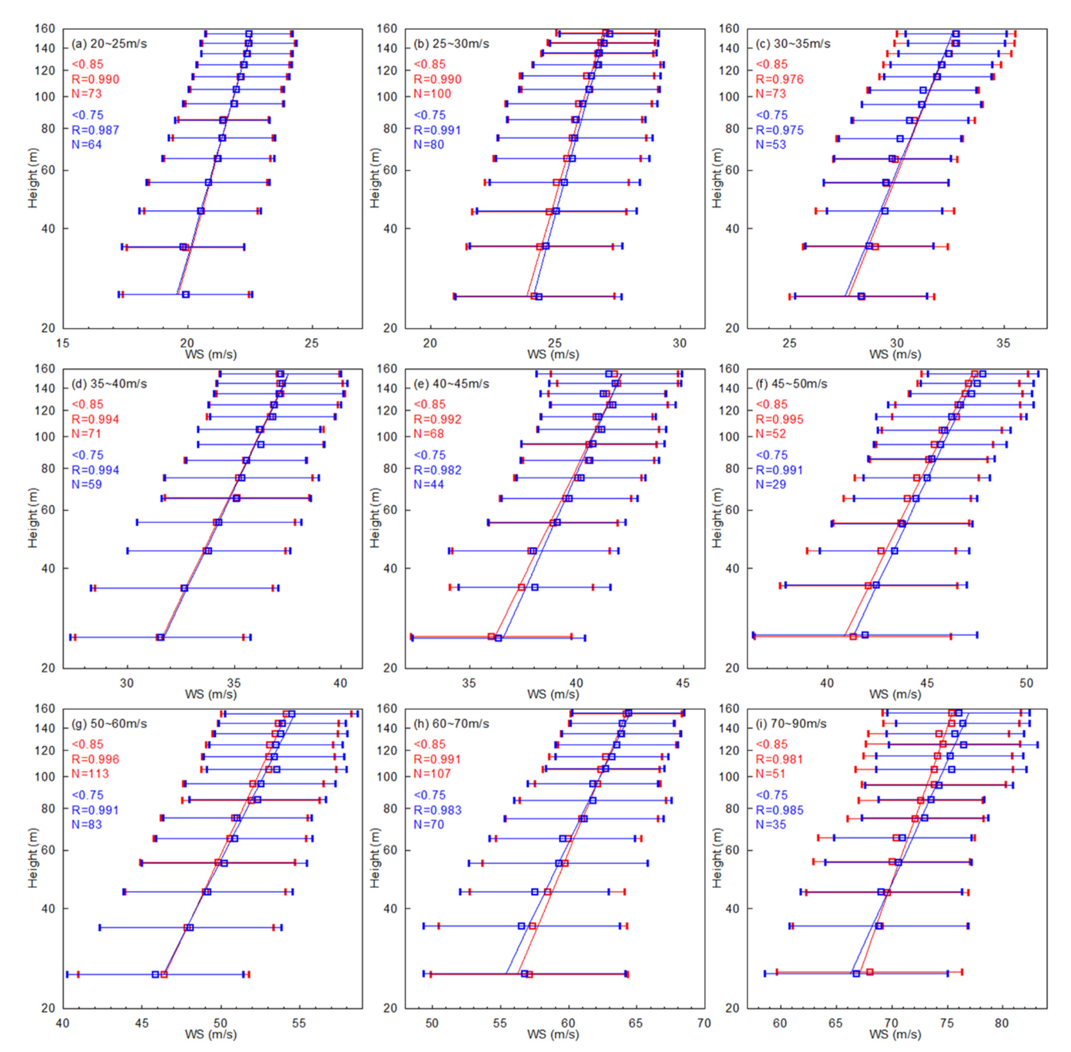
Nonetheless, an unexpected increase of u * with R/RMW from R/RMW < 0.85 to <0.75 is found in the groups of an MBL mean wind speed larger than 50 m s−1. This contradicts the findings of Richter et al. [28]. To examine whether this is caused by some extreme values that could bias the mean of the distribution when sample sizes are small, the wind profiles of R < 0.85RMW and R < 0.75RMW in all MBL mean wind speed groups are presented here as Figure 5. It can be found that for all the wind profiles, a logarithmic profile is generally kept, but when the mean MBL mean wind speed is larger than 50 m s−1, an increase of u * (i.e., decrease of the slope of the profile) is found from R < 0.85RMW to R < 0.75RMW. This phenomenon may be caused by the drastic radial gradient of winds and temperature inside the RMW, as shown in previous studies (e.g., Kepert and Wang [34]; Bell and Montgomery [35]; Zhang et al. [36]). Zhang et al. [36] also found that the depth of the non-strongly stable layer (i.e., the layer with a bulk Richardson number < 0.25) decreased significantly from ~700 m at the RMW to ~200 m at 0.5 RMW (Figure 9 in Zhang et al. [36]), which is less than half of our 500 m MBL layer depth. A bulk Richardson number is an important parameter to indicate the turbulent mixing intensity, and in the atmospheric models, 0.25 is usually used as the marker of the boundary layer height. Combining these findings, it is speculated that when it comes to about < 0.75RMW, the logarithmic wind profile is affected by the TC dynamics (e.g., the large radial gradients of winds and the drastic vertical variation of the bulk Richardson number). This phenomenon will be further investigated in the future through a high-resolution simulation study.
Figure 6 shows the C d –10-m wind speed relationship under different R/RMW ranges. Generally, when considering all the data or the data with R/RMW > 1.05, a clear feature of “roll-off” at about 35 m s−1 can be obtained. Even, if considering the whole range of R/RMW < 1.05, such a feature may still roughly exist. However, at the ranges of R/RMW < 0.95, R/RMW < 0.85, or R/RMW < 0.75, the roll feature becomes vague, indicating the TC dynamics within and near the RMW play a role in affecting the flux-profile relationship. On one hand, the drift of dropsondes with the tangential and radial winds may play a role. Real dropsondes are advected with the horizontal wind, and, in the region near the RMW, that advection can move the sondes 10–20 km downwind as the sondes descend to the surface, violating the flux-profile assumptions. Richter et al. [28] concluded that the effects of a dropsonde drift were negligible, and the features of C d U 10 relationship with and without drift effects were similar to each other. Nevertheless, some differences are still seen in the C d U 10 with and without drift effects, especially, the C d U 10 at 0.78 < R/RMW ≤ 1.04 is significantly different: with/without drift effect, C d is about 0.0018/0.0012, and U 10 is about 65/52 m s−1 (Figures 10 and 11 in Richter et al. [28]). Therefore, the drift of dropsondes within and near RMW indeed plays a role in the C d U 10 relationship. On the other hand, the assumption of the constant flux layer may not be valid anymore within and near the RMW, as pointed by Richter et al. [28], even though a logarithmic layer is persistent throughout all the different ranges of R/RMW. The violation of the constant flux layer may be caused by the large radial gradient of winds and the transport of the momentum flux (e.g., Kepert [37]; Zhang et al., [38]; Bryan et al., [39]).
In addition, in Figure 6b, the C d of R < 0.75RMW (i.e., green square) deviates significantly from the C d of R < 0.85RMW and R < 0.95RMW (i.e., brown and pink squares), while the deviation between R < 0.85RMW (brown squares) and R < 0.95RMW (pink squares) is much smaller, especially when 10 m winds exceed 40 m s−1. As discussed previously, when it comes to about < 0.75RMW, the logarithmic wind profile may be altered by the drift, the large radial gradients, and the advection of the momentum flux here.

4. Summary and Conclusions

Using dropsonde data and flux-profile method, in this study, we investigated the C d –wind speed relationship within different R/RMW ranges, and also the variation of C d with R/RMW under the same wind speed bins. The main findings and conclusions are as follows:
(1)
From the range of R/RMW > 1.05 to that of R/RMW < 0.95, a systematic decrease of 5~25% in friction velocity u * is found for 7 out of the 9 MBL mean wind speed groups.
(2)
A clear feature of “roll-off” at about 35 m s−1 can be obtained for the ranges of either R/RMW > 1.05 or R/RMW < 1.05. However, in the ranges of R/RMW < 0.95, R/RMW < 0.85, and R/RMW < 0.75, the roll feature becomes vague, indicating the TC dynamics within and near the RMW play a role in affecting the flux-profile relationship.
(3)
When U 10 exceeds 40 m s−1, u * of R < 0.75RMW is significantly larger than that of R < 0.85RMW. This phenomenon is not caused by the extreme values in the relatively small sample size, and it is speculated to link with the TC dynamics (e.g., the large radial gradients of winds and the drastic vertical variation of the bulk Richardson number).
At last, these results may be affected by the limited data quantity in this study, and future work will be carried out with more observations and simulations to further understand how the TC dynamics within and near the RMW affect the wind profiles in TCs.

Author Contributions

Conceptualization, Y.L.; methodology, L.Y. and Y.L.; software, L.Y.; validation, L.Y.; formal analysis, L.Y. and Y.L.; investigation, L.Y. and Y.L.; resources, L.Y.; data curation, L.Y.; writing—original draft preparation, L.Y.; writing—review and editing, L.Y., Y.L. and Z.G.; visualization, L.Y.; supervision, Y.L. and Z.G.; project administration, Y.L. and Z.G.; funding acquisition, Y.L. and Z.G. All authors have read and agreed to the published version of the manuscript.

Funding

This study was supported by the National Key Projects of the Ministry of Science and Technology of China (2018YFC1506405); National Natural Science Foundation of China (42075072, 41675009, 41475014); The Innovation Group Project of Southern Marine Science and Engineering Guangdong Laboratory (Zhuhai) (311021008).

Institutional Review Board Statement

Not applicable.

Informed Consent Statement

Not applicable.

Data Availability Statement

Not applicable.

Acknowledgments

The authors thank the three anonymous reviewers for their constructive comments. The numerical calculations in this paper have been done on the supercomputing system in the Supercomputing Center of Nanjing University of Information Science & technology.

Conflicts of Interest

The authors declare no conflict of interest.

References

  1. Pielke, R.A., Jr.; Gratz, J.; Landsea, C.W.; Collins, D.; Saunders, M.A.; Musulin, R. Normalized hurricane damage in the United States: 1900–2005. Nat. Hazards Rev. 2008, 9, 29–42. [Google Scholar] [CrossRef]
  2. Schmidt, S.; Kemfert, C.; Höppe, P. The impact of socio-economics and climate change on tropical cyclone losses in the USA. Reg. Environ. Chang. 2010, 10, 13–26. [Google Scholar] [CrossRef] [Green Version]
  3. Wang, Y.; Wen, S.; Li, X.; Thomas, F.; Su, B.; Wang, R.; Jiang, T. Spatiotemporal distributions of influential tropical cyclones and associated economic losses in China in 1984–2015. Nat. Hazards 2016, 84, 2009–2030. [Google Scholar] [CrossRef]
  4. Wang, H.; Xu, M.; Onyejuruwa, A.; Wang, Y.; Wen, S.; Gao, A.E.; Li, Y. Tropical cyclone damages in Mainland China over 2005–2016: Losses analysis and implications. Environ. Dev. Sustain. 2019, 21, 3077–3092. [Google Scholar] [CrossRef]
  5. Zhang, J.A. Estimation of dissipative heating using low-level in situ aircraft observations in the hurricane boundary layer. J. Atmos. Sci. 2010, 67, 1853–1862. [Google Scholar] [CrossRef] [Green Version]
  6. Heng, J.; Wang, Y. Nonlinear response of a tropical cyclone vortex to prescribed eyewall heating with and without surface friction in TCM4: Implications for tropical cyclone intensification. J. Atmos. Sci. 2016, 73, 1315–1333. [Google Scholar] [CrossRef]
  7. Emanuel, K.A. Sensitivity of tropical cyclones to surface exchange coefficients and a revised steady-state model incorporating eye dynamics. J. Atmos. Sci. 1995, 52, 3969–3976. [Google Scholar] [CrossRef] [Green Version]
  8. Emanuel, K.A. Self-stratification of tropical cyclone outflow. Part II: Implications for storm intensification. J. Atmos. Sci. 2012, 69, 988–996. [Google Scholar] [CrossRef] [Green Version]
  9. Rogers, R.; Aberson, S.; Aksoy, A.; Annane, B.; Black, M.; Cione, J.; Dorst, N.; Dunion, J.; Gamache, J.; Goldenberg, S.; et al. NOAA’S Hurricane Intensity Forecasting Experiment: A Progress Report. Bull. Amer. Meteor. Soc. 2013, 94, 859–882. [Google Scholar] [CrossRef] [Green Version]
  10. Soloviev, A.V.; Lukas, R.; Donelan, M.A.; Haus, B.K.; Ginis, I. The air-sea interface and surface stress under tropical cyclones. Sci. Rep. 2014, 4, 5306. [Google Scholar] [CrossRef]
  11. Powell, M.D.; Vickery, P.J.; Reinhold, T.A. Reduced drag coefficient for high wind speeds in tropical cyclones. Nature 2003, 422, 279–283. [Google Scholar] [CrossRef] [PubMed]
  12. Donelan, M.A.; Haus, B.K.; Reul, N.; Plant, W.J.; Stiassnie, M.; Graber, H.C.; Brown, O.B.; Saltzman, E.S. On the limiting aerodynamic roughness of the ocean in very strong winds. Geophys. Res. Lett. 2004, 31, L18306. [Google Scholar] [CrossRef] [Green Version]
  13. Jarosz, E.; Mitchell, D.A.; Wang, D.W.; Teague, W.J. Bottom-up determination of air-sea momentum exchange under a major tropical cyclone. Science 2007, 315, 1707–1709. [Google Scholar] [CrossRef] [PubMed] [Green Version]
  14. Bi, X.; Gao, Z.; Liu, Y.; Liu, F.; Song, Q.; Huang, J.; Huang, H.; Mao, W.; Liu, C. Observed drag coefficients in high winds in the near offshore of the South China Sea. J. Geophys. Res. Atmos. 2015, 120, 6444–6459. [Google Scholar] [CrossRef]
  15. Sanford, T.B.; Price, J.F.; Girton, J.B. Upper-ocean response to Hurricane Frances (2004) observed by profiling EM-APEX floats. J. Phys. Oceanogr. 2011, 41, 1041–1056. [Google Scholar] [CrossRef]
  16. Holthuijsen, L.H.; Powell, M.D.; Pietrzak, J.D. Wind and waves in extreme hurricanes. J. Geophys. Res. 2012, 117, C09003. [Google Scholar] [CrossRef] [Green Version]
  17. Takagaki, N.; Komori, S.; Suzuki, N.; Iwano, K.; Kuramoto, T.; Shimada, S.; Kurose, R.; Takahashi, K. Strong correlation between the drag coefficient and the shape of the wind sea spectrum over a broad range of wind speeds. Geophys. Res. Lett. 2012, 39, L23604. [Google Scholar] [CrossRef] [Green Version]
  18. Potter, H.; Graber, H.C.; Williams, N.J.; Collins, C.O.; Ramos, R.J.; Drennan, W.M. In situ measurements of momentum fluxes in typhoons. J. Atmos. Sci. 2015, 72, 104–118. [Google Scholar] [CrossRef]
  19. Komori, S.; Iwano, K.; Takagaki, N.; Onishi, R.; Kurose, R.; Takahashi, K.; Suzuki, N. Laboratory measurements of heat transfer and drag coefficients at extremely high wind speeds. J. Phys. Oceanogr. 2018, 48, 959–974. [Google Scholar] [CrossRef]
  20. Hsu, J.Y.; Lien, R.C.; D’Asaro, E.A.; Sanford, T.B. Scaling of drag coefficients under five tropical cyclones. Geophys. Res. Lett. 2019, 46, 3349–3358. [Google Scholar] [CrossRef]
  21. Peng, W.; GAO, Z.; Li, Y.; Zhang, R.; Tong, B.; Wu, B.; He, Y. Testing drag coefficient approaches by using the buoy data collected in moderate to high wind under following, crossing and opposing swell conditions. J. Trop Meteor. 2019, 25, 336–343. [Google Scholar] [CrossRef]
  22. Gao, Z.; Peng, W.; Gao, C.Y.; Li, Y. Parabolic dependence of the drag coefficient on wind speed from aircraft eddy-covariance measurements over the tropical Eastern Pacific. Sci. Rep. 2020, 10, 1805. [Google Scholar] [CrossRef] [PubMed]
  23. Troitskaya, Y.I.; Sergeev, D.A.; Vdovin, M.; Kandaurov, A.; Ermakova, O.; Takagaki, N. Alaboratory study of the effect of surface waves on heat and momentum transfer at high wind speeds. J. Geophys. Res. Oceans 2020, 125, e2020JC016276. [Google Scholar] [CrossRef]
  24. Gao, Z.; Zhou, S.; Zhang, J.; Zeng, Z.; Bi, X. Parameterization of Sea Surface Drag Coefficient for All Wind Regimes Using 11 Aircraft Eddy-Covariance Measurement Databases. Atmosphere 2021, 12, 1485. [Google Scholar] [CrossRef]
  25. Aberson, S.D.; Franklin, J.L. Impact on hurricane track and intensity forecasts of GPS dropwindsonde observations from the first-season flights of the NOAA Gulfstream-IV jet aircraft. Bull. Amer. Meteor. Soc. 1999, 80, 421–428. [Google Scholar] [CrossRef] [Green Version]
  26. Wang, J.; Young, K.; Hock, T.; Lauritsen, D.; Behringer, D.; Black, M.; Black, P.G.; Franklin, J.; Halverson, J.; Molinari, J.; et al. A Long-Term, High-Quality, High-Vertical-Resolution GPS Dropsonde Dataset for Hurricane and Other Studies. Bull. Amer. Meteor. Soc. 2015, 96, 961–973. [Google Scholar] [CrossRef] [Green Version]
  27. Richter, D.H.; Bohac, R.; Stern, D.P. An assessment of the flux profile method for determining air-sea momentum and enthalpy fluxes from dropsonde data in tropical cyclones. J. Atmos. Sci. 2016, 73, 2665–2682. [Google Scholar] [CrossRef]
  28. Richter, D.H.; Wainwright, C.; Stern, D.P.; Bryan, G.H.; Chavas, D. Potential Low Bias in High-Wind Drag Coefficient Inferred from Dropsonde Data in Hurricanes. J. Atmos. Sci. 2021, 78, 2339–2352. [Google Scholar] [CrossRef]
  29. Demuth, J.; DeMaria, M.; Knaff, J.A. Improvement of Advanced Microwave Sounding Unit tropical cyclone intensity and size estimation algorithms. J.J. Appl. Meteor.Meteor. Climatol. 2006, 45, 1573–1581. [Google Scholar] [CrossRef]
  30. Vickery, P.J.; Wadhera, D.; Powell, M.D.; Chen, Y. A hurricane boundary layer and wind field model for use in engineering applications. J.J. Appl. Meteor.Meteor. Climatol. 2009, 48, 381–405. [Google Scholar] [CrossRef]
  31. Powell, M.D. Final Report on the NOAA Joint Hurricane Testbed: Drag Coefficient Distribution and Wind Speed Dependence in Tropical Cyclones; NOAA/AOML: Miami, FL, USA, 2007. [Google Scholar]
  32. Jiang, W.; Wu, L.; Liu, Q. High-Wind Drag Coefficient Based on the Tropical Cyclone Simulated With the WRF-LES Framework. Front. Earth Sci. 2021, 9, 694314. [Google Scholar] [CrossRef]
  33. Byrne, D.; Zhang, J.A. Height-dependent transition from 3-D to 2-D turbulence in the hurricane boundary layer. Geophys. Res. Lett. 2013, 40, 1439–1442. [Google Scholar] [CrossRef]
  34. Kepert, J.; Wang, Y. The Dynamics of Boundary Layer Jets within the Tropical Cyclone Core. Part II: Nonlinear Enhancement. J. Atmos. Sci. 2001, 58, 2485–2501. [Google Scholar] [CrossRef]
  35. Bell, M.M.; Montgomery, M.T. Observed Structure, Evolution, and Potential Intensity of Category 5 Hurricane Isabel (2003) from 12 to 14 September. Mon. Wea. Rev. 2008, 136, 2023–2046. [Google Scholar] [CrossRef] [Green Version]
  36. Zhang, J.A.; Rogers, R.F.; Nolan, D.S.; Marks, F.D. On the Characteristic Height Scales of the Hurricane Boundary Layer. Mon. Wea. Rev. 2011, 139, 2523–2535. [Google Scholar] [CrossRef]
  37. Kepert, J.D. The dynamics of boundary layer jets within the tropical cyclone core. Part I: Linear theory. J. Atmos. Sci. 2001, 58, 2469–2484. [Google Scholar] [CrossRef] [Green Version]
  38. Zhang, J.A.; Drennan, W.M.; Black, P.G.; French, J.R. Turbulence Structure of the Hurricane Boundary Layer between the Outer Rainbands. J. Atmos. Sci. 2009, 66, 2455–2467. [Google Scholar] [CrossRef]
  39. Bryan, G.H.; Worsnop, R.P.; Lundquist, J.K.; Zhang, J.A. A simple method for simulating wind profiles in the boundary layer of tropical cyclones. Boundary-Layer Meteorl. 2017, 162, 475–502. [Google Scholar] [CrossRef] [Green Version]
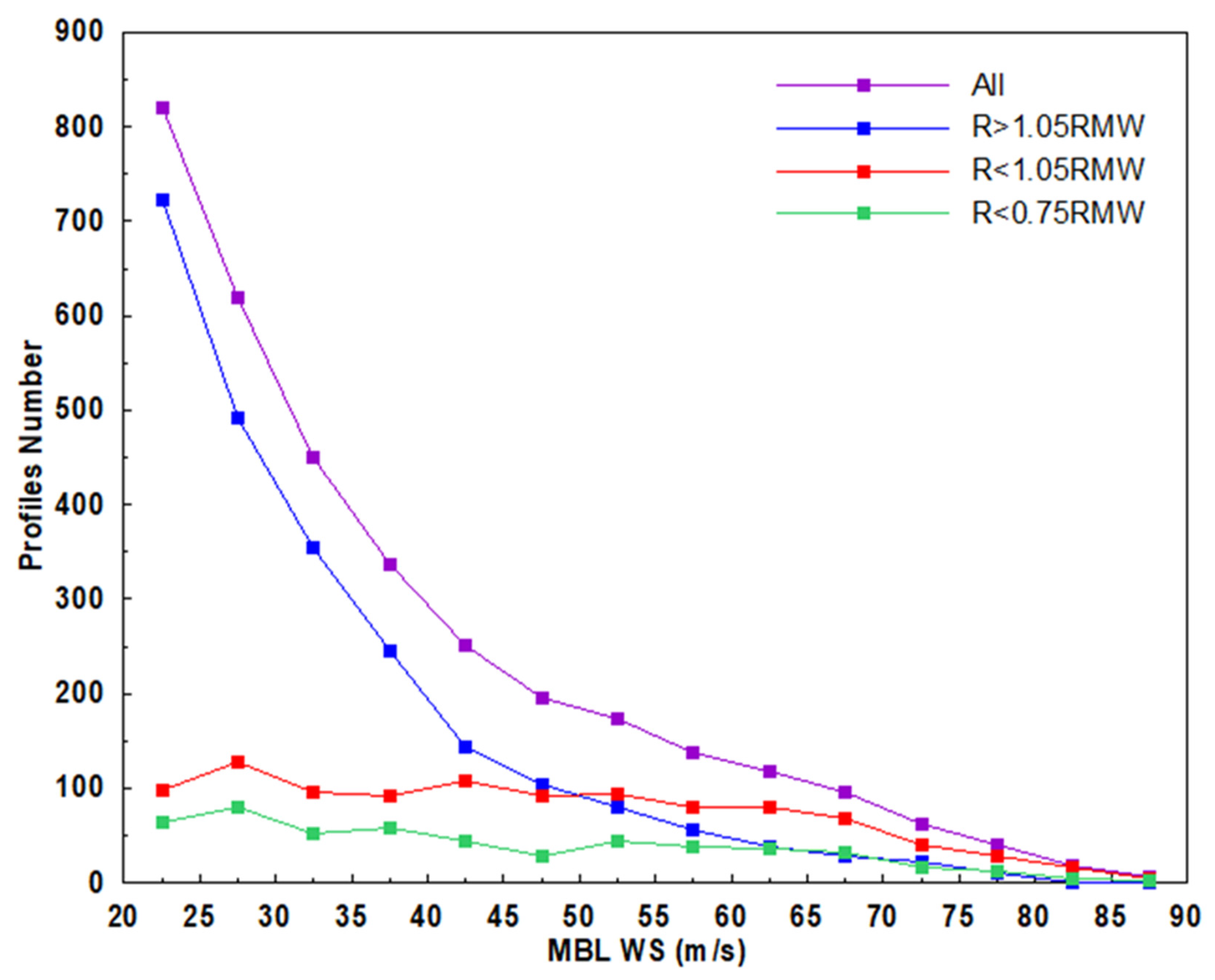
Figure 1. The profile number in each 5 m s−1 MBL mean wind speed bin.
Atmosphere 13 00280 g001
Figure 2. Wind profiles of each MBL mean wind speed group between 20 and 90 m s−1: (a) 20–25 m s−1, (b) 25–30 m s−1, (c) 30–35 m s−1, (d) 35–40 m s−1, (e) 40–45 m s−1, (f) 45–50 m s−1, (g) 50–60 m s−1, (h) 60–70 m s−1, and (i) 70–90 m s−1. The black squares and horizontal bars represent the mean and standard deviation for each height bin. Red lines represent the least square fitting within 20–160 m height. R is the regression coefficient. NUM is the number of dropsonde profiles.
Atmosphere 13 00280 g002
Figure 3. Variation of the friction velocity ( u * , unit: m s−1) with 10-m wind speed ( U 10 , unit: m s−1). The squares with 4 different colors represent the mean value in each wind speed bin from the 4 different R/RMW groups, and vertical bars represent the 95% confidence interval. Black symbols with different shapes represent the results from previous studies including Powell et al. [11], Holthuijsen et al. [16], Richter et al. [27], and Richter et al. [28].
Atmosphere 13 00280 g003
Figure 4. Friction velocity ( u * , unit: m s−1) at every wind speed bin from different R/RMW groups (including all data, and data with R > 1.05RMW, R < 1.05RMW, R < 1.00RMW, R < 0.95RMW, R < 0.90RMW, R < 0.85RMW, R < 0.80RMW, and R < 0.75RMW): (a) 20–25 m s−1, (b) 25–30 m s−1, (c) 30–35 m s−1, (d) 35–40 m s−1, (e) 40–45 m s−1, (f) 45–50 m s−1, (g) 50–60 m s−1, (h) 60–70 m s−1, and (i) 70–90 m s−1. The squares represent the mean value in each wind speed bin, vertical bars represent the 95% confidence interval, and the number above each square is the mean 10 m wind speed of the data. Dashed lines represent the mean value of all data group at each wind speed bin.
Atmosphere 13 00280 g004
Figure 5. Wind profiles of R < 0.85RMW (in red) and R < 0.75RMW (in blue) in different MBL mean wind speed groups, (a) 20–25 m s−1, (b) 25–30 m s−1, (c) 30–35 m s−1, (d) 35–40 m s−1, (e) 40–45 m s−1, (f) 45–50 m s−1, (g) 50–60 m s−1, (h) 60–70 m s−1, and (i) 70–90 m s−1. The squares and horizontal bars represent the mean and standard deviation for each height bin. Lines from top to bottom represent the least square fitting within 20–160 m height. R is the regression coefficient. N is the number of dropsonde profiles.
Atmosphere 13 00280 g005
Figure 6. Same as Figure 3, but for the variation of the surface drag coefficient ( C d × 103) with 10-m wind speed ( U 10 , unit: m s−1). (a) All, R/RMW > 1.05 and R/RMW < 1.05, (b) R/RMW < 0.95, R/RMW < 0.85 and R/RMW < 0.75. The various black symbols are the result from Powell et al. [11], Vickery et al. [30], Holthuijsen et al. [16], Richter et al. [27], and Richter et al. [28].
Atmosphere 13 00280 g006
Table 1. The profile number in each MBL mean wind speed group for different R/RMW ranges.
MBL WS Group
(Unit: m s−1)
R/RMW Range
All>1.05<1.05<1.00<0.95<0.90<0.85<0.80<0.75
20–2582072298928577737064
25–306194911281171131071008880
30–3545035595928783736453
35–4033624591867976716759
40–45251143108928275685744
45–5019610492847465523929
50–603101351751601441281139683
60–70213671461391271171078770
70–901273592797061514135
Sum332222971025941861789708609517
Publisher’s Note: MDPI stays neutral with regard to jurisdictional claims in published maps and institutional affiliations.