Abstract
The Global Navigation Satellite System (GNSS) allows for the cost-effective estimation of the ionospheric total electron content (TEC). However, research on error characteristics of the derived TEC is scarce, which provides insights into the quality of the GNSS ionospheric observation. We investigate characteristics of errors in the derived TEC with data from ~260 GNSS dual-frequency receivers of the Crustal Movement Observation Network of China (CMONOC). The slant TEC is calculated from carrier phase measurements and the vertical TEC over China is fitted with a spatial resolution of 1° by 1° in latitude and longitude in four seasons of 2014. It is found that the errors of both the slant TEC and the derived TEC follow Laplace distribution rather than Gaussian distribution in all seasons. The errors of the slant TEC have sharper peaks than those of the derived TEC. The Mean Absolute Error (MAE) and Root Mean Square Error (RMSE) of the slant TEC are typically 0.04 TECU and 0.2 TECU, while the MAE and RMSE of the fitting residuals for the derived TEC are typically 1 TECU and under 2 TECU, respectively. Both MAEs and RMSEs of the derived TEC have the largest value in spring and the smallest value in summer, while the seasonal dependence is only observed in RMSE of the slant TEC.
1. Introduction
In the last three decades, beacon signals transmitted from global navigation satellite systems (GNSS) have widely been utilized for ionosphere studies. The primary parameter obtained from the satellite beacon signals is the total electron content (TEC), derived from measurements of differential propagation delay and carrier phase between two frequencies, f1 and f2, transmitted from GNSS satellites and propagating through the dispersive ionosphere. A basic problem in TEC derivation is the signal delays in the electronics of satellites and receivers being different for the two frequencies. It is a type of systematic error, which is often referred to as inter-frequency instrumental bias. To remove the instrumental biases, a mathematical model should be established to describe the relations among TEC, biases, and measurements, in which data characteristics and computer resources should also be considered, and then data fitting should be carried out. This makes the TEC derivation a challenging task and efforts never cease to pursue goals, such as better accuracy and faster processing time. Various algorithms have been developed for a single GNSS receiver, small-scale GNSS networks, regional, and global GPS networks. The ionosphere is generally modeled as a thin shell with a spatially smooth distribution of condensed electrons. With functional expressions of TECs in time, latitude, and longitude, equations are built to relate TEC, instrumental biases, and measurements. Then, the equations are solved with numerical computation [1,2,3,4,5,6,7,8,9].
As to the random errors in the derived GNSS TEC, the term “fitting error” is often used to specify the statistical characteristics, since the TEC derivation is essentially the result of data fitting. Most of the available algorithms are based on pseudo-range measurement, which is smoothed with carrier phase for better precision. The fitting error has been reported within ~5 TECU [10,11,12,13]. Recently, ionospheric TEC with an uncertainty lower than 1.0 TECU was achieved by using the carrier phase measurements from the EUREF Permanent Network (EPN) and European Position Determination System (EUPOS) [14]. A root mean square error of 0.40 TECU in TEC derivation was obtained with carrier phase from the dense GNSS Earth Observation Network (GEONET) of Japan [15].
The current fitting errors for GNSS TEC are quantified simply by methods which implicitly assume the random errors follow a normal or Gaussian distribution. However, the error characteristics of GNSS TEC have rarely been addressed or even not verified to be the Gaussian distribution. In construction of the global empirical background TEC model from GNSS TEC Mukhtarov et al. [16] noticed that the probability function of the fitting residuals resembles more of the Laplace distribution than Gaussian distribution. Alternatively, the process of GNSS TEC derivation involves using data from different satellites and receivers. As a matter of fact, it is widely recognized that different equipment can produce widely divergent measurements. Hsu [17] demonstrates that the probability distribution of a mixture of non-uniform Gaussians in air and sea navigation tend to be Laplace with a more pronounced peak and two longer tails. Deviation from Gaussian tends to occur in situations when heterogeneity exists in a large number of observations collected under comparable conditions [18]. Therefore, the ideal assumption of the uniform Gaussian distribution used in GNSS TEC derivation is questionable and needs to be evaluated.
We investigate characteristics of errors in both GNSS measurement and the derived TEC with data from the Crustal Movement Observation Network of China (CMONOC). Section 2 describes the GNSS observations of CMONOC, the grid-based algorithm for deriving TEC from the differential carrier phases between two frequencies of satellite signals, and the error analysis method. Section 3 presents the result from the application of the methods to CMONOC data in 2014. We show the derived TEC with its spatiotemporal variations. Error analysis is made in detail by investigating not only the error distributions, but also the statistical parameters. Summary of the work is given in the last section.
2. Data and Methods
2.1. GNSS Observation
The CMONOC includes ~260 continuous operating GNSS receivers. As shown in Figure 1, it covers a latitude range of 10–53° N, and a longitude range of 75–135° N, respectively. Grids with a size of 1° by 1° in latitude and longitude are divided over CMONOC area. Observations in four seasons around the solstice and equinox are surveyed to check the adaptability of the algorithm. The following dates of 21–23 March, 21–23 June, 21–23 September, and 18–20 December are selected from the year of 2014, on which the geomagnetic activity is low with .
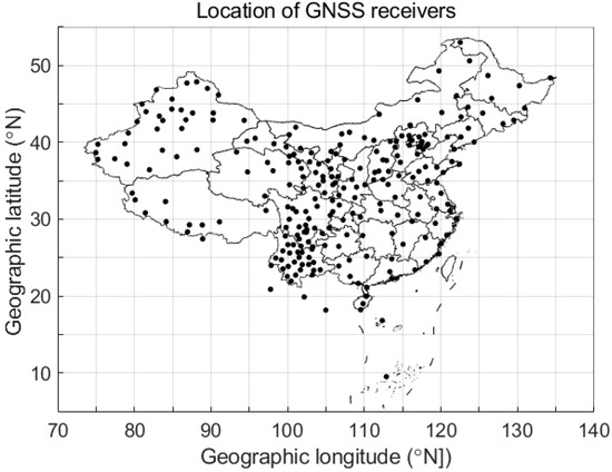
Figure 1.
Geographic location of GNSS receivers of CMONOC.
2.2. Algorithm
As a dispersive medium, the ionosphere causes different group delays and phase advances for radio waves in different frequencies. The group delay and the phase advance are proportional to the TEC along the line of sight. A GNSS receiver measures the pseudo-ranges from satellites to the receiver and the carrier phases of the satellite signals, which provide a mean to obtain TEC.
2.2.1. STEC Measurement and Arc Bias
Having higher precision than that of the pseudo-range, the carrier phase observables L1 and L2 are used to obtain the slant TEC (stec) from a satellite to a receiver.
where k, related to the ionosphere refraction, is 80.62 (m3/s2); λ1 and λ2 are the wavelengths of the two signals; and stec is a relative value, since the instrumental biases and 2π ambiguity are included in the carrier phase measurements. Generally, the instrumental bias can be assumed to be constant for a period of time; the ambiguity does not change in a consecutive measurement (referred to as an arc). Here we define an arc bias, barc, to represent the inter-frequency hardware bias mixed with integer ambiguity. Then the absolute slant TEC, sTEC, can be obtained by taking out the arc bias from the relative stec measurement.
When calculating stec, a data screening step is needed, especially to check cycle-slips in either L1 or L2 phase measurements [19]. If cycle-slips are identified for a certain arc, it would be separated to different arcs, since the 2π ambiguity changes with cycle slip. The arc biases are hence different even though the measurements are taken by the same pair of satellite and receiver.
2.2.2. The Ionosphere Model
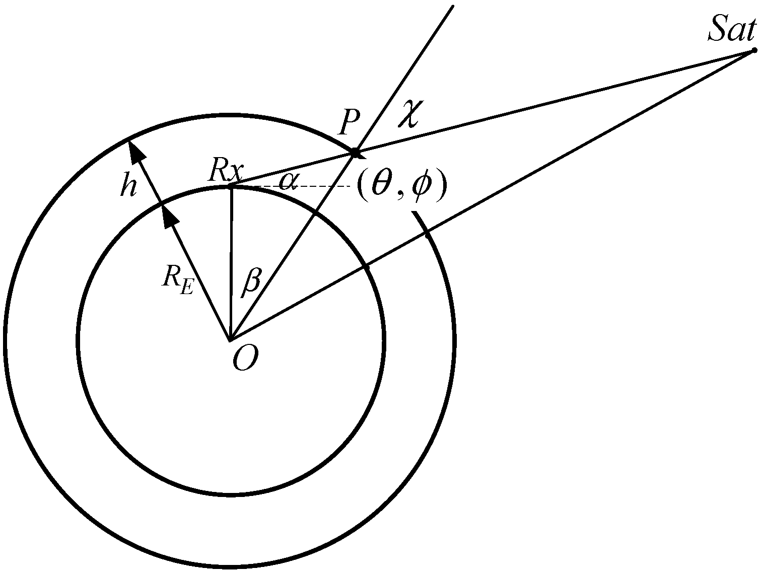
The ionosphere is modeled as a thin shell of a hollow sphere at height h (400 km) and co-centered with the Earth at O, as shown in Figure 2. The line of sight for a satellite and receiver pair crosses the ionosphere at point P, which is called an ionospheric piercing point (IPP). The latitude (φ), longitude (θ), and zenith (χ) of the IPP are related with the satellite and receiver positions as the following,
where, φRx and θRx are the latitude and longitude of the receiver, α and γ are the elevation and azimuth of the satellite, and Re is the Earth radius.
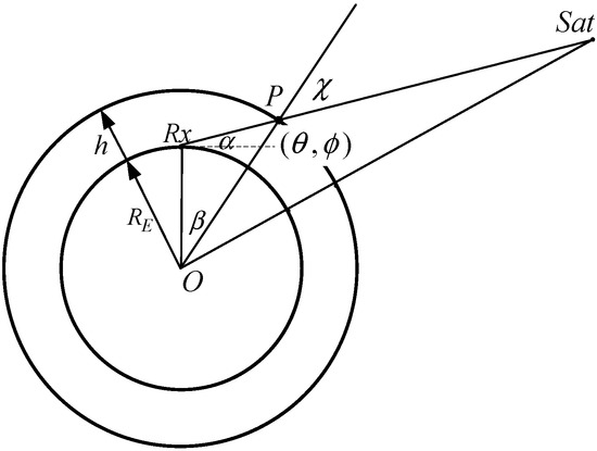
Figure 2.
A schematic of the geometry of a GNSS satellite (Sat), a receiver (Rx), and the ionosphere.
With a smoothly varying assumption of the ionosphere, from the slant TEC given by (2) the vertical TEC at the IPP can be converted as
To suppress the effect of multipath, the cutoff angle for the satellite elevation is set to be 30° when extracting the slant TEC stec and calculating the zenith angle χ.
2.2.3. Matrix Equations Construction
For regional GNSS networks, their receivers tend to be densely distributed in certain areas. The IPPs are accordingly accumulated. With a smoothly varying behavior, the ionospheric TECs at adjacent IPPs would have approximately the same value, which enables functional relations built among slant TECs and arc biases. We divide the ionosphere into grids of the same size over the areas concerned. Further, we assume that the vertical TEC is identical at any point within one grid block at a given time, and the vertical TECs can differ in different grid blocks at the time. Next, mathematical relations among the vertical TEC, arc biases, and the slant TEC can be constructed, as long as two or more than two lines of sight pass through the same grid.
For the signals from satellite j(m) to receiver k(n) we use subscript jk(mn) to denote their consecutive measurement or arc. If their lines of sight propagate through the same grid l at time t of epoch i, the vertical TECs, VTECijk from satellite (j) to receiver (k), and VTECimn from satellite (m) to receiver (n) would be identical. Then using (7), we have the following equations
where, () is the slant TEC from satellite j(m) to receiver k(n) at time t of epoch i, () is the arc bias for the consecutive measurement of satellite j(m) and receiver k(n). A set of equations can be obtained by using a data set from GNSS network, which is expressed in the form of matrix equation as the following:
The coefficient matrix H has only two non-zero elements in every row. The non-zero elements on a column of H come from the same arc. It can be speculated that the columns of H are linearly independent.
2.2.4. Solution of the Matrix Equations
For GNSS observation with 1/30 Hz sampling rate, there are ~20,000 arcs for a network with ~260 receivers in one day. The arcs are increased if cycle slips are detected. Consequently, the number of unknowns is about 20,000, and the number of equations can be over one million with 30° cutoff angle of satellite elevation. Equation (9) is an overdetermined system. It has no solution in the ordinary sense, but rather has a least-squares solution. There are several ways to solve the least-squares problem. The normal equation is the most popular equation, which is obtained by pre-multiplying (9) with the transpose of the coefficient matrix, HT. However, the multiplication amplifies the error in the data, and the computations also accumulate round-off errors. A theoretically equivalent is the singular value decomposition (SVD) approach. The SVD factorizes the coefficient matrix H into two unitary matrices and a diagonal matrix composed of singular values. It is widely used for rank deficient and ill-conditioned matrices [20]. Another solution is determined by the QR factorization of the matrix H. It is more reliable than that of the normal equation if the columns of H are linearly independent [21].
The SVD fixes the round-off problem and produces a best approximation solution in the least squares sense [20]. However, the SVD is computationally expensive. Additionally, memory problems generally occur when creating and handling large matrices directly in MATLAB on desktop computers. Note that the coefficient matrix H in (9) has only two non-zero elements in every row; it can be stored in sparse form and then handled. MATLAB has efficient solving tools based on QR decomposition, which is applicable to a large sparse matrix.
With a QR factorization of H, we have:
Then from (9) and (10) we have the arc biases as given by:
which is the least squares solution of (9). It can be obtained by using matrix left division function of MATLAB.
2.2.5. Program Flowchart
The algorithm is carried out in MATLAB. The corresponding program is named Grid_TEC and developed in MATLAB 2016a (operational in higher versions). The flowchart of Grid_TEC is shown in Figure 3. The inputs are GNSS observations recorded in RINEX format and precise ephemeris of satellites in sp3 format. Carrier phase measurements are read out and stored for each receiver. Possible cycle slip is identified to separate the arc, since it leads 2π ambiguities change in the phase measurements. Next, slant TEC is extracted and stored for each arc. Satellites positions are read out from the sp3 files and interpolated for observation times when the precise ephemeris is not provided. The IPP position is determined by the receiver location and satellite position. The grid size is determined by the network coverage and the density of the receiver. A set of grids is created according to the coverage of IPPs.
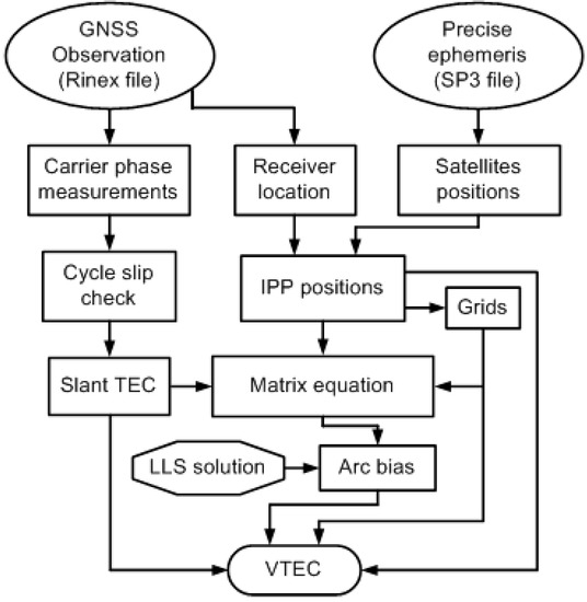
Figure 3.
Flowchart of Grid_TEC algorithm. VTEC over regional GNSS network is derived with the GNSS observation and satellites’ ephemeris.
The matrix equation is built with slant TECs, their IPP positions, and grids information. Next, Linear Least Squares solution of ambiguity combined biases is obtained. VTECs are calculated from slant TEC and stored with grids according to their IPP positions.
2.3. Error Analysis Method
We analyze two kinds of measurement dealt with in the Grid_TEC algorithm. The first concerns the input, which is stec from (1). The second is the output VTEC in (7), which is related with the input stec and the fitting result of arc bias.
2.3.1. Error Estimation
An error is the difference between the observed or calculated value of a quantity and its true value. Since a true value for any measurable quantity is not known, an average of many repeated independent measurements is used to replace true value. However, it is impossible to repeat measurements in many practical observations where the measured quantity varies with time. A moving average or running mean is often used.
The measurement error of stec is estimated by examining the dispersion of the stec to its running mean,
For the GNSS observation with a 30-s resolution, Δsteci is calculated by taking the standard deviation of stec for 5-min interval (11 consecutive epochs).
Concerning the error of the derived VTEC, we can take the residual defined by the difference between the left-hand-side and the right-hand-side of (8), which assumes the identity of two VTECs within a grid.
The smaller is the better the assumption and the fitting are.
2.3.2. Statistical Characteristics
The statistical parameters, the median of the error (), mean absolute error (MAE, ), and root mean square error (RMSE, ), are used to qualify the observation and fitting result. With representing the general error, the statistical parameters are calculated by
where, N is the amount of the observations or number of the equations in (9). The MAE result will always be smaller or equal to the RMSE. Their difference demonstrates the variance in the individual errors. The ratio of the MAE to the RMSE is a fixed value for a certain dataset. Both RMSE and MAE are important to error analysis [22]. It should be noted that the MAE is mostly suitable to describe uniformly distributed errors. When using the RMSE a normal (Gaussian) distribution is generally an underlying assumption.
Generally, the errors are assumed to follow Gaussian distributions, since it is the most important probability distribution in statistics, which fits many natural phenomena. The MAE is related with the RMSE by () for Gaussian distribution. However, practical data and its processing result would not follow an ideal Gaussian distribution. We also use histograms to graphically show the distributions of the errors. Proper distributional model can be estimated with probability plot.
3. Results
Following the flowchart of Grid_TEC algorithm, data processing is made on a daily base. The number of established equations is about 1.5 million and the number of unknowns is about 15 thousand. It takes about 25 min to run the program, from reading the GNSS data to solving the Equation (11), by a desktop computer (PC) using an Intel® Core I i7-700 CPU.
3.1. Derived VTEC
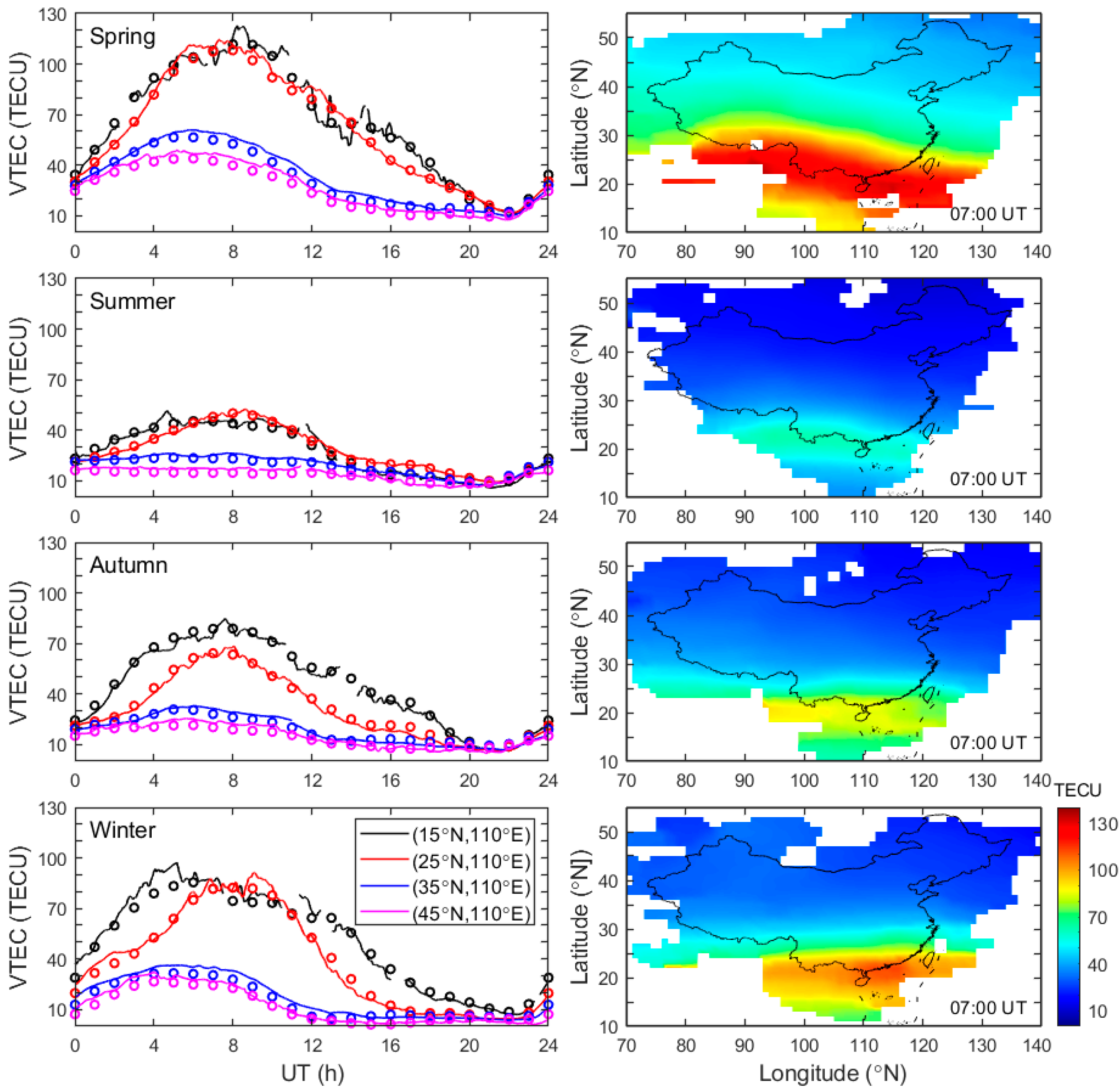
With the bias given by (11), VTEC is calculated from (7). Figure 4 presents the derived VTEC in two forms. The left column is diurnal variation of VTEC in four seasons of 2014 at the meridian 110° E. VTECs at four latitudes, 15° N (black), 25° N (red), 35° N (blue), and 45° N (magenta) are given to observe the latitudinal variation. The circles are VTECs derived with spherical harmonics analysis by using data from a chain of receivers at the meridian 110° E [23]. The right column is TEC maps in China at 07:00 universal time (UT) of the four seasons of 2014.
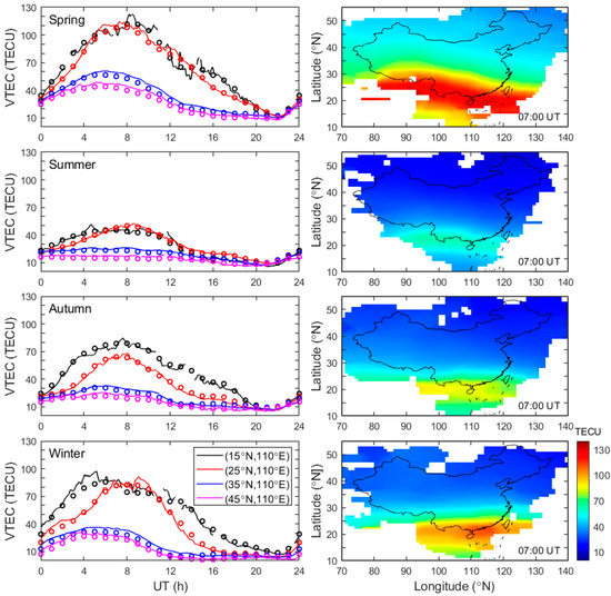
Figure 4.
VTEC temporal variation at 110° E and TEC map at 7:00 UT.
Concerning the diurnal variation, the variations of VTEC both in line and circle shows a high degree of conformity. Note that the local time (LT) at 110° E is ~7.3 h advanced. VTEC reaches its peak at ~12:30–15:30 LT in China sector. The peak appears at an earlier time with the increase of latitude. The value of the peak at low latitude is much larger than that at middle latitude, implying a large gradient from 25° N to 35° N. VTEC gets to a valley at ~21:00–22:00 LT, with insignificant latitudinal difference. Seasonal variation is remarkable. VTEC is larger in equinoxes than in summer. The peak value of VTEC in spring can be close to 130 TECU, while it is around 60 TECU in summer. It is noteworthy that VTECs in daytime are larger in winter than in autumn. This agrees with previous studies, which attribute the result to greater contribution from plasmasphere.
The TEC map shows more details of the spatial variation of VTEC. The longitudinal range from 70 to 140° E at 7:00 UT corresponds to 11:40~16:20 LT. Latitudinal variation or VTEC latitude gradient is conspicuous, due to the equatorial ionization anomaly (EIA), which centered around 20° N. The magnitude and latitudinal range of the EIA are the largest in spring. They are the smallest in summer, and larger in winter than autumn. If converting the longitude into LT, the largest latitude EIA reaches ~25° N at the time between 12:30 and 13:00 LT in spring. The location of EIA crest does not change significantly in other seasons.
3.2. Error Analysis
Error analysis is carried out by using the definitions and procedures described in the above error analysis method.
3.2.1. Measurement Error
The measurement error Δsteci is estimated with (12) over a 5-min running window for all receivers. Table 1 gives the statistical parameters based on three days for each season in 2014. The biases of the errors are 0 for all the seasons. The MAE is 0.04 TECU, except for autumn when the MAE is 0.03 TECU. The RMSE is typically ~0.2 TECU, from 0.12 TECU in summer to 0.22 TECU in spring. It is 0.19 TECU in winter, larger than that of 0.15 TECU in autumn. Therefore, the RMSE is different among different seasons though the MAE is the same as or equal to one another. Moreover, it is noteworthy that is much smaller than . The typical ratio of is 0.2. This indicates that the measurement errors do not follow the normal distribution.

Table 1.
Statistical parameters of measurement errors in 2014.
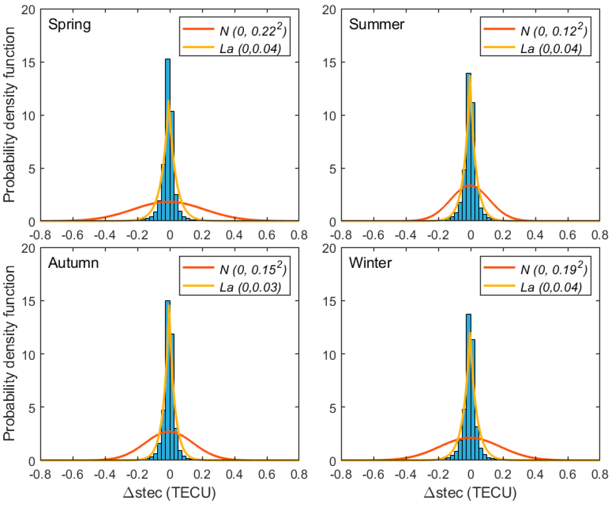
To examine the error characteristics, Figure 5 presents the normalized frequency distribution of stec measurement errors with a bin of 0.025 TECU for the four seasons of 2014. Nearly symmetrically, each histogram peaks sharply around the center, then decreases steeply to a low level and spreads noticeably afterwards to both sides. The error distribution is found to follow a double exponential or Laplace distribution rather than a Gaussian distribution. The probability density function of Gaussian distribution is associated with the median and RMSE parameters.
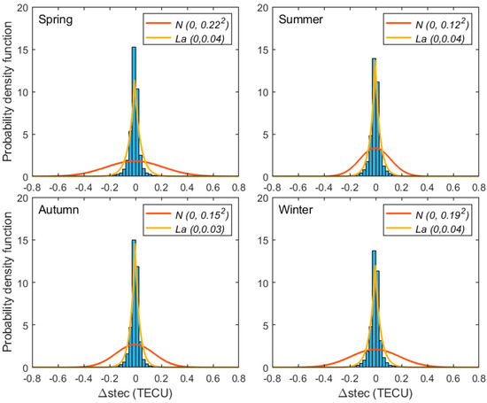
Figure 5.
Error distribution of stec measurements in 2014. Overlaid are Gaussian (red) and Laplace (orange) probability density function.
The Laplace distribution can be expressed with the median and MAE.
We use and to express the Gaussian and Laplace distributions with statistical parameters, respectively. As shown in Figure 5, the stec error distributions in the four seasons are fitted by curves of Laplace distribution (in orange) quite closely. They differ from Gaussian distribution (in red) greatly.
Table 2 lists the cumulative probability (%) of the measurement errors for the typical ranges in four seasons of 2014. Theoretically, the cumulative probability for Laplace distribution is 63.2%, 86.5%, and 95.0% for , , and ranges. It can be seen that the cumulative probability of Δstec is larger than that of theory within and . It agrees with that of the theory for . For an ideal Laplace distribution, we have . The in Table 1 ranges from 0.19 to 0.33, which are smaller than 0.5. The measurement error has a sharper peak and shorter tails than the ideal Laplace distribution.

Table 2.
Cumulative probability (%) of Δstec in four seasons of 2014.
It is widely recognized that different equipment can produce widely divergent measurements. Hsu [17] demonstrates that the probability distribution of a mixture of non-uniform Gaussians in air and sea navigation tend to be Laplace with a more pronounced peak and two longer tails. Deviation from Gaussian tends to occur in situations when heterogeneity exists in the population [18]. This can explain the Laplace distribution of the errors in slant TEC measurement, since the noise level of different satellite-receiver pair is affected by both the hardware and space environment, which are different from one another.
3.2.2. Error of the Derived TEC
The error of VTEC is calculated with (13). Table 3 lists the statistical parameters of the residuals in the four seasons of 2014. The bias of the fitting errors, , is 0 for all seasons. The MAE, , is in 1 TECU level. In spring/summer it is 1.12/0.70 TECU, which is the largest/smallest in the four seasons. is 0.87/0.89 TECU in autumn/winter. The RMSE, , has the same dependence on seasons as . It is under 2 TECU for all seasons. It is 1.94/1.12 TECU in spring/summer, which is the largest/smallest. is 1.46 TECU and 1.60 TECU in autumn and winter, respectively. For residuals is not equal to either. is about 0.6, which is smaller than that of Gaussian distribution and larger than that of Laplace distribution. Therefore, the fitting errors do not follow the normal distribution even though they are unbiased.

Table 3.
Statistical parameters of ΔVTEC in 2014.
Figure 6 presents the normalized frequency distribution with a bin of 0.5 TECU for the residuals in the four seasons of 2014. Overlaid are curves for probability density functions of Gaussian distribution () in red, and Laplace distribution () in orange, respectively. The fitting residuals resemble Laplace distribution more than Gaussian distributions.
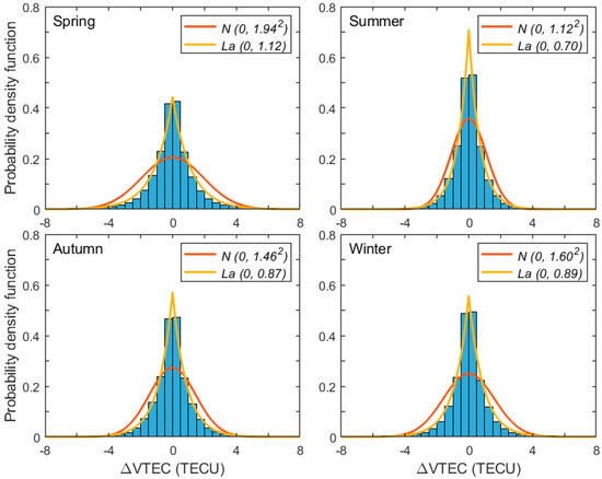
Figure 6.
Histograms of residuals overlaid with Gaussian (red) and Laplace distribution curves (orange).
Table 4 lists the cumulative probability (%) of the fitting errors for the typical ranges in four seasons of 2014. The cumulative probability tends to be the similar level for different seasons. They generally agree with those of ideal Laplace distribution, especially for and ranges. With RMSE, 80.9%, 95.1%, and 97.8% of errors fall within , , and , respectively. Noting that for Gaussian distribution it is 68.3%, 95.5%, and 99.7%, respectively, there are ~13% more errors fall in , there are ~2% more cases outside . The result indicates that most of the derived VTEC have an error less than , however, the outliers of tend to be 2%. It can be seen that both MAE and RMSE are important parameters to characterize the errors deviate from Gaussian distribution. A smaller value of means larger deviation from Gaussian distribution and less outliers outside .

Table 4.
Cumulative probability (%) of ΔVTEC in four seasons of 2014.
The error of the VTEC follows the Laplace distribution as that of stec does since the VTEC is derived from stec. In evaluation of the global TEC maps from GNSS derived TEC, Mukhtarov et al. reported that the probability function of the residuals follows the Laplace distribution rather than Gaussian distribution [16]. However, the peak of the distribution for VTEC is not as sharp as that of stec. Both of the MAE and RMSE for VTEC are much larger than those for stec. It is reasonable to speculate that the assumption used in the TEC derivation should be responsible. Simulation should be needed to clarify how the error characteristics of the derived VTEC vary with the ionospheric model and the measurement error.
4. Summary
We develop the Grid_TEC algorithm for deriving TEC with carrier phase observables from regional GNSS networks. The ionosphere over the area of the network is divided into grids with the same size. A set of equations is established to relate the vertical TEC in each grid with the observations. The equations are solved with QR decomposition. Written in MATLAB, the algorithm can be run in a desktop computer, conveniently. The performance of the Grid_TEC is evaluated by applying it to data of 2014 from CMONOC Network of China and making error analysis of the measurement and the fitting result. The TEC over China is derived with a spatial resolution of 1° by 1° in latitude and longitude. Daily and seasonal variations of TEC are observed. The north crest of the equatorial anomaly is captured with TEC map, which also display seasonal variations.
The error characteristics of both the measured stec and the derived VTEC are investigated. While the MAE and RMSE of the slant TEC error are typically 0.04 TECU and 0.2 TECU, the MAE and RMSE of the fitting residuals for VTEC are typically 1 TECU and under 2 TECU, respectively. Both the error distributions of the GNSS measurement and the derived TEC follow Laplace distribution rather than Gaussian distribution. The error distribution for the slant TEC has a sharper peak and shorter tails than the ideal Laplace distribution. The distribution of the fitting residuals has a sharper peak and longer tails than Gaussian distribution. Both MAE and RMSE are useful to represent the error characteristics. A smaller ratio of MAE to RMSE, , leads to a sharper peak and two shorter tails of the distribution. The ratio of MAE to RMSE can also be used to indicate how much the error distribution deviates from Gaussian. The smaller the value of is, the lager deviation of the distribution from Gaussian. Moreover, there tends to have less outliers outside for a smaller value of .
Author Contributions
Conceptualization: G.M.; methodology: G.M. and J.F.; software: G.M., J.L. and Q.W.; formal analysis: G.M.; writing—original draft preparation: G.M.; writing—review and editing: G.M.; project administration: G.M. All authors have read and agreed to the published version of the manuscript.
Funding
This research was funded by the National Natural Science Foundation of China, grant number 12073049, U2031146 and 11873064.
Institutional Review Board Statement
Not applicable.
Informed Consent Statement
Not applicable.
Data Availability Statement
Not applicable.
Acknowledgments
We thank CMONOC for providing the GNSS data used for this study.
Conflicts of Interest
The authors declare no conflict of interest.
References
- Lanyi, G.E.; Roth, T. A comparison of mapped and measured total ionospheric electron content using Global Positioning System and beacon satellites observations. Radio Sci. 1988, 23, 483–492. [Google Scholar] [CrossRef]
- Mannucci, A.J.; Wilson, B.D.; Yuan, D.J.; Ho, C.H.; Lindqwister, U.J.; Runge, T.F. A global mapping technique for GPSderived ionospheric electron content measurements. Radio Sci. 1998, 33, 565–582. [Google Scholar] [CrossRef]
- Hernández-Pajares, M.; Juan, J.M.; Sanz, J. New approaches in global ionospheric determination using ground GPS data. J. Atmos. Sol.-Terr. Phys. 1999, 61, 1237–1247. [Google Scholar] [CrossRef]
- Otsuka, Y.; Ogawa, T.; Saito, A.; Tsugawa, T.; Fukao, S.; Miyazaki, S. A new technique for mapping of total electron content using GPS network in Japan. Earth Planets Space 2002, 54, 63–70. [Google Scholar] [CrossRef]
- Brunini, C.; Meza, A.; Azpilicueta, F.; Van Zele, M.A.; Gende, M.; Diaz, A. A New Ionosphere Monitoring Technology Based on GPS. Astrophys. Space Sci. 2004, 290, 415–429. [Google Scholar] [CrossRef]
- Arikan, F.; Nayir, H.; Sezen, U.; Arikan, O. Estimation of single station interfrequency receiver bias using GPS-TEC. Radio Sci. 2008, 43, RS4004. [Google Scholar] [CrossRef]
- Zhang, D.H.; Zhang, W.; Li, Q.; Shi, L.Q.; Hao, Y.Q.; Xiao, Z. Accuracy analysis of the GPS instrumental bias estimated from observations in middle and low latitudes. Ann. Geophys. 2010, 28, 1571–1580. [Google Scholar] [CrossRef]
- Choi, B.K.; Park, J.U.; Roh, K.M.; Lee, S.J. Comparison of GPS receiver DCB estimation methods using a GPS network. Earth Planets Space 2013, 65, 707–711. [Google Scholar] [CrossRef][Green Version]
- Prasad, R.S.; Kumar, S.; Jayachandran, P.T. Receiver DCB estimation and GPS vTEC study at a low latitude station in the South Pacific. J. Atmos. Sol. -Terr. Phys. 2016, 149, 120–130. [Google Scholar] [CrossRef]
- Ma, G.; Maruyama, T. Derivation of TEC and estimation of instrumental biases from GEONET in Japan. Ann. Geophys. 2003, 21, 2083–2093. [Google Scholar] [CrossRef]
- Hernández-Pajares, M.; Juan, J.M.; Sanz, J.; Orus, R.; Garcia-Rigo, A.; Feltens, J.; Komjathy, A.; Schaer, S.C.; Krankowski, A. The IGS VTEC maps: A reliable source of ionospheric information since 1998. J. Geod. 2009, 83, 263–275. [Google Scholar] [CrossRef]
- Alizadeh, M.M.; Schuh, H.; Todorova, S.; Schmidt, M. Global ionosphere maps of VTEC from GNSS, satellite altimetry, and Formosat-3/COSMIC data. J. Geod. 2011, 85, 975–987. [Google Scholar] [CrossRef]
- Roma-Dollase, D.; Hernández-Pajares, M.; Krankowski, A.; Kotulak, K.; Ghoddousi-Fard, R.; Yuan, Y.; Li, Z.; Zhang, H.; Shi, C.; Wang, C.; et al. Consistency of seven different gnss global ionospheric mapping techniques during one solar cycle. J. Geod. 2018, 92, 691–706. [Google Scholar] [CrossRef]
- Krypiak-Gregorczyk, A.; Wielgosz, P. Carrier phase bias estimation of geometry-free linear combination of GNSS signals for ionospheric TEC modeling. GPS Solut. 2018, 22, 45. [Google Scholar] [CrossRef]
- Li, Q.; Ma, G.; Maruyama, T.; Li, J.; Wan, Q.; Wang, X.; Fan, J.; Zhang, J. High-precision VTEC derivation with GEONET. Earth Planets Space 2000, 72, 14. [Google Scholar] [CrossRef]
- Mukhtarov, P.; Pancheva, D.; Andonov, B.; Pashova, L. Global TEC maps based on GNNS data: 2. Model evaluation. J. Geophys. Res.-Space phys. 2013, 118, 4609–4617. [Google Scholar] [CrossRef]
- Hsu, D.A. Long-tailed distributions for position errors in navigation. Appl. Stat. 1979, 28, 62–72. [Google Scholar] [CrossRef]
- Geraci, M.; Borja, M.C. Notebook: The Laplace distribution. Significance 2018, 15, 10–11. [Google Scholar] [CrossRef]
- Blewitt, G. An automatic editing algorithm for GPS data. Geophys. Res. Lett. 1990, 17, 199–202. [Google Scholar] [CrossRef]
- Press, W.H.; Teukolsky, S.A.; Vetterling, W.T.; Flannery, B.P. Numerical Recipes in Fortran 77; Cambridge University Press: Cambridge, UK, 1992; pp. 670–673. [Google Scholar]
- Lay, D.C.; Lay, S.R.; McDonald, J.J. Linear Algebra and Its Applications; Pearson: London, UK, 2016. [Google Scholar]
- Chai, T.; Draxler, R.R. Root mean square error (RMSE) or mean absolute error (MAE)?—Arguments against avoiding RMSE in the literature. Geosci. Model. Dev. 2014, 7, 1247–1250. [Google Scholar] [CrossRef]
- Wan, Q.; Ma, G.; Li, J.; Wang, X.; Lu, W.; Maruyama, T.; Fan, J.; Zhang, J. Performance evaluation of IRI-2016 with GPS-derived TEC at the meridian of 110° E in China of 2014. J. Atmos. Sol. -Terr. Phys. 2020, 201, 105206. [Google Scholar] [CrossRef]
Publisher’s Note: MDPI stays neutral with regard to jurisdictional claims in published maps and institutional affiliations. |
© 2022 by the authors. Licensee MDPI, Basel, Switzerland. This article is an open access article distributed under the terms and conditions of the Creative Commons Attribution (CC BY) license (https://creativecommons.org/licenses/by/4.0/).


