Kelvin Wave and Its Impact on the Venus Atmosphere Tested by Observing System Simulation Experiment

Abstract

At the cloud top of the Venus atmosphere, equatorial Kelvin waves have been observed and are considered to play an important role in the super-rotation. We were able to reproduce the wave in a general circulation model (GCM) by conducting an observing system simulation experiment (OSSE) with the help of a data assimilation system. The synthetic horizontal winds of the Kelvin wave produced by the linear wave propagating model are assimilated at the cloud top (~70 km) in realistic conditions, assuming they are obtained from cloud tracking of ultra-violet images (UVI) taken by the Venus orbiters. It is demonstrated using Eliassen–Palm (EP) fluxes that the reproduced Kelvin wave transports angular momentum and plays an important role in the magnitude and structure of the super-rotation, causing the acceleration and deceleration of zonal wind of ~0.1 m/s day⁻¹. The conditions required in order to reproduce the Kelvin wave have also been investigated. It is desirable to have 24 hourly dayside satellite observations in an equatorial orbit, such as the Akatsuki Venus climate orbiter. The results of this type of data assimilation study will be useful in the planning of future observation missions to the atmospheres of planets.

1. Introduction

Venus is covered by a thick cloud at altitudes of around 45–70 km, and therefore, it is difficult to observe the atmosphere below the cloud from space directly. At the cloud top (~70 km), planetary-scale wave patterns are intermittently observed and considered to be Kelvin and Rossby waves, based on their structures and periods [1,2,3,4]. The Kelvin wave in the equatorial region propagates faster than the super-rotation, with a fast zonal flow of ~100 m/s at the cloud top, e.g., [5,6], with a period of ~4 Earth days, while the Rossby wave in mid-latitudes does slower with a period of ~5 Earth days [7,8]. While these waves are considered to play an important role in the maintenance of the super-rotation through their momentum transport, they, particularly the Kelvin wave, are not well reproduced in Venus’s general circulation models (GCMs).

Recently, the first data assimilation system for the Venus atmosphere was developed by the use of the Local Ensemble Transform Kalman Filter (LETKF) [9]. In this system, ensemble forecasts are performed by the Venus GCM named AFES-Venus [10], based on AFES (an atmospheric GCM for the Earth Simulator) [11]. Observing system simulation experiments (OSSEs) to reproduce Kelvin waves were conducted in the previous work [12] using this AFES LETKF Data Assimilation System for Venus named ALEDAS-V [13]. However, because synthetic observations were produced by another Venus GCM [14], whose basic state was greatly different from that of AFES-Venus, significant inconsistency between the models occurred during data assimilation. Then the impact of the Kelvin wave on the general circulation could not be investigated satisfactorily. Furthermore, the longitudinal range of observations was not limited, though actual ultra-violet images (UVI) can be obtained by satellites in a limited region on the dayside.

As an extension of the previous study [12], here, we will reproduce the Kelvin wave more realistically and completely by the OSSE using ALEDAS-V and investigate its impact on the Venus atmosphere. The synthetic observations of horizontal winds are created by the linear wave propagating model [15,16], in which the basic state is adjusted to be similar to that of AFES-Venus. The necessary conditions to reproduce the Kelvin wave are also investigated in a realistic way by the dayside observation from satellites. This paper is organized as follows: Experimental settings of OSSEs are described in Section 2. Section 3 presents the results of the reproduced Kelvin wave and its impact, as well as the conditions required to reproduce the Kelvin wave. Section 4 contains a summary and discussion.

2. Experimental Settings

Synthetic observations for OSSEs are produced by the linear wave propagating model [15,16], with the basic state similar to that of AFES-Venus (see Figure A1). In the model, the Kelvin wave is forced at the bottom of 60 km, assuming upward propagation of the Kelvin wave from a lower altitude. Then the Kelvin wave propagation in the given basic state is calculated by a linearized primitive equation. The horizontal resolution is 120 times 58 in a latitude–longitude grid system with constant 3-degree intervals for each direction, which is comparable to that obtained by the Akatsuki orbiter [17,18]. Horizontal winds obtained at the cloud top (70 km) in this model are used for data assimilation, by which the Kelvin wave with a period of ~4 Earth days is induced in the equatorial region (see Figure A2). These settings are consistent with horizontal winds derived from UVI taken by the Akatsuki orbiter [18]. Here, we have prepared a series of synthetic observations, in which observation conditions are systematically changed. We chose 6-Earth-hourly dayside observations in low-latitudes as a control case, covering 120° (zonal width of 8 h in local time; LT) in longitude from 120° E (east) (8 LT) to 120° W (west) (16 LT) and 60° in latitude from 30° S (south) to 30° N (north). Akatsuki may observe similar regions with a comparable frequency throughout good seasons of observation [17]. It is worth noting that the direction of planetary rotation is the same as that of the Earth in this study.

ALEDAS-V uses LETKF [9] and AFES-Venus [10] for data assimilation and ensemble forecast, respectively. The number of ensemble members is 31. In LETKF, ensemble forecasts are updated by assimilating horizontal wind observations. The assimilation cycle is 6-Earth-hourly, and observations are assigned to each Earth-hour if they are available. The parameters explained below were chosen from previous research [12,13,19,20]. The observed error is assumed to be 3 m/s, and the horizontal and vertical localization parameters are 400 km and $\log P=0.4$, respectively, where P is the pressure of the given observations. The multiplicative 10% spread inflation is used for background error covariance [9]. AFES-Venus solves a dry full nonlinear primitive equation in a spherical domain. The horizontal resolution is 128 times 64 in the latitude–longitude grid system, and the vertical layers are 60 with almost constant ~2 km intervals up to 120 km. Physical parameters such as radius, rotation period, gravity acceleration, specific heat, and so on are set to values for Venus. While the value of specific heat varies 740–1180 J Kg⁻¹ K⁻¹ [21], it is fixed at a constant value of 1000 J Kg⁻¹ K⁻¹ for simplicity. Solar heating and infrared cooling are simplified by a solar net flux profile based on [22] and Newtonian cooling [23], respectively. It should be noted that while some Venus GCMs implemented a radiative transfer scheme [24,25], we will use this experimental setting for simplicity. Topography and planetary boundary layer are not considered. At the planetary surface, Rayleigh friction with a damping time of ~0.5 Earth days is used. Above 80 km in the high atmosphere, there is a sponge layer that solely acts on eddy components. The T42 (triangular truncation at wavenumber 42) dynamical core additionally implements vertical eddy diffusion with 0.15 m²/s and horizontal eddy diffusion with a 4th-order elliptic operator (squared Laplacian) viscosity with a damping time of ~0.1 Earth day at the maximum wavenumber. In order to focus on the Kelvin wave, the diurnal component of solar heating and hence thermal tides are excluded [26] in both idealized observations and AFES-Venus.

From an idealized initial condition of the super-rotation, AFES-Venus spins up for 4 Earth years. The initial condition is a temperature field with low static stability layers that is gradient wind balanced with the idealized initial super-rotation. It should be noted that the general circulation obtained in AFES-Venus in a quasi-equilibrium state is consistent with previous observations, e.g., [27,28] in many aspects: The zonally averaged zonal wind has a weak mid-latitude jet and almost constant velocity of about 120 m/s in latitudes between 45˚ S and 45˚ N at the cloud top-level [29], structures of cold collar [30], thermal tide [31,32], planetary-scale streak [33], and small-scale gravity waves [34]. From 1 January, 5th year, data assimilation is performed for one Earth month. We will compare OSSE (control case) results with the AFES-Venus free run forecast (frf case) in which no observations are assimilated. Previous studies [10,13,19,31] go into greater detail about the AFES-Venus and ALEDAS-V experimental setups.

3. Results

In this section, we shall compare the results of OSSE (control case) to those of the free-run forecast (frf case). Section 3.1 presents the time evolution of the Kelvin wave. By composite means in Section 3.2, we extract structures from the Kelvin wave. The impact of the Kelvin wave on the general circulation is investigated in Section 3.3. Finally, the necessary conditions to reproduce the Kelvin wave by actual satellite observations are discussed in Section 3.4.

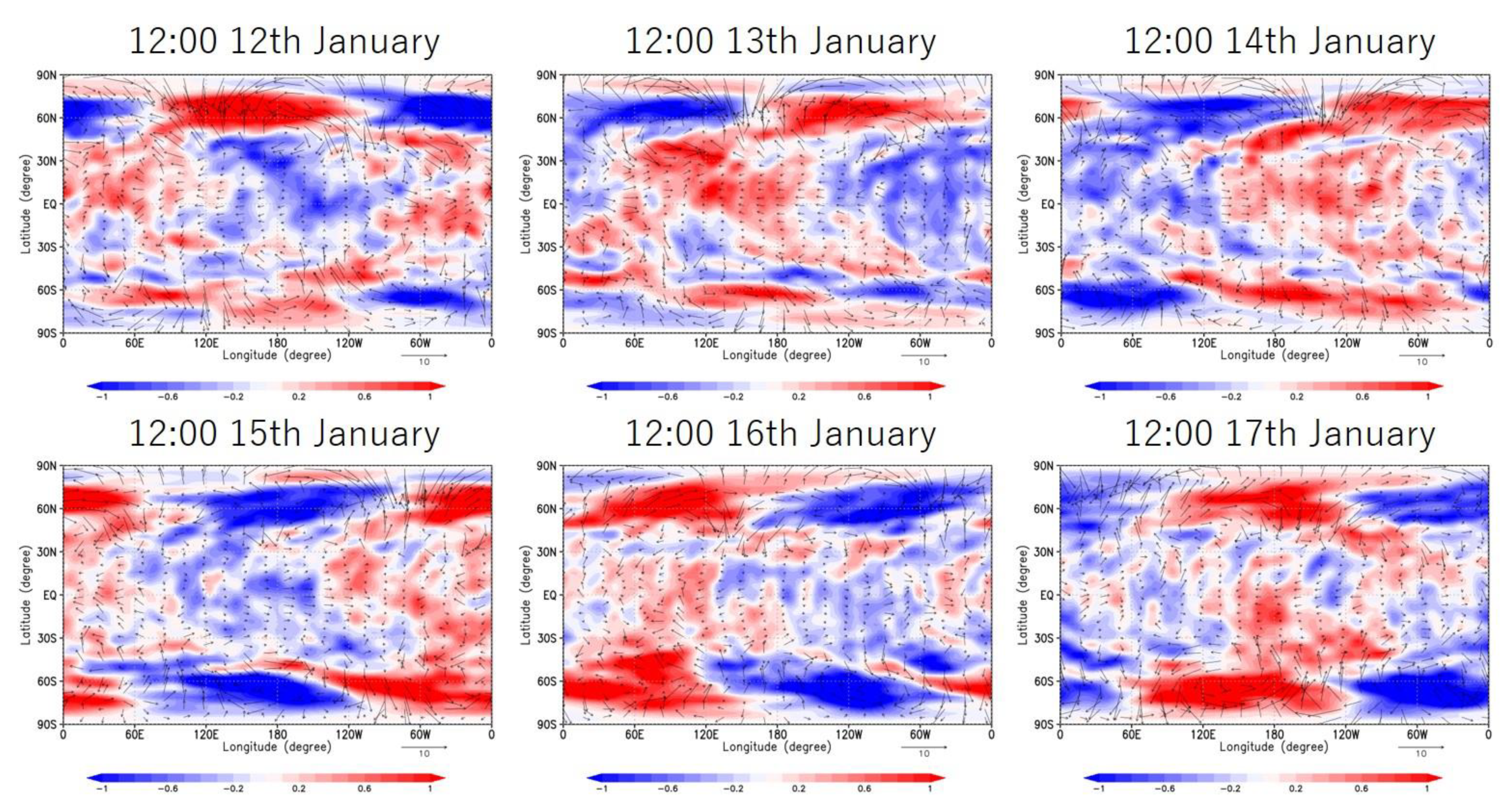
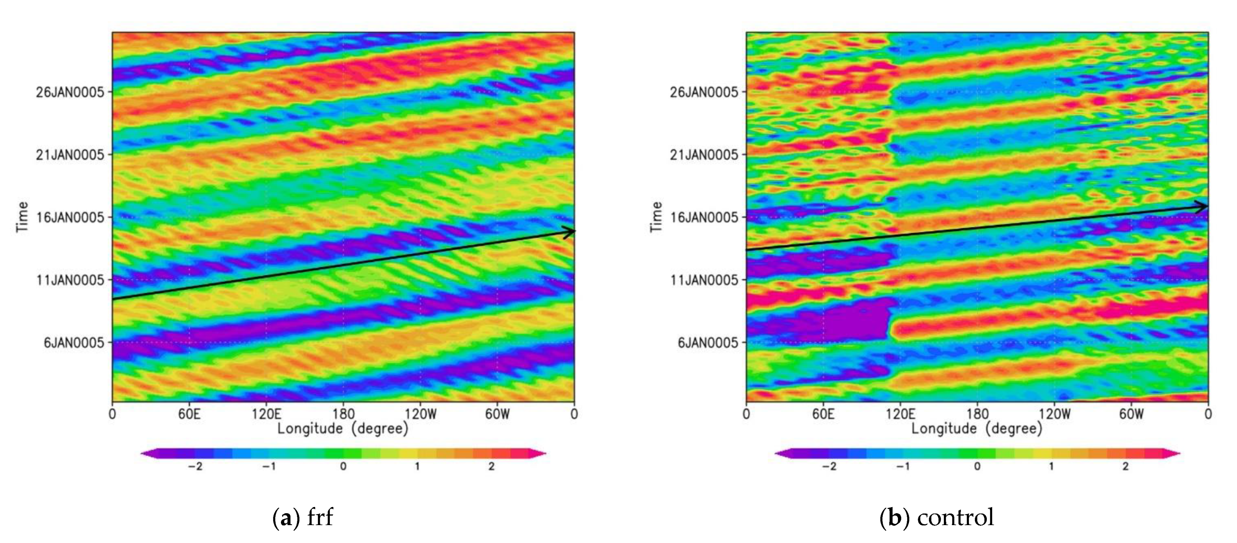
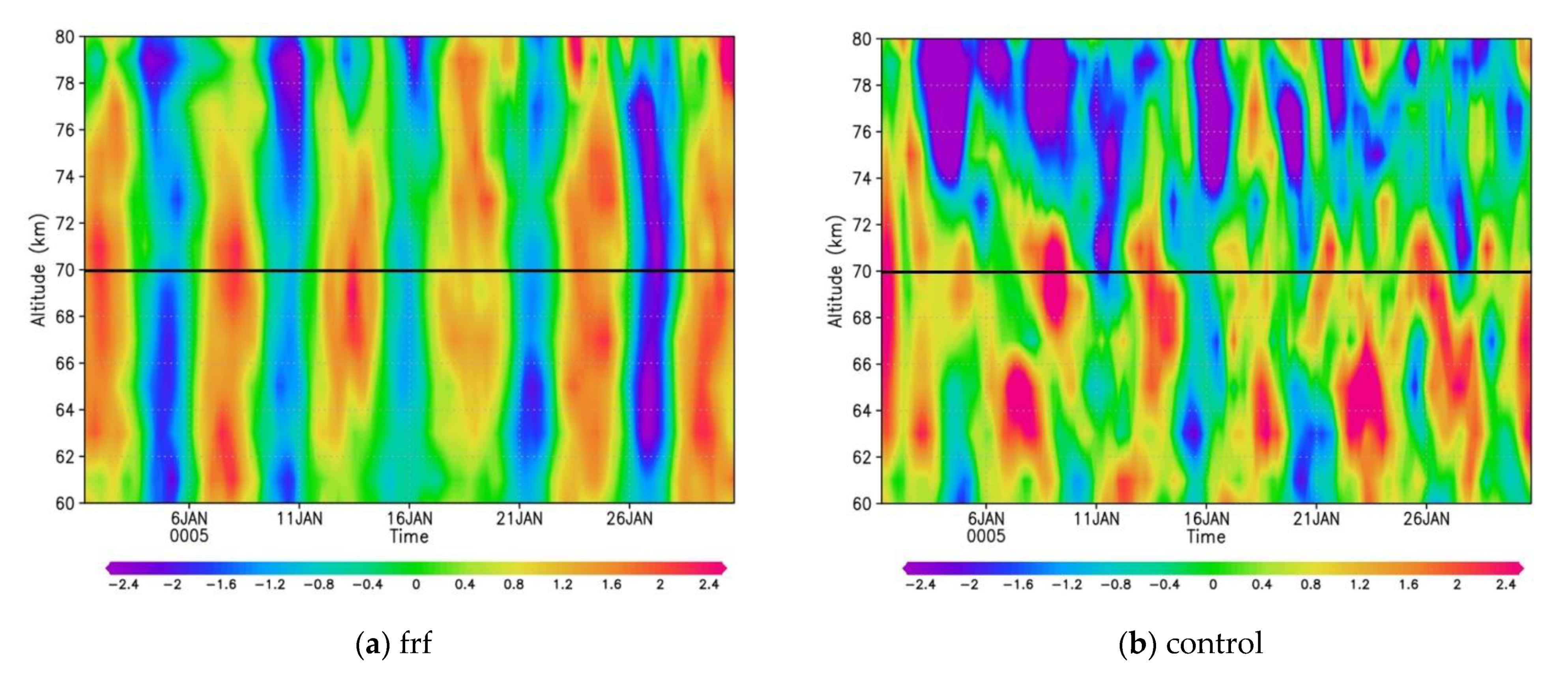
3.1. Time Evolutions

First, time evolutions of horizontal structure at the cloud top (~70 km) for the control case are shown in Figure 1. The Kelvin wave, with a period of ~4 Earth days, is reproduced in the equatorial region in both the zonal wind and temperature components successfully by the horizontal wind assimilation. See also: Animations for the control and frf examples may be seen in Videos S1 and S2, respectively. The Kelvin wave’s phase in the zonal wind is zonally shifted from that in temperature, indicating that the Kelvin wave propagates vertically [35]. Because the LETKF algorithm uses a covariance matrix that includes horizontal winds and temperature, the temperature is also updated to show that its uncertainty is limited.

In order to confirm when the Kelvin wave is clearly reproduced during the time evolution of OSSE, longitude-time cross-sections of the zonal wind deviation from its time average at the equator and 70 km altitude are shown in Figure 2 for the (a) frf and (b) control cases. Black arrows indicate periods of ~5 and ~4 Earth days for the frf and control cases, respectively. The Kelvin wave, with a period of ~4 Earth days, is clearly reproduced only for the control case. The Kelvin wave seems to appear where horizontal winds are assimilated within 120° E–120° W in longitudes immediately after OSSE starts. However, it does not propagate sufficiently in the longitudinal direction, resulting in a discontinuity when the next assimilation starts at 120° E. From ~1 Earth week later, the Kelvin wave with a period of ~4 Earth days propagates globally in the longitudinal direction, and the discontinuity disappears. It should be noted that the wave obtained for the frf case is the Rossby wave with a period of ~5 Earth days [29], as shown in the next section.

The vertical structure of the Kelvin wave is also being investigated. Figure 3 shows the time-altitude cross-sections of the zonal wind deviation from its zonal and time averages at 10° W and the equator for the (a) frf and (b) control cases. The black lines indicate an altitude of 70 km. Only the Rossby wave with a period of ~5 Earth days exists in the frf case at altitudes of ~62–78 km (Figure 3a). On the other hand, in the control case, the Kelvin wave with a period of ~4 Earth days is gradually reproduced at 70 km after ~1 Earth week (rather than the Rossby wave) (Figure 3b). Its structure extends vertically at altitudes of 66–72 km. The downward phase propagation of the Kelvin wave suggests that it will propagate upward and transport angular momentum vertically.

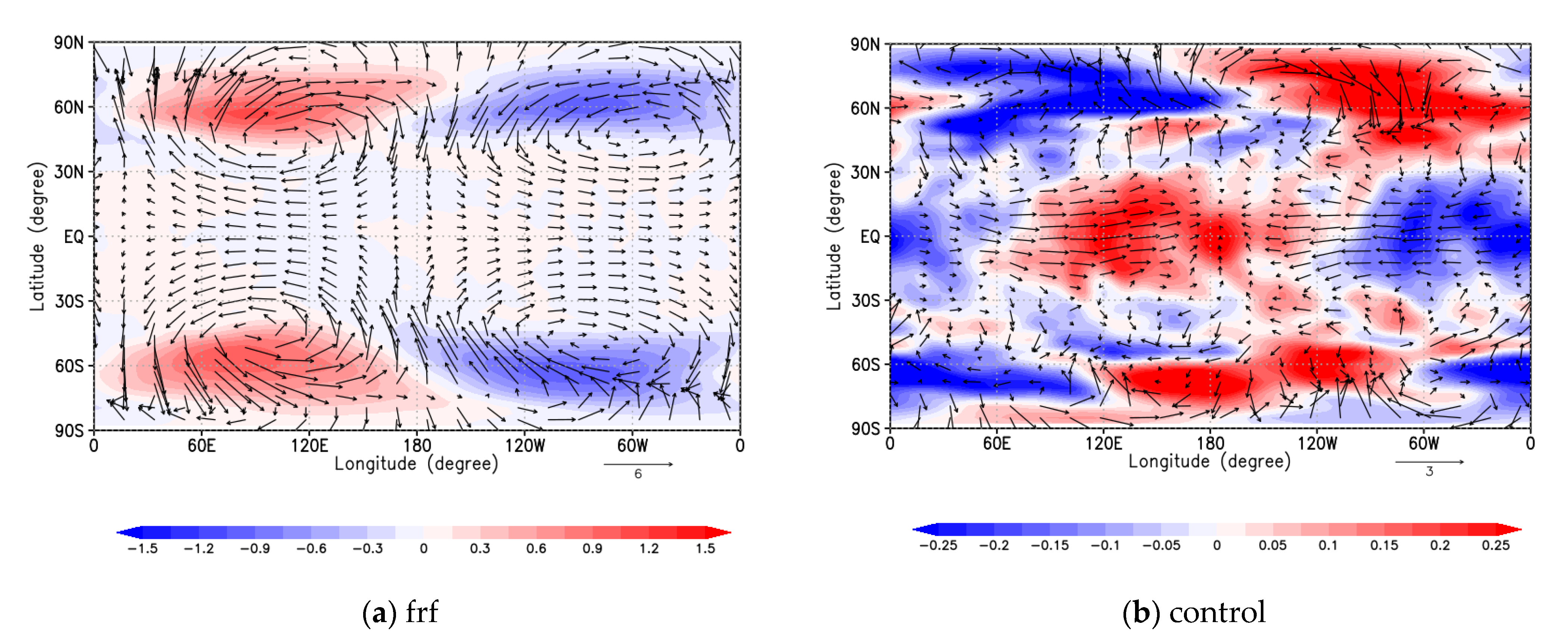
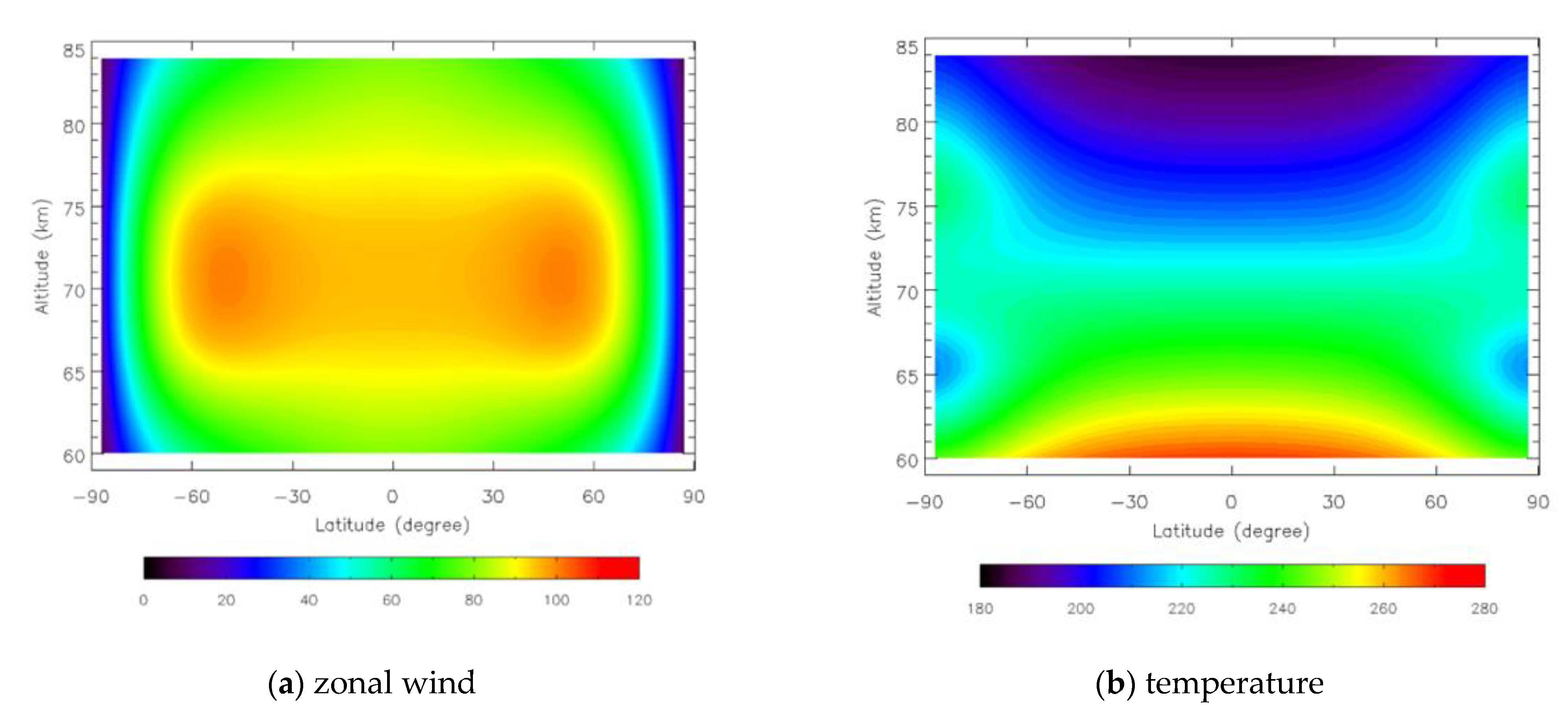
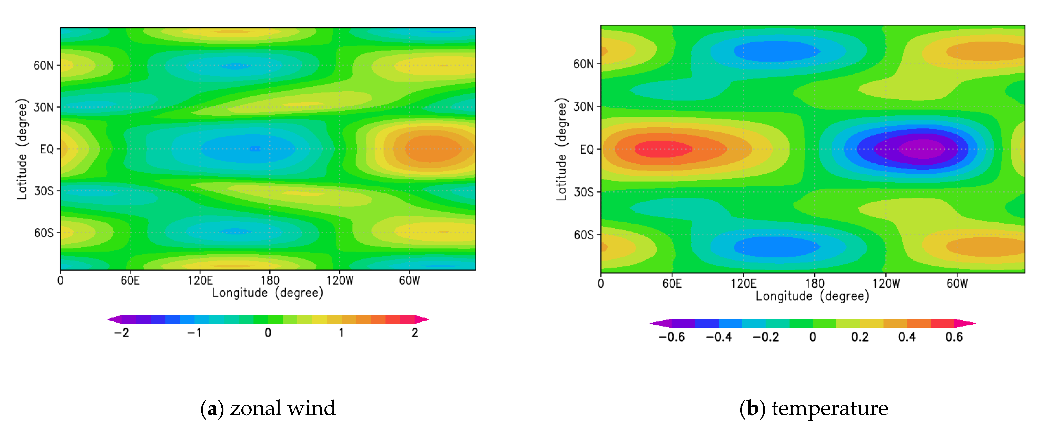
3.2. Composite Means

We extract wave structures by using composite methods, such as averaging each field with periods of 5 and 4 Earth days for the frf and control cases, respectively. Figure 4 shows the composite mean of horizontal wind sections (vector) and temperature (color) at 70 km for the (a) frf and (b) control cases. In the control case, zonal winds of ~2 m/s with a wavenumber 1 component symmetric around the equator prevail in the equatorial region, while meridional winds are small (Figure 4b). The Kelvin wave corresponds to this structure. The equatorial region similarly has a temperature of ~0.3 K with a wavenumber 1 component, although only horizontal winds are assimilated. The temperature phase differs by ~60° from the zonal wind phase, indicating that the wave propagates vertically [35].

The Rossby wave, on the other hand, appears in the frf case. In particular, vortices with a wavenumber 1 are predominant in the mid-latitudes, with zonal and meridional winds of ~5 m/s (Figure 4a). In the mid-to high-latitudes, a temperature of ~1.2 K with a wavenumber 1 component is also predominant. This structure is similar to the Rossby wave associated with baroclinic instability, as reported in a previous study [29]. It is worth noting that there is essentially no temperature disturbance in the equatorial region.

Figure 5 shows the composite mean of zonal wind in vertical sections at the equator for the (a) frf and (b) control cases. Again, the Kelvin wave is clearly reproduced only in the control case with both the zonal wind and temperature components. The Kelvin wave extends vertically for approximately 8 km (66–74 km altitudes), whereas horizontal winds are only assimilated at 70 km (Figure 5b; contour). It is worth noting that the vertical localization at 70 km is only ~O(10²) m, which is substantially less than the vertical grid interval of ~2 km. As a result, for dynamical reasons, the Kelvin wave would expand vertically. Temperature with a wavenumber 1 component predominates and has an inverted sign at an altitude of 70 km (Figure 5b; color). As in the horizontal structures, the temperature phase is 60° shifted from that of the zonal wind. The Kelvin wave appears to propagate vertically in both the zonal wind and temperature fields.

In contrast, the Rossby wave associated with baroclinic instability generated around 60 km is predominant for the frf case (Figure 5a). Above ~67 km, temperature disturbances are almost non-existent. While the large differences between the two cases are mostly caused by the composite means, the results suggest that the Kelvin wave reproduced by the horizontal wind assimilation would have a significant impact on the general circulation. We will investigate this in the next section.

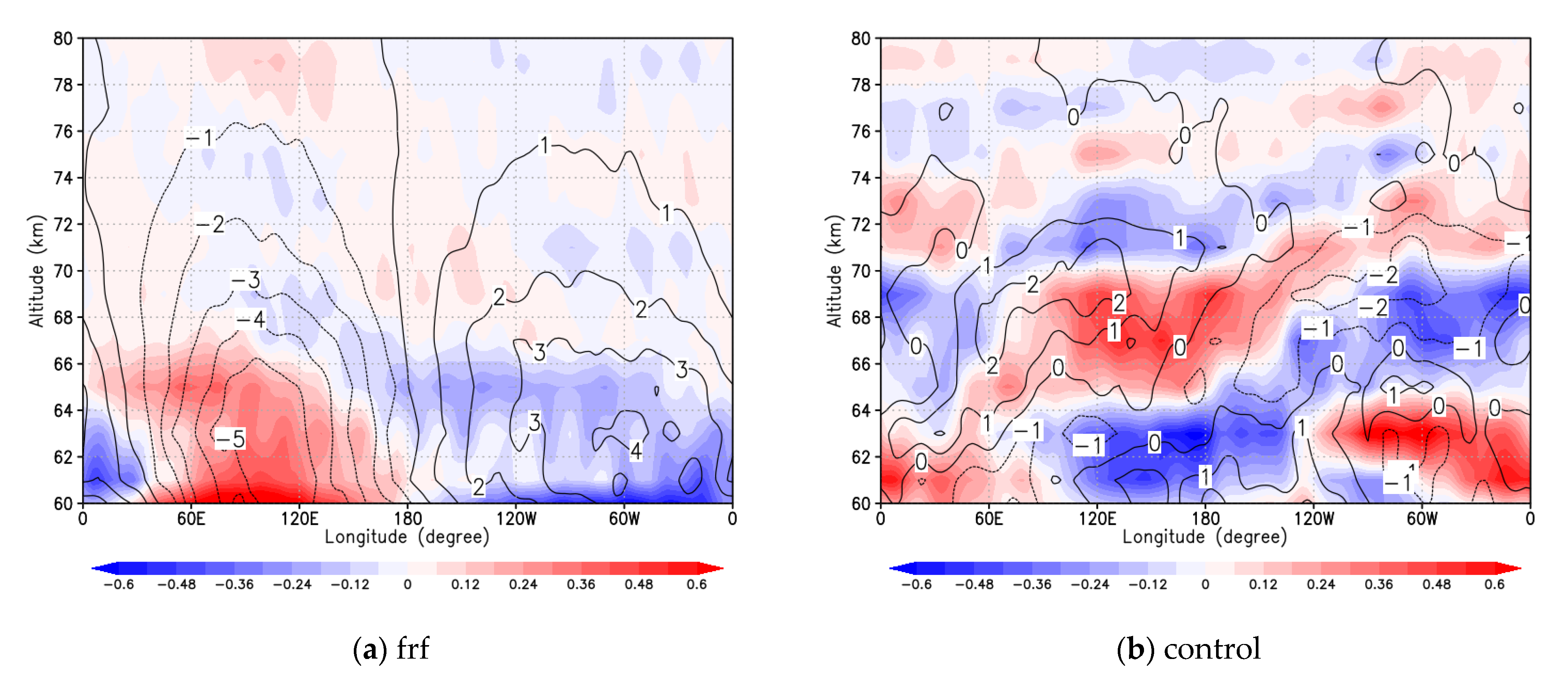
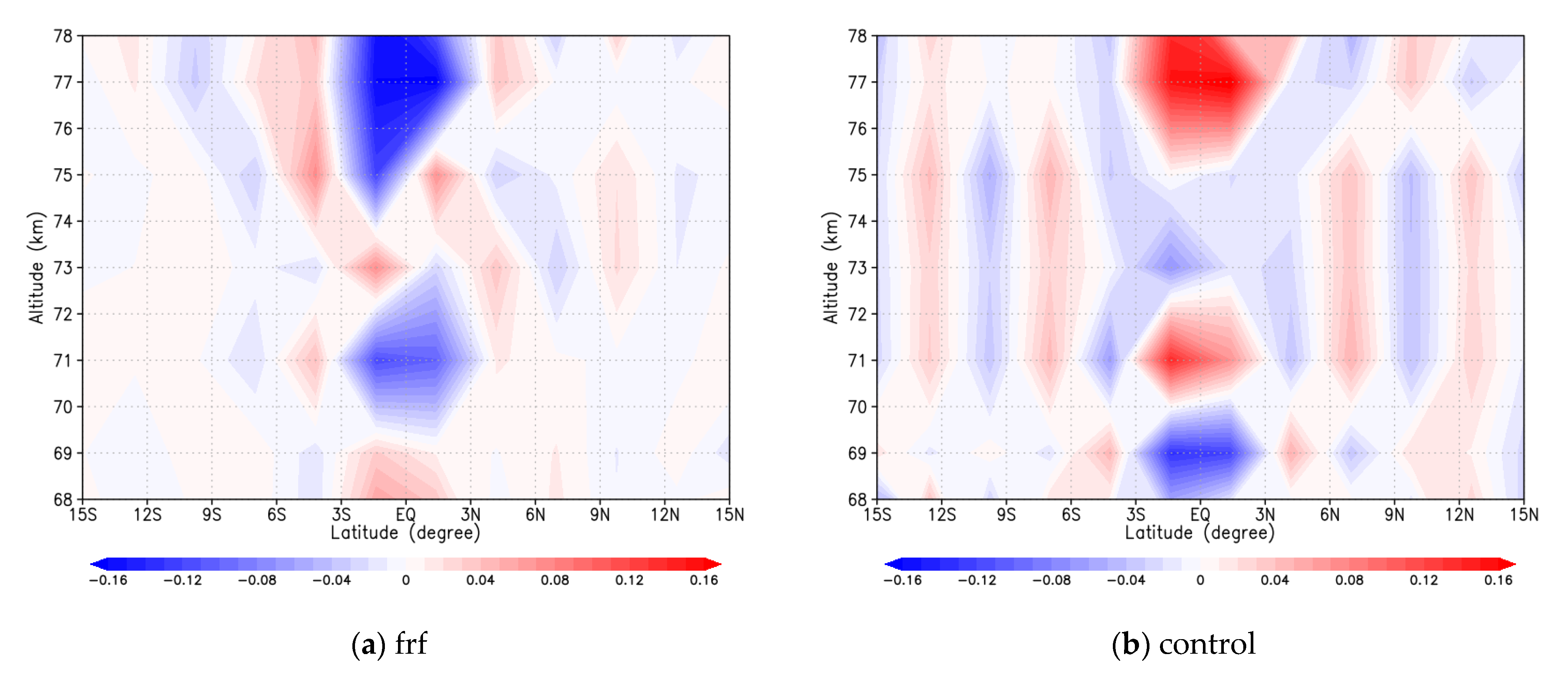
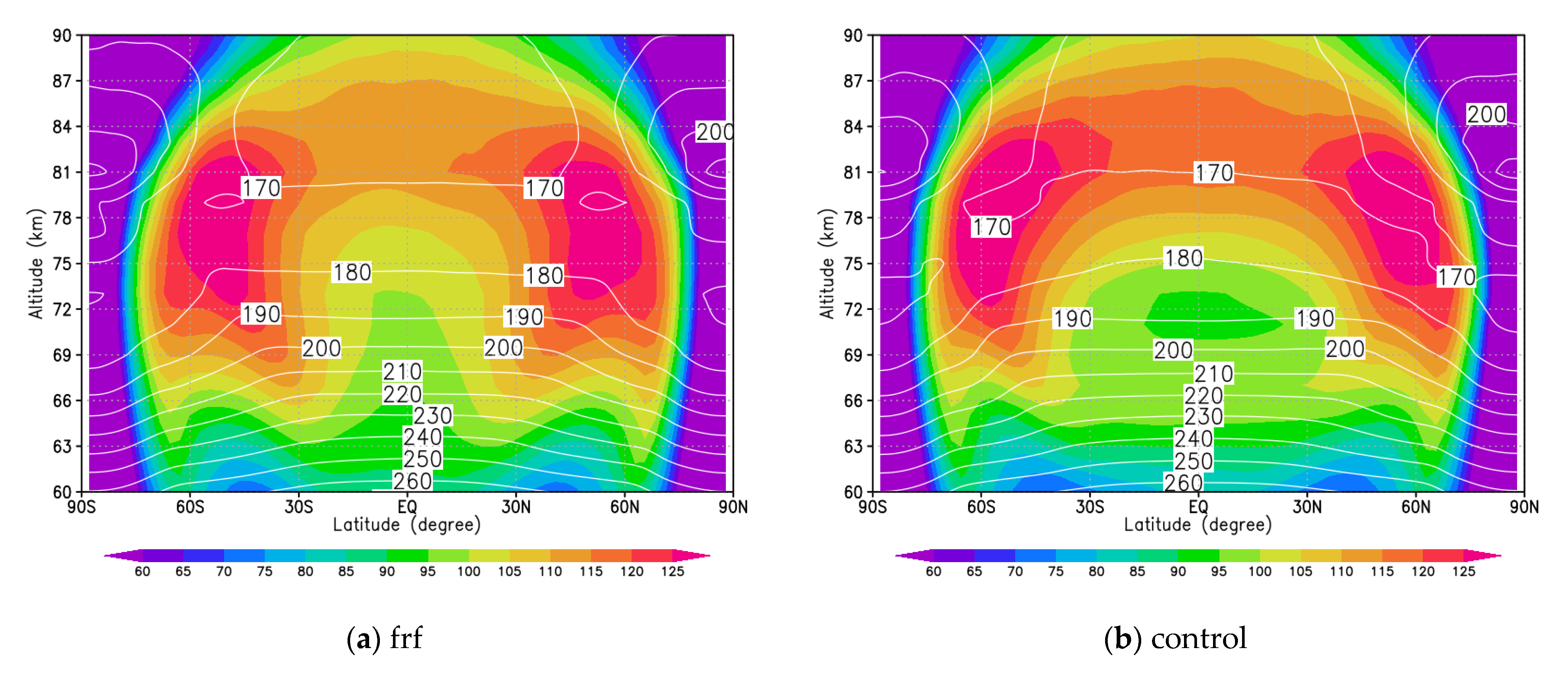
3.3. Impact of Kelvin Wave

We expect that the vertically propagating Kelvin wave transports angler momentum. To estimate wave-induced mean zonal wind accelerations, we evaluate the Eliassen–Palm (EP) fluxes [36,37] associated with waves. The EP flux vector $\overrightarrow{F}=\left(F^{\phi },F^z\right)$ is defined by

$$F^{\phi }={\rho }_0{R}_V\cos \phi \left(\frac{\partial \overline{u}}{\partial z^{*}}\frac{\overline{v^{\prime }{\theta }^{\prime }}}{\frac{\partial \overline{\theta }}{\partial z^{*}}}-\overline{u^{\prime }{v}^{\prime }}\right),$$

(1)

$$F^z=H{\rho }_0{R}_V\cos \phi \left\{\left[f-\frac{1}{R_V\cos \phi }\frac{\partial }{\partial \phi }\left(\overline{u}\cos \phi \right)\right]\frac{\overline{v^{\prime }{\theta }^{\prime }}}{\frac{\partial \overline{\theta }}{\partial z^{*}}}-\overline{u^{\prime }{w}^{\prime }}\right\},$$

(2)

where overbar and prime denote the zonal average and its deviation, respectively, and u, v, w, and θ represent the zonal, meridional, and vertical winds, and potential temperature, respectively. R_V and ${\rho }_0$ are the Venus radius and atmospheric density, respectively. $f=2\mathsf{\Omega }\sin \phi$ is the Coriolis parameter where $\mathsf{\Omega }$ and $\phi$ are the planetary rotational angular velocity and latitude, respectively. $z^{*}=–H \log \left(p/p_s\right)$ is a log-pressure height where H is the scale height, $p$ and $p_s$ are pressure and surface pressure, respectively. The wave-induced acceleration and deceleration of mean zonal wind is estimated by ${\left({\rho }_0{R}_V\cos \phi \right)}^{-1}\nabla ·\overrightarrow{F}$ with the EP flux divergence,

$$\nabla ·\overrightarrow{F}=\frac{1}{R_V\cos \phi }\frac{\partial }{\partial \phi }\left(F^{\phi }\cos \phi \right)+\frac{1}{H}\frac{\partial }{\partial z^{*}}\left(F^z\right),$$

(3)

Figure 6 shows latitude–altitude cross-sections of acceleration and deceleration estimated by the EP flux for the (a) frf and (b) control cases. Since there are many disturbances such as baroclinic (Rossby) and gravity waves in both experiments, the distributions of acceleration and deceleration associated with waves are complicated. Focusing on the equatorial region, while the Rossby wave mostly decelerates the mean zonal wind at 70–78 km altitudes (Figure 6a), the Kelvin wave accelerates it at these altitudes in the opposite sense (Figure 6b). It is worth noting that the Kelvin wave has a deceleration rate of ~0.1 m/s day⁻¹ when it is generated below 70 km and an acceleration rate of ~0.1 m/s day⁻¹ at 70–72 km altitudes. Then the Kelvin wave propagates vertically and accelerates mean zonal wind by ~0.1 m/s day⁻¹ above 75 km, which is consistent with previous estimates, e.g., [16]. This acceleration and deceleration will change the magnitude and structure of the super-rotation during the time evolution of OSSE.

Figure 7 shows latitude–altitude cross-sections of zonally averaged zonal wind (color) and temperature (contour). The generation of the Kelvin wave causes a deceleration of the super-rotation of ~5 m/s at ~70 km in the equatorial region. The Kelvin wave then accelerates the super-rotation by ~5 m/s at altitudes of 75–85 km between 45° S and 45° N. These accelerations and decelerations of the super-rotation are generated by a shift in the primary wave from the Rossby wave to the Kelvin wave, and are consistent with the EP flux estimations shown in Figure 6. The deceleration of roughly 70 km would also be caused by a somewhat slower super-rotation of the basic state used for synthetic observations (see Figure A1a). While OSSE is only performed for one Earth month in this study, the current result suggests that the Kelvin wave in the real Venus atmosphere can affect the magnitude of the super-rotation over a long period of time. It should be noted that zonally averaged zonal wind and temperature are produced by not only waves but the mean meridional circulation mainly generated by solar heating. Because the diurnal component of solar heating (and thus the thermal tide) is excluded in the present study in order to focus on the Kelvin wave, there are substantial mid-latitude jets (~125 m/s) in both present experiments when compared to real-world observations, e.g., [27,28].

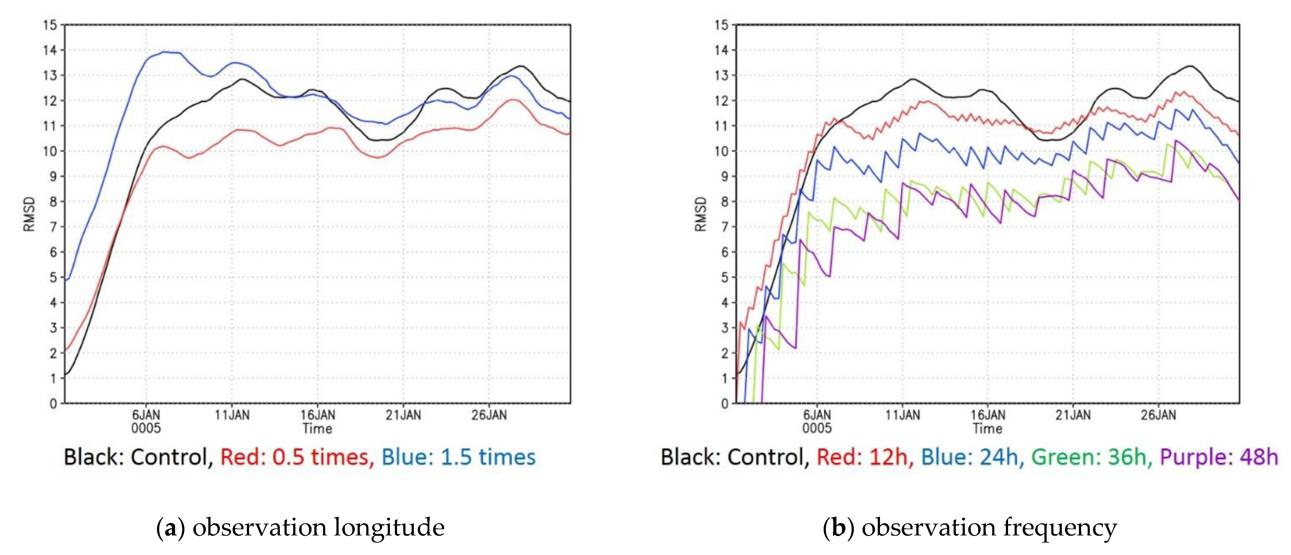
3.4. Requirements for Future Observations

Finally, we will investigate the conditions required to reproduce the Kelvin wave using actual data assimilation from satellite studies of horizontal winds, such as the Akatsuki Venus climate orbiter. On OSSEs, two types of sensitivity checks of synthetic observations were performed. The first is dependent on the range of observation longitude, and the second is dependent on observation frequency. To quantify the modification, we calculate the root-mean -square deviation (RMSD), which is defined as

$$RMSD=\sqrt{\frac{1}{N}{\displaystyle \sum }_{i=1}^N{\left(X_i-x_i\right)}^2},$$

(4)

where $X_i$ and $x_i$ indicate the results of the frf and each assimilated case, respectively, and N is the total number of horizontal grids at 70 km.

Figure 8 shows the time evolution of the RMSD for the sensitivity test of observation (a) longitude and (b) frequency. The dependence on the range of observation longitude is not as large in (a). If we can only observe half the zonal range compared to the control case (red line), the Kelvin wave is marginally reproduced. If the zonal range of observation is 1.5 times larger than the control case (blue line), improvement will be faster, but the final results will be almost unchanged. Figure 8b shows that the observation frequency is more important. For the cases of twice-a-day (12-Earth-hourly; red line) and once-a-day (24-Earth-hourly; blue line) observations, the Kelvin wave is marginally reproduced. The Kelvin wave, however, cannot be reproduced in other cases of 36-Earth-hourly (green line) and 48-Earth-hourly (purple line) observations. The RMSDs in these cases are kept at less than 10 most of the time, so enough modifications are not obtained by the data assimilation. It is worth noting that we also check horizontal structures in all cases to determine whether or not the Kelvin wave is reproduced (not shown). To duplicate the Kelvin wave, at least 24-hourly dayside observations will be needed, and if possible, 6-hourly would be preferable, even at the expense of a reduced observation range in longitude.

4. Summary

In this study, we performed OSSEs for the Venus atmosphere in order to reproduce the Kelvin wave using data assimilation, extending the previous study [12] in a more realistic way. The linear wave propagation model [15,16] with a basic state similar to that of AFES-Venus is used to generate synthetic observations of horizontal winds. In the control case, horizontal winds are assimilated at 70 km in 6-Earth-hourly intervals only on the dayside of the equatorial region, assuming cloud tracking of UVI is observed by satellites, such as the Akatsuki Venus climate orbiter. The Kelvin wave is then successfully reproduced not only in the zonal wind but also in temperature fields. It propagates vertically and transports angular momentum. We estimated the Eliassen–Palm (EP) fluxes and found that the Kelvin wave influences the magnitude and structure of the super-rotation through a ~0.1 m/s day⁻¹ acceleration and deceleration of zonal wind. To reproduce the Kelvin wave using horizontal wind assimilation, at least 24-hourly dayside satellite observations in the equatorial region are required, which may frequently be obtained using Akatsuki observations. As a result, if Akatsuki can study Venus at periods when the Kelvin wave appears for a period of several weeks, it is quite likely that we will reproduce the three-dimensional structure of the Kelvin wave by data assimilation and elucidate its impact on the super-rotation.

The latitudinal range of data assimilation was important in previous work because there is a large discrepancy between the basic states obtained by AFES-Venus and the CCSR/NIES (Center for Climate System Research/National Institute for Environmental Studies) Venus GCM [14], from which synthetic observations are produced. Since there are too strong mid-latitude jets at ~60° N (S) in the previous synthetic observations, OSSEs over larger latitudinal ranges did not always produce valuable results. Due to the similarity and consistency of the basic states, we do not require such a latitudinal restriction in this work. Because the Kelvin wave exists only in the equatorial zone, observations of the entire planet have less impact on the reproduction of the Kelvin wave (not shown) compared with the control case. To reproduce the Rossby wave in mid-latitudes and/or produce an objective analysis of the Venus atmosphere, the basic state of AFES-Venus must be consistent with observations over vast latitudinal ranges.

Previous research [3,38] suggested that the Rossby and Kelvin waves would induce super-rotation fluctuations over a long period of time. When the super-rotation is fast, the Rossby wave appears, but the Kelvin wave appears when the super-rotation is slow [16]. According to this study, the Kelvin wave causes an acceleration of ~0.1 m/s day⁻¹. The super-rotation would then fluctuate by O (10) m/s every 3 Earth months. In the future, we will use OSSEs to reproduce the Rossby wave and estimate its impact on the super-rotation. The observed long-term fluctuation of the super-rotation should be studied, with a focus on the momentum transport induced by both the Rossby and Kelvin waves. Finally, we emphasize that OSSEs would be valuable in designing missions not only for Venus but also for other planetary atmospheres.

References

1. Belton, M.J.S.; Smith, G.R.; Schubert, G.; Del Genio, A.D. Cloud patterns, waves and convection in the Venus atmosphere. J. Atmos. Sci. 1976, 33, 1394–1417. [Google Scholar] [CrossRef] [Green Version]
2. Del Genio, A.D.; Rossow, W.B. Planetary-scale waves and the cyclic nature of cloud top dynamics on Venus. J. Atmos. Sci. 1990, 47, 293–318. [Google Scholar] [CrossRef] [Green Version]
3. Khatuntsev, I.V.; Patsaeva, M.V.; Titov, D.V.; Ignatiev, N.I.; Turin, A.V.; Limaye, S.S.; Markiewicz, W.J.; Almeida, M.; Roatsch, T.; Moissl, R. Cloud level winds from the Venus Express Monitoring Camera imaging. Icarus 2013, 226, 140–158. [Google Scholar] [CrossRef]
4. Peralta, J.; Sánchez-Lavega, A.; López-Valverde, M.A.; Luz, D.; Machado, P. Venus’s major cloud feature as an equatorially trapped wave distorted by the wind. Geophys. Res. Lett. 2015, 42, 705–711. [Google Scholar] [CrossRef]
5. Sánchez-Lavega, A.; Lebonnois, S.; Imamura, T.; Read, P.L.; Luz, D. The Atmospheric Dynamics of Venus. Space Sci. Rev. 2017, 212, 1541–1616. [Google Scholar] [CrossRef]
6. Read, P.L.; Lebonnois, S. Superrotation on Venus, on Titan, and Elsewhere. Annu. Rev. Earth Planet. Sci. 2018, 46, 175–202. [Google Scholar] [CrossRef]
7. Kouyama, T.; Imamura, T.; Nakamura, M.; Satoh, T.; Futaana, Y. Horizontal structure of planetary-scale waves at the cloud top of Venus deduced from Galileo SSI images with an improved cloud-tracking technique. Planet. Space Sci. 2012, 60, 207–216. [Google Scholar] [CrossRef]
8. Imai, M.; Kouyama, T.; Takahashi, Y.; Yamazaki, A.; Watanabe, S.; Yamada, M.; Imamura, T.; Satoh, T.; Nakamura, M.; Murakami, S.; et al. Planetary-scale variations in winds and UV brightness at the Venusian cloud top: Periodicity and temporal evolution. J. Geophys. Res. Planets 2019, 124, 2635–2659. [Google Scholar] [CrossRef] [Green Version]
9. Miyoshi, T.; Yamane, S. Local ensemble transform Kalman filtering with an AGCM at a T159/L48 resolution. Mon. Weather. Rev. 2007, 135, 3841–3861. [Google Scholar] [CrossRef] [Green Version]
10. Sugimoto, N.; Takagi, M.; Matsuda, Y. Baroclinic instability in the Venus atmosphere simulated by GCM. J. Geophys. Res. 2014, 119, 1950–1968. [Google Scholar] [CrossRef]
11. Ohfuchi, W.; Nakamura, H.; Yoshioka, M.K.; Enomoto, T.; Takaya, K.; Peng, X.; Yamane, S.; Nishimura, T.; Kurihara, Y.; Ninomiya, K. 10-km Mesh Meso-scale Resolving Simulations of the Global Atmosphere on the Earth Simulator, -Preliminary Outcomes of AFES (AGCM for the Earth Simulator). J. Earth Simulator 2004, 1, 8–34. [Google Scholar]
12. Sugimoto, N.; Fujisawa, Y.; Shirasaka, M.; Hosono, A.; Abe, M.; Ando, H.; Takagi, M.; Yamamoto, M. Observing System Simulation Experiment to Reproduce Kelvin Wave in the Venus Atmosphere. Atmosphere 2021, 12, 14. [Google Scholar] [CrossRef]
13. Sugimoto, N.; Yamazaki, A.; Kouyama, T.; Kashimura, H.; Enomoto, T.; Takagi, M. Development of an ensemble Kalman filter data assimilation system for the Venusian atmosphere. Sci. Rep. 2017, 7, 9321. [Google Scholar] [CrossRef] [PubMed] [Green Version]
14. Yamamoto, M.; Takahashi, M. Venusian middle-atmospheric dynamics in the presence of a strong planetary-scale 5.5-day wave. Icarus 2012, 217, 702–713. [Google Scholar] [CrossRef]
15. Imamura, T. Meridional propagation of planetary-scale waves in vertical shear: Implication for the Venus atmosphere. J. Atmos. Sci. 2006, 63, 1623–1636. [Google Scholar] [CrossRef]
16. Kouyama, T.; Imamura, T.; Nakamura, M.; Satoh, T.; Futaana, Y. Vertical propagation of planetary-scale waves in variable background winds in the upper cloud region of Venus. Icarus 2015, 248, 560–568. [Google Scholar] [CrossRef]
17. Nakamura, M.; Imamura, T.; Ishii, N.; Abe, T.; Kawakatsu, Y.; Hirose, C.; Satoh, T.; Suzuki, M.; Ueno, M.; Yamazaki, A.; et al. AKATSUKI returns to Venus. Earth Planets Space 2016, 68, 75. [Google Scholar] [CrossRef] [Green Version]
18. Ikegawa, S.; Horinouchi, T. Improved automatic estimation of winds at the cloud top of Venus using superposition of cross-correlation surfaces. Icarus 2016, 271, 98–119. [Google Scholar] [CrossRef] [Green Version]
19. Sugimoto, N.; Kouyama, T.; Takagi, M. Impact of data assimilation on thermal tides in the case of Venus Express wind observation. Geophys. Res. Lett. 2019, 46, 4573–4580. [Google Scholar] [CrossRef]
20. Sugimoto, N.; Abe, M.; Kikuchi, Y.; Hosono, A.; Ando, H.; Takagi, M.; Garate-Lopez, I.; Lebonnois, S.; Ao, C. Observing system simulation experiment for radio occultation measurements of the Venus atmosphere among small satellites. J. Jpn. Soc. Civ. Eng. Ser. A2 (Appl. Mech.) 2019, 75, 477–486. [Google Scholar] [CrossRef]
21. Seiff, A.; Schofield, J.T.; Kliore, A.J.; Taylor, F.W.; Limaye, S.S.; Revercomb, H.E.; Sromovsky, L.A.; Kerzhanovich, V.V.; Moroz, V.I.; Marov, M.Y. Models of the structure of the atmosphere of Venus from the surface to 100 kilometers altitude. Adv. Space Res. 1985, 5, 3–58. [Google Scholar] [CrossRef]
22. Tomasko, M.G.; Doose, L.R.; Smith, P.H.; Odell, A.P. Measurements of the flux of sunlight in the atmosphere of Venus. J. Geophys. Res. 1980, 85, 8167–8186. [Google Scholar] [CrossRef]
23. Crisp, D. Radiative forcing of the Venus mesosphere: I. solar fluxes and heating rates. Icarus 1986, 67, 484–514. [Google Scholar] [CrossRef]
24. Lebonnois, S.; Sugimoto, N.; Gilli, G. Wave analysis in the atmosphere of Venus below 100-kmaltitude, simulated by the LMD Venus GCM. Icarus 2016, 278, 38–51. [Google Scholar] [CrossRef] [Green Version]
25. Yamamoto, M.; Ikeda, K.; Takahashi, M.; Horinouchi, T. Solar-locked and geographical atmospheric structures inferred from a Venus general circulation model with radiative transfer. Icarus 2019, 321, 232–250. [Google Scholar] [CrossRef]
26. Sugimoto, N.; Takagi, M.; Matsuda, Y. Fully developed super-rotation driven by the mean meridional circulation in a Venus GCM. Geophys. Res. Lett. 2019, 46, 1776–1784. [Google Scholar] [CrossRef]
27. Gorinov, D.A.; Zasova, L.V.; Khatuntsev, I.V.; Patsaeva, M.V.; Turin, A.V. Winds in the Lower Cloud Level on the Nightside of Venus from VIRTIS-M (Venus Express) 1.74 µm Images. Atmosphere 2021, 12, 186. [Google Scholar] [CrossRef]
28. Machado, P.; Widemann, T.; Peralta, J.; Gilli, G.; Espadinha, D.; Silva, J.E.; Brasil, F.; Ribeiro, J.; Gonçalves, R. Venus Atmospheric Dynamics at Two Altitudes: Akatsuki and Venus Express Cloud Tracking, Ground-Based Doppler Observations and Comparison with Modelling. Atmosphere 2021, 12, 506. [Google Scholar] [CrossRef]
29. Sugimoto, N.; Takagi, M.; Matsuda, Y. Waves in a Venus general circulation model. Geophys. Res. Lett. 2014, 41, 7461–7467. [Google Scholar] [CrossRef]
30. Ando, H.; Sugimoto, N.; Takagi, M.; Kashimura, H.; Imamura, T.; Matsuda, Y. The puzzling Venusian polar atmospheric structure reproduced by a general circulation model. Nat. Commun. 2016, 7, 10398. [Google Scholar] [CrossRef] [Green Version]
31. Takagi, M.; Sugimoto, N.; Ando, H.; Matsuda, Y. Three dimensional structures of thermal tides simulated by a Venus GCM. J. Geophys. Res. Planets 2018, 123, 335–352. [Google Scholar] [CrossRef]
32. Ando, H.; Takagi, M.; Fukuhara, T.; Imamura, T.; Sugimoto, N.; Sagawa, H.; Noguchi, K.; Tellmann, S.; Pätzold, M.; Häusler, B.; et al. Local time dependence of the thermal structure in the Venusian equatorial upper atmosphere: Comparison of Akatsuki radio occultation measurements and GCM results. J. Geophys. Res. Planets 2018, 123, 2970–2980. [Google Scholar] [CrossRef]
33. Kashimura, H.; Sugimoto, N.; Takagi, M.; Matsuda, Y.; Ohfuchi, W.; Enomoto, T.; Nakajima, K.; Ishiwatari, M.; Sato, T.M.; Hashimoto, G.L.; et al. Planetary-scale streak structure reproduced in a Venus atmospheric simulation. Nat. Commun. 2019, 10, 23. [Google Scholar] [CrossRef] [PubMed] [Green Version]
34. Sugimoto, N.; Fujisawa, Y.; Kashimura, H.; Noguchi, K.; Kuroda, T.; Takagi, M.; Hayashi, Y.Y. Generation of gravity waves from thermal tides in the Venus atmosphere. Nat. Commun. 2021, 12, 3682. [Google Scholar] [CrossRef] [PubMed]
35. Holton, J.R. An Introduction to Dyanamic Meteorology; Academic Press: Cambridge, MA, USA, 1992; Volume 48, pp. 1–511. [Google Scholar]
36. Andrews, D.G.; McIntyre, M.E. Planetary waves in horizontal and vertical shear: The generalized Eliassen-Palm relation and the mean zonal acceleration. J. Atmos. Sci. 1976, 33, 2031–2048. [Google Scholar] [CrossRef] [Green Version]
37. Andrews, D.G.; Holton, J.R.; Leovy, C.B. Middle Atmosphere Dynamics; Academic Press: Cambridge, MA, USA, 1987; Volume 40, pp. 1–489. [Google Scholar]
38. Kouyama, T.; Imamura, T.; Nakamura, M.; Satoh, T.; Futaana, Y. Long-term variation in the cloud-tracked zonal velocities at the cloud top of Venus deduced from Venus Express VMC images. J. Geophys. Res. 2013, 118, 37–46. [Google Scholar] [CrossRef]
Figure 1. Longitude–latitude cross-sections of horizontal winds (m/s; vector) and temperature (K; color) deviations from their zonal averages at 70 km for the control case.
Atmosphere 13 00182 g001
Figure 2. Longitude–time cross-sections of zonal wind (m/s) deviation from its time average from 1 January, 5th year at 70 km and the equator for the (a) frf and (b) control cases. Black arrows indicate periods of ~5 and ~4 Earth days for (a) and (b), respectively.
Atmosphere 13 00182 g002
Figure 3. Time-altitude cross-sections of zonal wind (m/s) deviation from its zonal and time averages at 10° W and the equator from 1 January, 5th year for the (a) frf and (b) control cases. Black lines indicate 70 km altitude.
Atmosphere 13 00182 g003
Figure 4. Longitude–latitude cross-sections of the composite means of horizontal wind (m/s; vector) and temperature (K; color) deviations from zonal averages at 70 km for the (a) frf and (b) control cases. Each field is averaged along with periods of 5 and 4 Earth days for the frf and control cases to extract the Rossby and Kelvin waves, respectively.
Atmosphere 13 00182 g004
Figure 5. Longitude–altitude cross-sections of composite means of zonal wind (m/s; contour) and temperature (K; color) deviations from their zonal averages at the equator for the (a) frf and (b) control cases. Each field is averaged along with periods of 5 and 4 Earth days for the frf and control cases to extract the Rossby and Kelvin waves, respectively.
Atmosphere 13 00182 g005
Figure 6. Latitude–altitude cross-sections of acceleration and deceleration (m/s day−1) estimated by the EP flux (color) for the (a) frf and (b) control cases. Time averages for 20 Earth days are conducted after the Kevin wave is reproduced.
Atmosphere 13 00182 g006
Figure 7. Latitude–altitude cross-sections of zonally averaged zonal wind (m/s; color) and temperature (K; contour) on 30 January, 5th year for the (a) frf and (b) control cases.
Atmosphere 13 00182 g007
Figure 8. Root-mean-square deviations (RMSD) of zonal wind (m/s) calculated by Equation (4) at 70 km in each assimilated case from 1 January, 5th year. Dependency on the range of (a) observation longitude and (b) observation frequency. In (a), observation longitudes are half (red line) and 1.5 times (blue line) of the control case with 120° (black line). In (b), observation frequencies are 12-Earth-hourly (red line), 24-Earth-hourly (blue line), 36-Earth-hourly (green line), and 48-Earth-hourly (purple line) compared with the control case with a 6-Earth-hourly (black line).
Atmosphere 13 00182 g008
Publisher’s Note: MDPI stays neutral with regard to jurisdictional claims in published maps and institutional affiliations.