Abstract
We present the results of observations of traveling ionospheric disturbances (TIDs) based on the data of the operation of the network of chirp oblique sounding stations of the ionosphere on 18–19 December 2019. For observations, four stations of the same type located in Vasilsursk (56.3° N; 46.08° E), Yoshkar-Ola (56.62° N; 47.87° E), Kazan (55.8° N; 49.12° E), and Nizhny Novgorod (56.32° N; 44.02° E) were used. They formed six synchronous sounding paths with lengths from 120 km to 320 km. The registration of the amplitude-frequency and distance-frequency characteristics (AFC and DFC) by the chirp oblique sounding stations was carried out every minute. Additionally, two vertical sounding stations of the ionosphere as ionosondes CADI and Cyclone (Vasilsursk and Kazan) were used. The passage of several types of TIDs has been observed. Based on the measurements of the DFC of the ionosphere, as obtained on different paths by simultaneously operated chirp stations, and ionograms obtained by vertical ionosondes, estimates of the spatial dimensions and TID velocity were made, and their direction was identified.
1. Introduction
Traveling ionospheric disturbances (TIDs) are typical ionospheric disturbances seen at mid-latitudes. They are wave-like propagating irregularities which are a manifestation of atmospheric gravity waves. For the first time, the observations of the TIDs were reported in 1940 by Pierce and Mimno [1]. Analysis of ionograms of the world network of ionosondes (ionospheric stations), working since the fifties of the last century, made it possible to obtain more information on the movements of ionospheric disturbances [2,3,4,5,6]. According to the classification accepted since the mid-sixties of the last century, TIDs are usually classified into three groups depending on their spatial scale. Large-scale TIDs have characteristic time from 0.5 to several hours and a spatial parameter up to several thousand kilometers; medium-scale TIDs have characteristic time of about several tens of minutes and a spatial parameter from one hundred to thousand kilometers; and small-scale TIDs keep a characteristic period of less than 10–15 min and the spatial one does not exceed 100 km (see, for examples [7,8]).
At the end of the 1990s, TIDs were classified depending on their wave velocity and period [7,9]. Fluctuating periods from 50 min to 3 h and horizontal velocities between 400 and 1000 m s−1 belong to large-scale TIDs, and horizontal velocities between 100 and 250 m s−1 and periods in the range of 15–60 min belong to medium-scale TIDs.
The development of shortwave communication facilities in the first half of the last century has become the reason for the active study of the ionosphere as a medium for propagation of radio waves. The relevance of TID studies is determined by their belonging to a wide class of ionospheric irregularities that affect communication in the shortwave (high frequency—HF) range.
Emergence of TIDs, for example, reduces the efficiency of the functioning of electronic systems for various purposes, causing a signal delay. Doppler amplification, signal build-up, and positioning errors can be detected, which are limiting factors for the development of modern communications, ultra-horizontal radars, and navigation aids.
The need to solve the inverse problem of remote sensing of the ionosphere requires clarifying the nature of wave disturbances and identifying their sources. For this, it is necessary to know the scale of wave disturbances, their dynamics during the time of their existence. Obtaining this information is possible only because of long-term complex experimental studies, which make it possible to carry out regular measurements of the most complete number of parameters of wave disturbances. However, it is extremely hard to interpret the observational results if the TIDs registered.
Currently, the IRI predictive reference model of the ionosphere [10] is widely used in calculations of radio wave propagation in the ionosphere.
Daily significant variations in ionospheric parameters, their strong dependence on heliogeophysical conditions, and the presence of parameters of traveling ionospheric disturbances of various scales that are poorly predicted in real conditions can negate the effectiveness of such a prediction. In this regard, the results of regular TID observations using networks of synchronously operating stations play a significant role, for example, by the oblique sounding method [11,12,13,14,15].
The most common way to study TIDs is to measure the altitude-frequency characteristics at ionospheric stations. In recent years, a variety of ground-based and space-based methods have been used for a detailed study of the parameters of TIDs traveling ionospheric disturbances: a network of synchronously operating HF DPS4D ionosondes, Doppler measurements, the GNSS TEC gradient method, spatial-temporal analysis of GPS satellite signals, short-wave interferometry, etc. All of them were actively used within a unified approach of European program TechTIDE project (Warning and Mitigation Technologies for Travelling Ionospheric Disturbances Effects—TechTIDE) [16].
Many articles and monographs are devoted to the analysis of TIDs behavior, their morphology, and connections with various geophysical phenomena (see, for example, [7,9,12,16,17,18,19,20,21,22] and the literature cited there).
The most significant advances have been made by Australian researchers from the Defense Science and Technology Group (Edinburgh, South Australia, Australia) [23] (see, for example, [14,15,24]), and they continue to study TIDs especially actively. Several groups of scientists in Russia are actively involved in research on TIDs: we have to mention the Institute of Solar-Terrestrial Physics of Siberian Branch of Russian Academy of Sciences (ISTP SB RAS), Radiophysical Research Institute Nizhny Novgorod State University (NIRFI), Pushkov Institute of Terrestrial Magnetism, Ionosphere and Radio-Wave Propagation Russian Academy of Sciences (IZMIRAN), and Federal State Autonomous Educational Institution of Higher Learning “Kazan (Volga Region) Federal University” (Kazan Federal University).
Pilot experiments on the generation of artificial TIDs were carried out by exposure to the ionosphere by high-power shortwave radiation using heating facilities: Universal Stand for Researching Near-Earth and Outer Space (SURA facility, Russia, NIRFI)) and High-frequency Active Auroral Research Program (HAARP, USA, the University of Alaska Fairbanks) [17,25,26].
Some authors [27,28,29,30] have proposed mechanisms to explain the generation of internal waves, including cases when the ionosphere is modified by powerful radio waves.
Let us pay attention to one of the most interesting manifestations of TIDs at mid-latitudes: crescent (U-shaped) tracks on ionogram of vertical and slightly oblique sounding methods of ionospheric research. U-shaped tracks are seen in ionograms just near the region of critical frequencies and usually move from high altitudes to lower ones in no more than 15 min.
Such manifestations are usually observed on 1–2 adjacent ionograms and look like a sudden added increase in the electron concentration at the heights of the F-layer of the ionosphere, moving towards the base of the layer. We find it so because of the standard fifteen-minute mode of ionograms recording by ionosondes of the world network of ionospheric stations.
A detailed analysis of the occurrence of such sickle shaped TIDs at mid-latitudes for several cycles of solar activity was carried out using data from Zimenki station (Nizhny Novgorod) [17]. It was shown that this is a typical daytime phenomenon, depending on helio geomagnetic activity in a complex way.
This article presents the results of a special experiment on the registration of traveling ionospheric disturbances by a system of synchronously operating chirp ionosondes located in the city of Nizhny Novgorod, Vasilsursk village (NIRFI), the city of Yoshkar-Ola (Sitcom LLT), and the city of Kazan (KFU), with weakly inclined sounding of the ionosphere during the passage of traveling ionospheric disturbances of the sickle type.
2. Materials and Methods
2.1. Location (Experiment Geometry) and Method
The experiment was conducted by scientists of Radiophysical Research Institute Lobachevsky State University of Nizhny Novgorod, Kazan (Volga region) Federal University, and “SITCOM” LLC, Yoshkar-Ola, Russia. All participants in the experiment had experience with chirp equipment.
Observations were carried out on 18–19 December 2019. According to earlier studies [17], where it was shown that sickle shaped TIDs are the typical daytime phenomenon, the operating time was determined by the highest probability of observing TIDs at middle latitudes from 11:30 to 13:30 Moscow time.
As mentioned above, for the reliable registration of TIDs, it is important to be able to use the network of chirp stations continuously for several hours. Therefore, it was decided to use a sequential radiation regime for each participant in the experiment.
The work schedule of chirp stations for transmission is cyclical in the following order: the zero min corresponds to Yoshkar-Ola, the first min—to Kazan, the second min—to Vasilsursk, etc. Thus, the program repeatability was 3 min, and a frequency tuning rate of 110 kHz/s was used. The starting frequency was 3 MHz, and the ending frequency was 9 MHz on 18 December and 8.5 MHz on 19 December 2019. When the chirp station does not work on transmission, it receives the chirp signal reflected from the ionosphere. The station in Nizhny Novgorod city has been used as receiving station only. The chirp station of IZMIRAN was independently used for receiving the signal on 19 December 2019.
The geometry of the paths’ network for diagnosing the ionosphere using chirp signals is shown in Figure 1. White dots in the figure mark the locations of chirp stations: receiving and transmitting in the village of Vasilsursk, Kazan, and Yoshkar-Ola cities; receiving station in Nizhny Novgorod city.
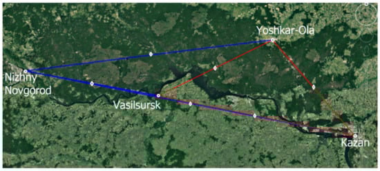
Figure 1.
Paths’ network for diagnosing the ionosphere using chirp signals.
The red lines mark the paths where the chirp stations worked as receiving and transmitting; blue lines mean receiving only. The midpoints of the sounding paths are marked by white diamonds. The coordinates of the chirp stations are shown in Table 1. The R or T symbols in the Table 1 mark the chirp stations, working for reception or transmission, respectively.

Table 1.
Coordinates of chirp stations.
As seen in Figure 1, the actual number of possible sounding tracks was six. Their parameters are given in Table 2.
Table 2.
Sounding paths parameters.
2.2. Equipment Used
All used chirp stations were designed and manufactured by SITCOM LLC, Yoshkar-Ola. The central station was installed in Vasilsursk and included an IC1000 power amplifier (Figure 2).
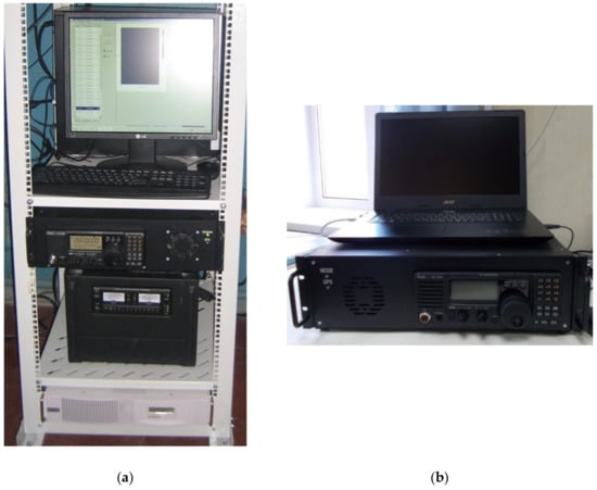
Figure 2.
(a) LFM station in Vasilsursk; (b) LFM station at other points.
Unfortunately, during the experiment, the used antennas at the chirp points were not the same, and their parameters differed quite strongly. It was so because of the peculiarities of the chirp station’s location.
So, in the village Vasilsursk the antenna was a vertical Delta located on the 40-m mast (Figure 3).
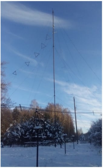
Figure 3.
Antenna in village Vasilsursk: vertical Delta located on the 40-m mast.
The same vertical Delta antenna was used in Nizhny Novgorod city but located on 15-m mast. A 40-m oblique beam steered from the roof of a highest building of the Physics Faculty of Kazan Federal University was used as antenna for chirp station in Kazan. The antenna in Yoshkar-Ola chirp point was represented as T2FD antenna. The antenna parameters in the village Vasilsursk did not allow for radiation of more than 300 W. The maximum output power in the chirp radiate mode in Kazan and Yoshkar-Ola was no more than 100 W.
Additionally, two vertical sounding ionosonde worked during the experiment: Canadian Advanced Digital Ionosonde (CADI) [31] in Vasilsursk, and the Cyclone [32] ionosonde near Kazan. The working program of regular observations using CADI, allowed researchers to obtain ionograms at least once every 15 min, while the usage of the Cyclone allowed researchers to obtain ionograms at least once every 1 min.
3. Results
During the experiment, records of distance-frequency characteristics (DFC) were obtained in the mode of weakly oblique sounding of the ionosphere along different paths by four operated ionosondes. The critical frequencies of the ionosphere were found using CADI ionosonde data. Sickle-shaped TIDs of various configurations were observed.
The emergence of disturbances was accompanied by a loop distortion of the ionogram in the critical frequency range of the F-region of the ionosphere. Then an inflection occurred, which shifted to the low-frequency part of the ionogram along the O- or X-track axis. These are the so-called sickle-shaped disturbances.
An example of a sickle-shaped TID at the distance-frequency characteristic is shown in Figure 4 for the Vasilsursk-Kazan path on 18 December 2019, at 09:56 UT. TID is also seen at the second jump in the DFC, with the reflection tracks being diffuse.
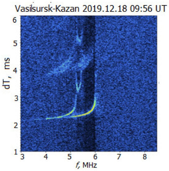
Figure 4.
An example of a sickle-shaped TID for the Vasilsursk-Kazan path on 18 December 2019.
Note that on 18 December 2019, from 09:13 to 09:17 UT, a TID was registered on the Yoshkar-Ola—Kazan path and was not recorded on the other paths. Considering the distance between the midpoints of the paths, it can be assumed that the specific horizontal dimensions of such ionospheric disturbance did not exceed 100 km.
Strong ionospheric disturbances were detected on 19 December 2019 (see, for example, Figure 5).
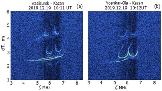
Figure 5.
RFC recorded on 19 December 2019. (a) Vasilsursk-Kazan path, 10:11 UT; (b) Yoshkar-Ola-Kazan path, 10:12 UT.
Sickle-shaped TIDs were recorded multiple times on all sounding paths. The frequency range of the TID reached 0.8 MHz, while the critical frequencies of F-layer were about 6 MHz.
The observed TID structure resembled that previously discussed in [33]. The authors have determined the directional-velocity characteristics of medium scale TID by comparing the experimental and calculated TID by the method of numerical modeling of ionograms of quasi-vertical ionospheric sounding. The obtained values of the directional-velocity characteristics are in good agreement with the time evolution of the response of the broadband signal to the passage of the wave disturbance along the sounding path.
It should be noted that it was previously believed that mid-latitude TIDs have a phase movement exclusively from high altitudes to lower ones. We have never observed the phases of the return TID movements from low altitudes to higher ones. Figure 6 shows a set of ionograms illustrating these processes.
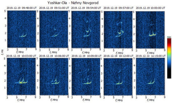
Figure 6.
Illustration of the TID movement “top-down” (upper panel) and “bottom-up”(low panel) on the Yoshkar-Ola-Vasilsursk path.
The method of the maximum of the cross-correlation function and the “phase front” method, proposed in [6], were used to determine the direction in the space of the ionospheric disturbance front movement for the case of simultaneous registration of TIDs on several sounding paths (the front is supposed to be plane).
3.1. Determination Parameters of TID Movement
To figure out the parameters of TID movement we used three paths for calculation: Kazan-Yoshkar-Ola (length 120 km, azimuth 319.5°), Vasilsursk-Yoshkar-Ola (length 123 km, azimuth 64°), and Kazan-Vasilsursk (length 192 km, azimuth 281°). The rest of the paths (Vasilsursk-Nizhny Novgorod and Yoshkar-Ola-Nizhny Novgorod) were made use of as the control. The paths Vasilsursk-Yoshkar-Ola and Kazan-Yoshkar-Ola were used to determine the direction of TIDs.
The total power of the TID signal received in the recording band, normalized to the average noise power, was used as a numerical measure of the DFC disturbance. Ionograms are presented in Figure 7 with inverted colors for readability. Figure 7a,b show the same shaped but time-shifted changes in TIDs. Sickle shaped TIDs were recorded first on Vasilsursk-Yoshkar-Ola path, and then in 8 min later Kazan-Yoshkar-Ola path. The tracks of TIDs are marked with circles on the top panels of Figure 7.
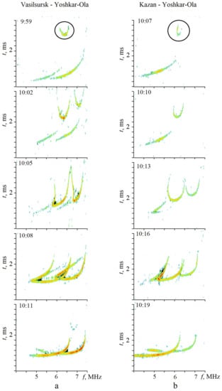
Figure 7.
Ionograms for Vasilsursk-Yoshkar-Ola (a) and Kazan-Yoshkar-Ola (b) on 19 December 2019.
To estimate the time lag between the signals, the cross-correlation functions were determined, and their maxima were found.
The results of measurements which are normalized to the maximum value of TID signal power (Anorm) on 19 December are shown in Figure 8. The observational time was from 9:30 to 10:30 UT on the paths Vasilsursk-Yoshkar-Ola, Kazan-Yoshkar-Ola, and Kazan-Vasilsursk.
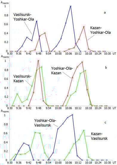
Figure 8.
Results of measurements the normalized values of TID signal power on 19 December 2019, during time from 9:30 to 10:30 UT on the paths Vasilsursk-Yoshkar-Ola (a,c), Kazan-Yoshkar-Ola (a,b), and Kazan-Vasilsursk (b,c).
The graphs are built separately for forward and backward sounding traces with measured values. The listing begins from the transmitting chirp station to the receiving station. As we can see on the Figure 8, forward and backward sounding traces are marked by the same color: Kazan-Yoshkar-Ola (Figure 8a) and Yoshkar-Ola-Kazan (Figure 8b) paths are shown as red solid line and red crosses; Vasilsursk-Yoshkar-Ola (Figure 8a) and Yoshkar-Ola-Vasilsursk(Figure 8c) paths are shown as blue solid line and blue crosses, and Vasilsursk-Kazan (Figure 8b) and Kazan-Vasilsursk(Figure 8c) paths are denoted as green solid line and green crosses.
Two TIDs were seen on all paths during the above mentioned period: on 19 December 2019, from 9:30 to 10:30 UT.
Table 3 shows the TID time interval between the various paths, the distance between the midpoints of the paths, and the initial azimuth from the midpoint of the first path to the midpoint of the second path in the direction of the disturbance. The sign minus means that the disturbance propagates in the direction from the middle of the second path to the middle of the first path.
Table 3.
Time delay of TID.
Using the data in Table 3, we will determine the direction and speed of the TIDs.
Let us denote l—distance, α—azimuth, t—time delay of TID between midpoints of paths, υ is the modulus, and φ is the azimuth of the disturbance velocity vector; then, we can find the modulus of the velocity and the direction of motion of the disturbance.
Let i = 1 be the index of the midpoint of Kazan-Yoshkar-Ola path, i = 2 be the index of Vasilsursk-Yoshkar-Ola path, and i = 3 be the index of Kazan-Vasilsursk path. Then three variants of systems of equations are possible, differing in indices:
v·t1i = l1i·cos(α1i – φ), i = 2, 3;
v·t2i = l2i·cos(α2i – φ), i = 2, 3.
The solution of the first system gives the following values for the modulus of the disturbance: velocity vector v = 120 m/s and the azimuth of the velocity vector φ = 154°; solution of the second system gives v = 100 m/s and φ = 161°; and the third system solution gives v = 115 m/s and φ = 161°. The average value of the velocity of the ionospheric disturbance is defined as 111.7 m/s with a standard deviation of 8.5 m/s, and the average value of the azimuth is 158.7° with a standard deviation of 3.3°. Note that when three different options for radio paths were selected, similar numerical results were obtained for the magnitude and direction of the TID velocity vector.
Knowing the velocity vector of the disturbance and the duration of its effect on the signal in each radio path, it is possible to estimate the size of the TID in the direction of its movement. For the Yoshkar-Ola-Vasilsursk path, the durations of the TID passages are 420 s and 690 s (at the level of 0.5 in Figure 8). It corresponds to the dimensions of 47 and 77 km, respectively for a speed of 111.7 m/s.
The control of the Vasilsursk-Nizhny Novgorod (registration time 10:04–10:16 UT) and Yoshkar-Ola-Nizhny Novgorod (registration time 9:51–10:12 UT) paths convinces into the rightness of the obtained velocity and direction values, and confirms the correctness of the assumption about the plane front of the ionospheric disturbance within a distance along the front of about 130 km.
The only exception is the Vasilsursk-Nizhny Novgorod path, where the TID is seen a minute earlier than for the Yoshkar-Ola-Nizhny Novgorod paths and quite well coincides in the dynamics of changes on this path (see Figure 6). Probably, the same features of these paths may indicate a possible additional disturbance of the ionosphere from the west.
Application of the phase front method [6] to determine the parameters of the TID in this experiment is limited by the features of the geometry of the paths and the horizontal speed of the TID.
The midpoints of the Yoshkar-Ola-Nizhny Novgorod, Yoshkar-Ola-Vasilsursk, and Yoshkar-Ola-Kazan paths were located almost on the same line: the distance between the midpoint of the Yoshkar-Ola-Vasilsursk path and the line connecting the midpoints of the other two paths is 2 km. Under such conditions, only estimates of the TID vertical velocity were carried out.
For this purpose, plasma frequencies of the intersection the points of the TID tracks and the regular track of the F-layer were found for three considered paths during the passage of the TID at times 8:39 and 8:42 UT [6].
For them, the true reflection heights were reconstructed considering the slope of the path. The changes in heights were determined in 3 min: for the Yoshkar-Ola-Nizhny Novgorod path it is 7.5 km (initial 190.5 and final 183.0 heights in km); for Yoshkar-Ola-Vasilsursk path it is 10.6 km (205.0 and 194.4 km, respectively), and for Yoshkar-Ola-Kazan path it is 10.8 km (196.0 and 185.2 km, respectively).
The average value of the vertical velocity of the TID was 53.5 m/s.
To calculate the true heights, we used the POLAN program in the Fortran language by J.E. Titheridge [34]. Review of all possible combinations of paths showed that the phase front method is not applicable under the conditions of this experiment due to the velocity parameters of the TID, the direction of motion, the duration of the disturbance, the geometry of the experiment, and the difficulties in interpreting the DFC. E. Titheridge’s method is described in detail in [35].
It should be noted that TIDs were also observed on 18 December 2019, within the framework of this experiment. But their number and intensity were significantly inferior to the observed ones on 19 December. That is why the focus of this work is on the ionosphere of 19 December 2019.
3.2. The State of the Daytime Ionosphere on 19 December 2019 (According to the CADI Ionosonde in Vasilsursk)
The CADI ionosonde was installed at the Vasilsursk test site in 2012. Since 1 January 2013, it has been working in the mode of patrol observations and accompaniment of experimental research during the operation of the SURA heating facility.
During this special experiment, the CADI ionosonde operated in the usual 15-min mode of recording ionograms of vertical sounding of the ionosphere. It was impossible to switch it to the minute mode, because in this case, it would interfere with receiving signals from chirp stations.
Nevertheless, ionosonde data were used both for operational monitoring of the state of the ionosphere and for analyzing the time variation of the critical frequency of the F-layer of the ionosphere F2.
Figure 9 shows the graphs of the critical frequency F2 behavior and the true reflection height h in time for the period from 6 to 11 UT. The graphs are supplemented with approximation curves with polynomial dependence of the 2nd (critical frequency) and the 4th (true reflection height) orders.
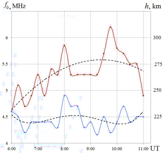
Figure 9.
Dependence of the critical frequency f0 of the ionosphere (red) and true reflection height h at a frequency of 4 MHz (blue) according to the CADI ionosonde (Vasilsursk) on 19 December 2019. Approximation lines are drawn by a dotted line.
Changes in the critical frequency by 0.5–1.0 MHz are clearly visible with periods of 0.5–1.5 h and more. The deviations of the true heights at a frequency of 4 MHz were up to 20 km from the average value of 225 km with characteristic periods of 0.5–4 h. The presence of periodic variations in the criterion frequency and reflection heights for the F-layer of the ionosphere is noted as an indispensable feature in the registration of TID [7].
4. Discussion
Planning this experiment, we took into account the well-known results of analysis of the data of vertical ionospheric sounding during several cycles of solar activity [17]. The distinctive feature of this study was the following: there was the registration of the appearance of sickle-like TIDs during all studied solar cycles (in January), and the maximum of the cases seen corresponds to the near-midday time. In addition, the maximum frequency of this type events is observed with a decrease or increase in solar activity.
We have considered the recommendations for the choice of the length of the paths [14]. The possibility of observations along long paths is realized using the receiving chirp station in Nizhny Novgorod. The results obtained in Troitsk (IZMIRAN) on an independent path 400–500 km long are not discussed here because of the need for added processing.
Note that during the experiment, the CADI ionosonde in Vasilsursk was constantly operating in the 15-min sounding mode, and occasionally in the one-minute sounding mode the Cyclone ionosonde was working.
The data of these two ionosondes were used to reconstruct the altitude profile of the electron density and observed variations in the critical frequency and operating altitude at a frequency of 4 MHz.
A comparative analysis of ionograms of vertical and oblique sounding of the ionosphere obtained during the experiment showed that the chirp stations (with approximately the same equivalent technical parameters) make it possible to record TIDs of the sickle-type more efficiently.
Note, the CADI ionosonde did not record the passage of the TID on 18 December 2019. Only weak diffuseness of 1–2 points [35] was seen on ionograms up to 9:45 inclusive. At the same time, sickle-type TIDs were observed on 18 December in three ionograms on the paths Kazan-Nizhny Novgorod (with the midpoint of the path closest to Vasilsursk) and Vasilsursk-Nizhny Novgorod.
On 19 December, the CADI ionosonde recorded the sickle-type TIDs three times: 8:45, 10:00, and 10:15 UT, but more disturbances were recorded, and they were significantly longer on chirp paths Kazan-Nizhny Novgorod and Vasilsursk-Nizhny Novgorod. For the path Kazan-Nizhny Novgorod, one can see the sickle TIDs from 8:31 to 20:46, from 9:01 to 9:10, at 9:22, from 9:34 to 9:52, and from 10:04 to 10:16 UT. For the path Vasilsursk-Nizhny Novgorod, there were recorded the sickle-type TIDs from 8: 32 to 8:47, from 8:53 to 9:02 a.m., at 9:17 a.m., from 9:50 a.m. to 10:08 a.m., and at 10:29 a.m. UT.
We unambiguously associate the increase in the number of disturbances on 19 December relative to 18 December with the dynamics of helio activity.
The Sun can be considered very calm in the period of December 2019: not a single active region (AR) was observed until December 25, and even weak flares were not recorded in the two ARs that appeared later [36]. No changes were recorded in the X-ray radiation of the Sun, which characterize the flare activity (Figure 10). Small number of CME has been recorded by LASCO [37]. At the same time, on 18–19 December, the passage of a high-speed solar wind flux at a speed of about 550 km/s was recorded [38]. The geophysical environment on 18–19 December 2019 was quiet, as well (see Figure 10). The maximum value of the Dst index (18 nT) was registered on 18 December at 03:00 UT. The minimum values were observed on 18 December at 19:00 UT (−28 nT), and on 19 December at 13:00 UT (−26 nT) [39]. Such DST values are less than even those that describe moderate geomagnetic storms (below then −50 nT). The Kp index reached its maximum value of 4 on 18 December at 15:00 UT [40].
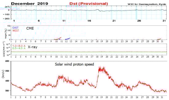
Figure 10.
Dynamics of helio geophysical activity in December 2019.
As we see from Figure 10, the experiment took place under conditions of minimum solar activity, when even weak manifestations of helio activity were not observed for a whole period examined. Only a sharp increase in the speed of the high-speed solar wind stream up to 550 km/s on 18–19 December led to an increase in ionospheric disturbances and influenced slightly on increase in geomagnetic activity (a decrease in the Dst index to −28 nT and an increase in the Kp index up to 4).
If we consider the recorded crescent traveling ionospheric disturbances as traveling wave packets (TWP) of total electron content (TEC) disturbances (similar to [41]), then there is a fairly good agreement between the conditions for their observation. Indeed, dependence of the number of TWPs on the modulus of the Dst-index less than 50 nT (in our case, from 18 to −28 nT); diurnal distribution of the times tmax corresponding to the maximum amplitude Amax of the wave packet of the TEC disturbance falls during 9–12 h LT (in our case, 11–13 h LT).
We believe that it is the wave processes in the upper ionosphere that are the cause of the observed sickle-type TIDs. The sources of these waves are located to the north of our station, according to a certain direction of wave propagation: they are generated in the auroral oval or terminator during geomagnetic disturbances [7]. In our opinion, when solving the inverse problem of remote sensing of the ionosphere during the passage of a wave disturbance, it is necessary to take into account the orientation of its wavefront along the lines of force of the geomagnetic field.
We did not conduct a separate analysis of the O- and X-components of disturbances in this article, leaving it for the next stage of study. We plan to fulfill ray modeling using both our processing programs and program of the Defense Science and Technology Organization (Edinburgh, Australia); it is posted on the website.
As an extension of this study, we propose to continue the comprehensive research of traveling ionospheric disturbances. We plan not only to increase the number of paths, but also to use the available methods of trans ionospheric sounding of the ionosphere by signals from artificial earth satellites in the mid-latitude ionosphere. Unfortunately, we cannot afford to conduct long-term observations (as it was in the case of TechTide and SpICE projects), because it is exceedingly difficult to organize extensive observations by scientists from different organizations located far from each other.
Nevertheless, in the fall of 2021, we already tried to work in a network of chirp stations with a successful TID registration. The results of this study will be reported later.
As we mentioned, there are known works on the generation of TID by high-power short-wave radiation from the SURA heating facility [17,25,26]. This work has not yet been completed. We hope to continue it for the study of sickle type TIDs.
5. Conclusions
This article presented the results of special experiment (on 18–19 December 2021) on the registration of traveling ionospheric disturbances by a system of synchronously operating chirp ionosondes located in the city of Nizhny Novgorod, Vasilsursk village (NIRFI), the city of Yoshkar-Ola (Sitcom LLT), and the city of Kazan (KFU). The purpose of this experiment was to register the propagation of traveling crescent-type ionospheric disturbances in the ionosphere. Strong ionospheric disturbances were detected on 19 December 2019. Sickle shaped TIDs were recorded multiple times on all sounding paths. The frequency range of the TID reached 0.8 MHz, while the critical frequencies of F-layer were about 6 MHz.
The previously established fact about the direction of TIDs movement was confirmed: mid-latitude TIDs have a phase of movement from high altitudes to lower ones. Additionally, we have seen the return TID movements from low altitudes to higher ones.
Sickle shaped TIDs were observed with the time lag between the signals from 1 to 8 min. Knowing time lag allowed us to determine the direction and speed of the TIDs. The average value of the velocity of the ionospheric disturbance is defined as 111.7 m/s, the average value of the azimuth is 158.7°, and the dimensions are 47 and 77 km. According to the generally accepted classification these are small-scale traveling ionospheric disturbances.
We believe that the wave processes in the upper ionosphere cause the observed sickle type TIDs. Moreover, they are generated in the auroral oval or terminator during geomagnetic disturbances.
One of the main results we need to pay attention to is the confirmation of the increasing the number of disturbances associates with the dynamics of helio activity: intensification of ionospheric disturbances can only be caused by a sharp increase in the speed of the high-speed solar wind stream up to 550 km/s on 18–19 December.
We plan to continue our work on TIDs research in the mid-latitude ionosphere.
Author Contributions
Conceptualization, F.V. and A.K.; methodology, F.V. and A.K.; software, A.K. and E.Z.; validation, F.V. and A.K.; formal analysis, F.V., A.K. and E.Z.; investigation, F.V. and O.S.; resources, F.V., A.K., E.Z., V.S., A.C. and A.P.; data curation, A.K.; writing—original draft preparation, F.V. and O.S.; writing—review and editing, F.V., O.S., A.K., E.Z. and V.S.; visualization, F.V., O.S., A.K. and E.Z.; supervision, F.V.; project administration, F.V.; funding acquisition, F.V. All authors have read and agreed to the published version of the manuscript.
Funding
This research was funded by the Russian Science Foundation under grant 20-17-00050.
Institutional Review Board Statement
Not applicable.
Informed Consent Statement
Not applicable.
Data Availability Statement
Not applicable.
Acknowledgments
The authors are grateful to the project No. 0729-2020-0057 within the framework of the basic part of the State assignment of the Ministry of Science and Higher Education of the Russian Federation for the technical feasibility of using chirp stations in Vasilsursk and Nizhny Novgorod.
Conflicts of Interest
The authors declare no conflict of interest.
References
- Pierce, J.A.; Mimno, H.R. The Reception of Radio Echoes From Distant Ionospheric Irregularities. Phys. Rev. 1940, 57, 95–105. [Google Scholar] [CrossRef]
- Munro, G.H. Short-Period Changes in the F Region of the Ionosphere. Nature 1948, 162, 886–887. [Google Scholar] [CrossRef]
- Munro, G.H.; Heisler, L.H. Cusp Type Anomalies in Variable Frequency Ionospheric Records. Aust. J. Phys. 1956, 9, 343–358. [Google Scholar] [CrossRef]
- Munro, G.H. Travelling Ionospheric Disturbances in the F-region. Aust. J. Phys. 1958, 11, 91–112. [Google Scholar] [CrossRef]
- Munro, G.H. TID’s in the Ionosphere. Aust. J. Phys. 1962, 15, 387–395. [Google Scholar] [CrossRef]
- Hunsucker, R.D. Radio Techniques for Probing the Terrestrial Ionosphere; Book Series Physics and Chemistry in Space 22 Planetology; Springer: Berlin/Heidelberg, Germany, 1991; pp. 65–93. [Google Scholar]
- Afraimovich, É.L. Interference Methods of the Ionospheric Radio Sounding; Nauka: Moscow, Russia, 1982; pp. 93–180. (In Russian) [Google Scholar]
- Georges, T.M. HF Doppler studies of traveling ionospheric disturbances. J. Atmos. Terr. Phys. 1968, 30, 735–746. [Google Scholar] [CrossRef]
- Hocke, K.; Schlegel, K. A review of atmospheric gravity waves and travelling ionospheric disturbances: 1982–1995. Ann Geophys. 1996, 14, 917–940. [Google Scholar] [CrossRef]
- Community Coordinated Modeling Center. Available online: https://ccmc.gsfc.nasa.gov/modelweb/models/iri2016_vitmo.php (accessed on 10 November 2021).
- Ivanov, V.A.; Kurkin, V.I.; Nosov, V.E.; Uryadov, V.P.; Shumaev, V.V. Chirp ionosonde and its application in the ionospheric research. Radiophys. Quantum Electron. 2003, 46, 821–851. [Google Scholar] [CrossRef]
- Kurkin, V.I.; Laryunin, O.A.; Podlesny, A.V. Studying morphological characteristics of traveling ionospheric disturbances with the use of near-vertical ionospheric sounding data. Atmos. Ocean. Opt. 2014, 27, 303–309. [Google Scholar] [CrossRef]
- Mikhailov, S.Y.; Grozov, V.P.; Chistyakova, L.V. Retrieval of the Ionospheric Disturbance Dynamics Based on Quasi-Vertical and Vertical Ionospheric Sounding. Radiophys. Quantum Electron. 2016, 59, 341–351. [Google Scholar] [CrossRef]
- Harris, T.J.; Cervera, M.A.; Meehan, D.H. SpICE: A program to study small-scale disturbances in the ionosphere. J. Geophys. Res. 2012, 117, A06321. [Google Scholar] [CrossRef]
- Ayliffe, J.K.; Durbridge, L.J.; Frazer, G.J.; Gardiner-Garden, R.S.; Heitmann, A.J.; Praschifka, J. The DSTGroup high-fidelity, multichannel oblique incidence ionosonde. Radio Sci. 2019, 54, 104–114. [Google Scholar] [CrossRef]
- Warning and Mitigation Technologies for Travelling Ionospheric Disturbances Effects-TechTide. Available online: http://www.tech-tide.eu/ (accessed on 10 November 2021).
- Vybornov, F.I.; Mityakova, E.E.; Rakhlin, A.V. Analysis of appearance of moving ionospheric disturbances of the “sickle” type at middle latitudes. Radiophys. Quantum Electron. 1997, 40, 980–986. [Google Scholar] [CrossRef]
- Otsuka, Y.; Suzuki, K.; Nakagawa, S.; Nishioka, M.; Shiokawa, K.; Tsugawa, T. GPS observations of medium-scale traveling ionospheric disturbances over Europe. Ann. Geophys. 2013, 31, 163–172. [Google Scholar] [CrossRef]
- Fišer, J.; Chum, J.; Liu, J.Y. Medium-scale traveling ionospheric disturbances over Taiwan observed with HF Doppler sounding. Earth Planets Space 2017, 69, 131. [Google Scholar] [CrossRef]
- Medvedev, A.V.; Ratovsky, K.G.; Tolstikov, M.V.; Alsatkin, S.S.; Scherbakov, A.A. Studying of the spatial-temporal structure of wave-like ionospheric disturbances on the base of Irkutsk incoherent scatter radar and Digisonde data. J. Atmos. Sol. Terr. Phys. 2013, 105–106, 350–357. [Google Scholar] [CrossRef]
- Oinats, A.V.; Kurkin, V.I.; Nishitani, N. Statistical study of medium-scale traveling ionospheric disturbances using Super DARN Hokkaido ground backscatter data for 2011. Earth Planets Space 2015, 67, 22. [Google Scholar] [CrossRef]
- Oinats, A.V.; Nishitani, N.; Ponomarenko, P. Statistical characteristics of medium-scale traveling ionospheric disturbances revealed from the Hokkaido East and Ekaterinburg HF radar data. Earth Planets Space 2016, 68, 8. [Google Scholar] [CrossRef]
- Defense Science and Technology Group. Scientific Publications. Available online: https://www.dst.defence.gov.au/publications/scientific-publications (accessed on 10 November 2021).
- Cervera, M.A.; Harris, T.J. Modeling ionospheric disturbance features in quasi-vertically incident ionograms using 3-D magnetoionic ray tracing and atmospheric gravity waves. J. Geophys. Res. Space Phys. 2014, 119, 431–440. [Google Scholar] [CrossRef]
- Frolov, V.L. Spatial structure of plasma density perturbations, induced in the ionosphere modified by powerful HF radio waves: Review of experimental results. Sol.-Terr. Phys. 2015, 1, 22–48. [Google Scholar] [CrossRef]
- Pradipta, R.; Lee, M.C.; Cohen, J.A. Generation of Artificial Acoustic-Gravity Waves and Traveling Ionospheric Disturbances in HF Heating Experiments. Earth Moon Planets 2015, 116, 67–78. [Google Scholar] [CrossRef]
- Gershman, B.N.; Grigor’ev, G.I. Traveling ionospheric disturbances—A review. Radiophys. Quantum Electron. 1968, 11, 1–13. [Google Scholar] [CrossRef]
- Grigor’ev, G.I. Acoustic-gravity waves in the earth’s atmosphere (review). Radiophys. Quantum Electron. 1999, 42, 1–21. [Google Scholar] [CrossRef]
- Grigor’ev, G.I. Traveling ionospheric disturbances arising as a result of powerful transmitter operation. Izv. Vuzov Radiofiz. [Radiophys. Quant. Electr.] 1975, 18, 1801–1805. (In Russian) [Google Scholar]
- Grigor’ev, G.I.; Trakhtengerts, V.Y. Radiation of inner gravity waves by operation of powerful heating facility in a scheme of time modulation of ionospheric currents. Geogmagn. Aeronom. 1999, 39, 90–94. (In Russian) [Google Scholar]
- Scientific Instrumentation Ltd. Available online: https://sil.sk.ca (accessed on 10 November 2021).
- Akchurin, A.D.; Bochkarev, V.V.; Ryabchenko, E.Y.; Sherstyukov, O.N. Improved precision of virtual height measurements with coherent radio pulse sounding based on the maximum likelihood method. Adv. Space Res. 2009, 43, 1595–1602. [Google Scholar] [CrossRef]
- Vertogradov, G.G.; Uryadov, V.P.; Vybornov, F.I.; Pershin, A.V. Modeling of Decameter Radio Wave Propagation Under Conditions of a WaveLike Electron-Density Disturbance. Radiophys. Quantum Electron. 2018, 61, 407–417. [Google Scholar] [CrossRef]
- UAG-93: Ionogram Analysis with the Generalised Program POLAN. By J. E. Titheridge. Available online: https://www.sws.bom.gov.au/IPSHosted/INAG/uag_93/uag_93.html (accessed on 10 November 2021).
- URSI Handbook of Ionogram Interpretation and Reduction, 2nd ed.; World Data Center for A Solar-Terrestrial Physics: Boulder, CO, USA; NOAA: Washington, DC, USA, 1978.
- Solarmonitor.org. Available online: https://www.solarmonitor.org (accessed on 31 December 2021).
- SOHO LASCO CME CATALOG. Available online: https://cdaw.gsfc.nasa.gov/CME_list/ (accessed on 28 December 2021).
- Advanced Composition Explorer (ACE). Available online: http://www.srl.caltech.edu/ACE) (accessed on 28 December 2021).
- World Data Center for Geomagnetism, Kyoto. Available online: http://wdc.kugi.kyoto-u.ac.jp (accessed on 28 December 2021).
- GFZ. Helmholtz-Zentrum Potsdam. Available online: http://www.gfz-potsdam.de/kp_index (accessed on 28 December 2021).
- Afraimovich, E.L.; Perevalova, N.P.; Voyeikov, S.V. Traveling wave packets of total electron content disturbances as deduced from global GPS network data. J. Atmos. Sol.-Terr. Phys. 2003, 65, 1245–1262. [Google Scholar] [CrossRef]
Publisher’s Note: MDPI stays neutral with regard to jurisdictional claims in published maps and institutional affiliations. |
© 2022 by the authors. Licensee MDPI, Basel, Switzerland. This article is an open access article distributed under the terms and conditions of the Creative Commons Attribution (CC BY) license (https://creativecommons.org/licenses/by/4.0/).