Theoretical Study and Numerical Experiment on the Influence of Trend Changes on Correlation Coefficient

Abstract

When one of two time series undergoes an obvious change in trend, the correlation coefficient between the two will be distorted. In the context of global warming, most meteorological time series have obvious linear trends, so how do variations in these trends affect the correlation coefficient? In this paper, the correlation between time series with trend changes is studied theoretically and numerically. Adopting the trend coefficient, which reflects the nature and size of the trend change, we derive a formula r = f(k, l) for the correlation coefficient of time series X and Y with respective trend coefficients k and l. Analysis of the function graph shows that the changes in correlation coefficient with respect to the trend coefficients produce a twisted saddle surface, and the saddle point coordinates are given by the trend coefficients of time series X and Y with the opposite signs. The curve f(k, l) = f(0, 0) divides the coordinate planes into regions where f(k, l) > f(0, 0) and f(k, l) < f(0, 0). When the trend coefficients k and l are very small and the correlation coefficient is also very small, then k > 0 and l > 0 (or k < 0 and l < 0) amplifies a positive correlation, whereas k > 0 and l < 0 (or k < 0 and l > 0) amplifies a negative correlation, as found in previous research. Finally, experiments using meteorological data verify the reliability and effectiveness of the theory.

1. Introduction

In 2013, the Intergovernmental Panel on Climate Change (IPCC) issued their fifth climate change assessment report. Based on a large number of observational analyses and climate simulation data, the report emphasized that global warming is being caused by increases in anthropogenic emissions [1]. In recent years, global warming has attracted widespread attention [2,3,4,5]. Under this background, meteorological data have been found to exhibit a certain linear trend [2,3,4]. For example, since the 1980s, the global climate has been significantly warming, and this is reflected in the annual, seasonal, and monthly average temperatures, with the temperature of the sea displaying a significant positive linear trend. In some areas, long-term drought means that precipitation has a significant negative linear trend. Such linear trends can also be found in data related to our daily lives. For instance, improvements in living standards have produced significant positive linear trends in some conventional index data used in medical research, such as the average blood fat, weight, cholesterol, and height. For diseases caused by viruses, the number of patients exhibits a strong positive trend during the period of virus diffusion and transmission. Therefore, generally speaking, for limited samples of observation data, there will be a linear trend of a certain magnitude. In studying the trends of observation data, multivariate analysis can be applied to identify a linear trend [6,7,8]. Some linear trends are the result of slow external forcing, whereas others are random. However, when the trend in one (or two) of these variables reaches a certain degree, analysis of the correlation between the sample data of these two variables will lead to false conclusions. This produces a mixture of internal characteristics and external forced characteristics in the research object. Therefore, it is necessary to separate the internal inherent characteristics from the external forcing characteristics, and this poses both scientific and technological problems.

A correlation coefficient is a statistical index describing the relationship between two time series. Such coefficients are widely used in basic and applied research in the natural and social sciences, especially in physics [9,10], geoscience (atmospheric science [11,12,13,14,15], oceanography [16], geology [17], earthquakes [18], geography [19]), agricultural science [20], environmental science [21], and medical science [22], where there is a need to carry out data diagnosis, analysis, and simulation and to establish dynamic numerical models [12].

Although the correlation coefficient is a statistical construct, it has strict geometric and topological significance, as it is the cosine of the included angle between the centered vectors of two time series. When the correlation coefficient of the two time series is zero, indicating that they are linearly independent, the included angle of the centered vectors is 90°. A correlation coefficient of 1.0 indicates a positive relationship between two vectors that have the same direction, known as a linear positive correlation. In contrast, a correlation coefficient of −1.0 means that the two vectors have a negative relationship and have opposite directions, known as a linear negative correlation. Therefore, the correlation coefficient is a measure of the degree of closeness of the linear correlation between two vectors. This measure has symmetry and conservatism, and though it cannot reflect the causal relationship between the two time series, it often suggests the direction of research into the causes.

In any scientific problem, the correlation coefficient is calculated using limited sample data. In many cases, the observations are limited, and the data are arranged in chronological order. It is also difficult to ensure independent sampling. Any two variables related to the calculation may have a high degree of autocorrelation and may also have their own trends of variation. Shi et al. state that a linear trend will affect the calculation of the correlation coefficient, leading to false correlations and influencing the correlation analysis [23]. They performed several numerical experiments, but did not present any theoretical derivation or a mathematical expression of how the trend changes affect the correlation coefficient. Moreover, their numerical experiments considered time series that displayed no trends. In this paper, the influence of a linear trend on the correlation coefficient is studied theoretically, and the quantitative relationship between the linear trend coefficient and the correlation coefficient is determined. On this basis, the numerical test used by Shi et al. [23] is extended to time series that have discernible trends. Thus, this paper describes the theoretical and practical application of variations in trends to the related analysis.

2. Materials and Methods

2.1. Trend Coefficient

Consider a time series of length n, X = (x₁, x₂, x₃, …, x_n). The long-term trend of this time series is usually expressed by the following linear regression equation:

$$x=a+bt\hspace{1em}\hspace{1em}\hspace{1em}t=1,2,\cdots \cdots ,n,$$

(1)

where b is the regression coefficient, which represents the variation in the trend. The regression coefficient has units corresponding to the variable divided by time. Thus, its magnitude cannot be compared among variables of different units, even for the same meteorological element in different regions. For example, in meteorology, b may be equal to 1.0 potential meter per year in a certain period of time in the center of atmospheric activity with large variability, indicating a weak positive trend. However, if the same value is derived near the equator, it reflects a very obvious positive trend in the geopotential height in this area. Therefore, the long-term trend of large-scale meteorological fields cannot be obtained from the spatial distribution of the regression coefficient. Based on this, Shi et al. [11] proposed a dimensionless trend coefficient to reflect the changes in different variables in different regions. The trend coefficient is defined as the correlation coefficient between a time series of meteorological elements with length n and the natural sequence T = (1, 2, 3, …, n), that is,

$$r_{XT}={\frac{{\displaystyle \sum _{i=1}^n(x_i-\overline{x})(i-\overline{t})}}{\sqrt{{\displaystyle \sum _{i=1}^n{(x_i-\overline{x})}^2}}\sqrt{{\displaystyle \sum _{i=1}^n{(i-\overline{t})}^2}}}}^{}$$

(2)

where x_i is the series, i = 1, 2, …, n, $\overline{x}$ is the average value, and $\overline{t}=\frac{n+1}{2}$. Note ${\displaystyle \sum _{i=1}^n\overline{x}\overline{t}}={\displaystyle \sum _{i=1}^n{x}_i\overline{t}}$. The trend coefficient given by Equation (2) and the regression coefficient b in Equation (1) have the following relationship:

$$b=r_{{}_{XT}}({\sigma }_X/{\sigma }_T{}_{}).$$

(3)

where ${\sigma }_X$ and ${\sigma }_T$ are the mean square deviations of elements X and natural series T, respectively. For meteorological elements and natural series, the practical difference is that the trend coefficient of X is less than 1.0, whereas that of T must be 1.0.

The statistical significance of the trend $r_{XT}$ can be tested using the usual statistical test method of the correlation coefficient or the Monte Carlo method. The advantages of the trend coefficient given by Equation (2) mean that it is widely used in the study of long-term variations in the trend of global and regional meteorological fields. Detrended fluctuation analysis, trend-free pre-whitening, and the permutation entropy can be used to study the trend coefficient of observation data [24,25,26,27].

2.2. Time Series with Trend Changes

Consider the standardized time series X_tr = (x₁, x₂, x₃, …, x_n) and Y_tr = (y₁, y₂, y₃, …, y_n), which have variations in their trends. Suppose that the trend coefficients of X_tr and Y_tr are k and l, respectively, and the time series after detrending are X and Y. We can write

$$X_{tr}=X^{*}+k{T}^{*}$$

(4)

$$Y_{tr}=Y^{*}+l{T}^{*}$$

(5)

where X*, Y*, and T* are the standardized series of X, Y, and T, respectively. It is clear that the trend coefficients of X* and Y* are zero.

2.3. Correlation Coefficients

Take two standardized time series $\alpha =(a_1,a_2,a_3,\dots ,a_n)$ and $\beta =\left(b_1,b_2,b_3,\dots ,b_n\right)$. The correlation coefficient between $\alpha$ and $\beta$ is

$$r_{\alpha \beta }=\frac{{\displaystyle \sum _{i=1}^n{a}_i{b}_i}}{\sqrt{{\displaystyle \sum _{i=1}^n{a}_i{}^2}}\sqrt{{\displaystyle \sum _{i=1}^n{b}_i{}^2}}}$$

(6)

For conciseness, we use the vector inner product form

$$r_{\alpha \beta }=\frac{\langle \alpha ,\beta \rangle }{\sqrt{\langle \alpha ,\alpha \rangle }\sqrt{\langle \beta ,\beta \rangle }}$$

(7)

Here, $\langle \alpha ,\beta \rangle ={\displaystyle \sum _{i=1}^n{a}_i{b}_i}$ is the inner product of $\alpha$ and $\beta$. Substituting Equations (4) and (5) into Equation (7), we obtain the correlation coefficient between time series X* and Y* with trend coefficients k and l to be

$$\begin{array}{l}{r}_{X_{tr}{Y}_{tr}}=f(X^{*},Y^{*},k,l)\\ \hspace{1em}\hspace{1em} =\frac{\langle X^{*},Y^{*}\rangle +l\langle X^{*},T^{*}\rangle +k\langle T^{*},Y^{*}\rangle +kl\langle T^{*},T^{*}\rangle }{\sqrt{\langle X^{*},X^{*}\rangle +2k\langle X^{*},T^{*}\rangle +k^2\langle T^{*},T^{*}\rangle }\sqrt{\langle Y^{*},Y^{*}\rangle +2l\langle Y^{*},T^{*}\rangle +l^2\langle T^{*},T^{*}\rangle }},\end{array}$$

(8)

Thus, we have a formula for the correlation coefficient between two time series that display variations in trend. This is a real function of X*, Y*, k, and l, which means that the correlation coefficient is not only related to the original time series X*, Y*, but also to the trend coefficients k and l. When time series X and Y are given (that is, X* and Y* are fixed), the above formula is a bivariate function of k and l, which can be written as

$$\begin{array}{l}{r}_{X_{tr}{Y}_{tr}}=f(k,l)\\ \hspace{1em}\hspace{1em} =\frac{\langle X^{*},Y^{*}\rangle +l\langle X^{*},T^{*}\rangle +k\langle T^{*},Y^{*}\rangle +kl\langle T^{*},T^{*}\rangle }{\sqrt{\langle X^{*},X^{*}\rangle +2k\langle X^{*},T^{*}\rangle +k^2\langle T^{*},T^{*}\rangle }\sqrt{\langle Y^{*},Y^{*}\rangle +2l\langle Y^{*},T^{*}\rangle +l^2\langle T^{*},T^{*}\rangle }}.\end{array}$$

(9)

Equation (9) is the focus of this paper. Terms with coefficients k and l are influenced by the trend of time series X and Y, respectively, while terms of the form $kl\langle T^{*},T^{*}\rangle$ indicate coupled influence, in which the influence of the trend on the correlation coefficient is nonlinear. Note that the numerical test used by Shi et al. [23] considers the influence of the trend coefficients k and l on the correlation coefficient to be exchangeable—as long as k and l do not change, then f(k, l) = f(l, k) and the influence of the trend coefficient on the correlation coefficient is the same. However, from Equation (9), this result is not strictly correct and should be modified. We can see from Equation (9) that when X* and Y* are given (that is, X and Y are fixed), then f(k, l) ≠ f(l, k), which indicates that the correlation coefficients of X_tr and Y_tr are not strictly symmetrical with respect to the trend coefficients k and l. This is because the correlation coefficient given by Equation (9) is related to the probability distribution of the trend coefficient distributions of k and l—when k and l are exchanged, it is not guaranteed that the correlation coefficient will be unchanged. Although there is some quasi-symmetry, the expression is not strictly symmetrical. This corrects the result in Ref. [23], as will be confirmed in the following numerical tests.

2.4. Special Cases

If time series X_tr and Y_tr have no trend, the trend coefficients k and l in Equation (9) should be zero, and then

$$r_{X_{tr}{Y}_{tr}}=f(0,0)=\frac{\langle X^{*},Y^{*}\rangle }{\sqrt{\langle X^{*},X^{*}\rangle }\cdot \sqrt{\langle Y^{*},Y^{*}\rangle }}=r_{XY}.$$

(10)

In this case, there are no variations in trend superimposed on time series X* and Y*. This shows that Equation (9) is a more general calculation formula for the correlation coefficient of time series with trend changes. If time series X_tr has no trend, while Y_tr has a trend, we have

$$r_{X_{tr}{Y}_{tr}}=f(l)=\frac{\langle X^{*},Y^{*}\rangle +l\langle X^{*},T^{*}\rangle }{\sqrt{\langle X^{*},X^{*}\rangle }\cdot \sqrt{\langle Y^{*},Y^{*}\rangle +2l\langle Y^{*},T^{*}\rangle +l^2\langle T^{*},T^{*}\rangle }}.$$

(11)

This is a single-variable function of l. If time series Y_tr has no trend, while X_tr has a trend, we obtain

$$r_{X_{tr}{Y}_{tr}}=f(k)=\frac{\langle X^{*},Y^{*}\rangle +k\langle T^{*},Y^{*}\rangle }{\sqrt{\langle X^{*},X^{*}\rangle +2k\langle X^{*},T^{*}\rangle +k^2\langle T^{*},T^{*}\rangle }\cdot \sqrt{\langle Y^{*},Y^{*}\rangle }},$$

(12)

which is a function of k. Equations (11) and (12) have good duality, which is intuitive because k and l have some degree of quasi-symmetry. Indeed, Equations (11) and (12) are special versions of Equation (9) for cases where one of the two time series has no variation in trend.

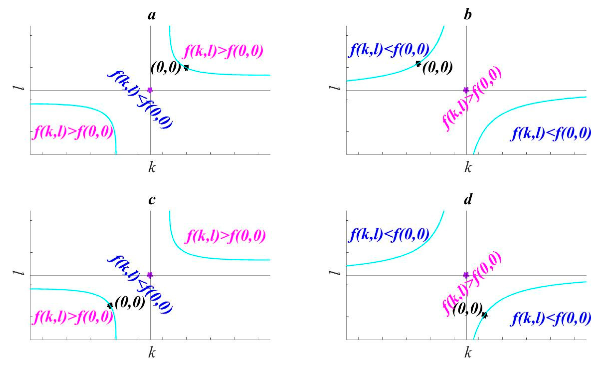
2.5. Function Properties and Graph

In this section, we discuss the properties and graphical representation of Equation (9). For simplicity, let

$$A=\langle X^{*},Y^{*}\rangle , B=\langle X^{*},T^{*}\rangle , C=\langle T^{*},Y^{*}\rangle , D=\langle T^{*},T^{*}\rangle , E=\langle X^{*},X^{*}\rangle , F=\langle Y^{*},Y^{*}\rangle ;$$

these are constants. Equation (9) can be written as

$$r_{X_{tr}{Y}_{tr}}=f(k,l)=\frac{A+Bl+Ck+Dkl}{\sqrt{E+2Bk+D{k}^2}\cdot \sqrt{F+2Cl+D{l}^2}}.$$

(13)

The first-order partial derivatives with respect to independent variables k and l are

$$f_k(k,l)=\frac{\partial f}{\partial k}=\frac{(C+Dl)(E+2Bk+D{k}^2)-(A+Bl+Ck+Dkl)(B+Dk)}{{(E+2Bk+D{k}^2)}^{\frac{3}{2}}\sqrt{F+2Cl+D{l}^2}},$$

(14)

$$f_l(k.,l)=\frac{\partial f}{\partial l}=\frac{(B+Dk)(F+2Cl+D{l}^2)-(A+Bl+Ck+Dkl)(C+Dl)}{\sqrt{E+2Bk+D{k}^2}{(F+2Cl+D{l}^2)}^{\frac{3}{2}}}.$$

(15)

Setting these two partial derivatives to zero, we can solve a simultaneous equation to obtain the stagnation point (k₀, l₀), i.e., the point at which the first-order partial derivatives are equal to zero:

$$\{\begin{array}{l}{k}_0=\frac{2A{B}^{2}C-A^{2}BD-B{C}^{2}E-B^{3}F+BDEF}{A^2{D}^2-2ABCD-D^{2}EF+C^{2}DE+B^{2}DF}\\ l_0=\frac{2AB{C}^2-A^{2}CD-B^{2}CF-C^{3}E+CDEF}{A^2{D}^2-2ABCD-D^{2}EF+C^{2}DE+B^{2}DF}\end{array}.$$

(16)

Taking the Taylor expansion of Equation (9) at the stagnation point $(k_0,l_0)$, we find that

$$\begin{array}{l}{r}_{X_{tr}{Y}_{tr}}=f(k,l)\\ \hspace{1em}\hspace{1em} =f(k_0,l_0)+\frac{1}{2}[\frac{{\partial }^{2}f}{\partial k^2}{|}_{(k_0,l_0)}{(k-k_0)}^2+2\frac{{\partial }^{2}f}{\partial k\partial l}{|}_{(k_0,l_0)}(k-k_0)(l-l_0)+\frac{{\partial }^{2}f}{\partial l^2}{|}_{(k_0,l_0)}{(l-l_0)}^2)]+o(\rho ),\end{array}$$

(17)

where $\frac{{\partial }^{2}f}{\partial k^2}{|}_{(k_0,l_0)}$ is the value of the second-order partial derivative of $f(k,l)$ with respect to k at the stagnation point $(k_0,l_0)$; $\frac{{\partial }^{2}f}{\partial l^2}{|}_{(k_0,l_0)}$ and $\frac{{\partial }^{2}f}{\partial k\partial l}{|}_{(k_0,l_0)}$ are similarly defined. The first term on the right-hand side is the value of f(k, l) at (k₀, l₀); this is independent of the trend coefficient, as will be explained later. The second term is the quadratic form of k and l, the graph of which is called a quadric surface, and this is obviously related to the trend coefficients. The third term is the Peano remainder, which is a high-order infinitesimal that can be neglected; $\rho =\sqrt{{(k-k_0)}^2+{(l-l_0)}^2}$, which means that as (k, l) approaches (k₀, l₀), $o(\rho )$ approaches zero faster. In the special case where the stagnation point (k₀, l₀) occurs at the origin, that is, (k₀, l₀) = (0, 0), Equation (17) takes the following form:

$$\begin{array}{l}{r}_{X_{tr}{Y}_{tr}}=f(k,l)\\ \hspace{1em}\hspace{1em} =f(0,0)+\frac{1}{2}[f_{xx}(0,0)k^2+2f_{kl}(0,0)kl+f_{ll}(0,0)l^2]+o(\sqrt{k^2+l^2}).\end{array}$$

(18)

This is the theoretical method for studying Equation (9), and requires the second-order partial derivatives to be obtained. However, the form of the first-order partial derivatives in Equations (14) and (15) is somewhat complex, making it difficult to find an analytical expression for the second-order partial derivatives. Thus, the remainder of this paper focuses on the graph of the function described in Equation (9).

To study the graph of Equation (9), as in Ref. [23], two time series X and Y with sample sizes of 68 are first generated at random. Their trend coefficients are −0.024 and 0.027, respectively, which are obviously very small. The time series X and Y are illustrated in Figure 1.

In statistical terms, there is no variation in the trends for time series X and Y, and we can consider the trend coefficients to be zero and their correlation coefficient to be −0.0035. In Ref. [23], a large number of simulations are used to superimpose the trend changes on time series X and Y in order to determine the correlation coefficient with respect to k and l (see Figure 1 in Ref. [23]). However, we can plot the graph of this function directly through the analytical expression in Equation (9). Figure 2a shows the isoline form of Equation (9), where $(k,l)\in [-1,1]\times [-1,1]$; graphs of Equations (11) and (12) in the interval [−1, 1] are presented in Figure 2b,c. Substituting X and Y into the stagnation point formula (Equation (16)), we find that the coordinates of the stagnation point are (0.024, −0.027), which happen to be the trend coefficients of X and Y with opposite signs; this coincidence has not been proven theoretically.

The equation of the two white hyperbolae in Figure 2a is $f(k,l)=f(0,0)\equiv -0.0035$, which is one contour line of Equation (9). The coordinate origin, marked by the white star, is located on the upper branch. The correlation coefficient of time series X and Y is −0.0035, which means that the superimposed trend coefficient is zero. The purple star denotes the stagnation point at (0.024, −0.027), where the function value is −0.0029 and the correlation between X and Y has effectively been detrended. Thus, the superimposed trend coefficient is the opposite of the trend coefficient. From Figure 2a, we can see that the graph of Equation (9) forms a saddle surface, so the stagnation point is a saddle point. Taking different time series X and Y and conducting numerical experiments, we find that all function graphs form a saddle surface, but the degree of deformation of the saddle varies for different time series. All of these function graphs have the same spatial structure, that is, the lower-left and upper-right corners are high-value areas where the function value is larger than at the saddle point, and the upper-left and lower-right corners are low-value areas where the function value is smaller than at the saddle point. The coordinate plane is divided into two parts by the white hyperbolae, namely, the part between the two branches and the area outside (above and below) the branches. When the superposition coefficients (k, l) lie between the two branches, the function value is greater than −0.0035, which indicates that when the superposed linear trend coefficients are in this range, the correlation coefficient is greater than this value. In contrast, when the superposition coefficients (k, l) are above the upper branch or below the lower branch of the hyperbolae, the function value is less than −0.0035, indicating that the correlation coefficient will be less than this value. Because the absolute value of the trend coefficient of time series X and Y is small, and the saddle point is very close to the coordinate origin, the white hyperbolae coincide with the coordinate axis. In addition, the correlation coefficient of X and Y is close to zero, so the above conclusion can be approximately described as follows: when k > 0 and l > 0 (or when k < 0 and l < 0), the correlation coefficient becomes larger and the positive correlation increases; when k > 0 and l < 0 (or when k < 0 and l > 0), the correlation coefficient is smaller and the negative correlation increases. This is the conclusion reached from Figure 1 in Ref. [23].

We now explore the symmetry of the graph of Equation (9). From Figure 2a, we can see that the graph is approximately axisymmetric with respect to the line l − l₀ = k − k₀ or l − l₀ = −(k − k₀), and is approximately centrosymmetric with respect to the saddle point at (k₀, l₀). Thus, the graph has good quasi-symmetry, but not strict symmetry. At the same time, we can see that although the graph is a saddle surface, it is slightly deformed compared with the standard saddle surface. In Figure 2b, when l = 0, the correlation coefficient increases monotonically with k; this monotonicity is caused by the distortion of the saddle surface. The same is true for Figure 2c, but these conclusions are not general. When taking different time series X and Y, the graph may first increase and then decrease, or vice versa.

In this experiment, the time series X and Y are randomly generated and their trend coefficients are −0.024 and 0.027, so we can imagine that there is no actual trend. More generally, let us consider the result when the trend coefficients of time series X and Y are large. It is almost impossible to generate sample data with a clear trend at random. In Ref. [23], no further research along this direction was reported. Thus, we select time series X and Y from meteorological data. Take China’s temperature and precipitation data from 1951–2019 as X and Y. These time series have 68 data points, trend coefficients of 0.36 and 0.34, respectively, and a correlation coefficient of 0.32, after standardization. The data are illustrated in Figure 3.

After standardization, X* and Y* are substituted into Equation (9), the graph of which is shown in Figure 4a. As the absolute value of the trend coefficient is limited to a maximum of 1.0, the range of the independent variable k in Figure 4 is [−1.36, 0.64] and the range of l is [−1.34, 0.66]. The rest of the illustration is exactly the same as in Figure 2a. By substituting X and Y into Equation (16), we find that the coordinates of the stagnation point are (−0.36, −0.34), which are the trend coefficients of X and Y with the opposite signs.

The graph of the correlation coefficient function in Figure 4a is also a deformed saddle surface. The white hyperbolae have the equation f(k, l) = f(0, 0) = 0.32. The coordinate origin, marked by the white star, is located on the upper branch; the saddle point is denoted by the purple star at (−0.36, −0.34), where the function value is 0.22. Similar to Figure 2a, the high-value areas of the saddle surface are in the lower-left and upper-right corners, and the low-value areas are in the upper-left and lower-right corners. However, the white hyperbolae are now in the lower-left and upper-right quadrants of the coordinate plane. Again, the coordinate plane can be divided into two parts, the area between the two hyperbolae and the area outside (above and below) the branches. When the superposition coefficients (k, l) lie between the two branches, the function value is less than f(0, 0) = 0.32, that is, the function value becomes smaller; in contrast, the function value will be larger than f(0, 0) = 0.32 when the superposition coefficients (k, l) are above the upper branch or below the lower branch. For example, the coordinates of point A are (−0.1, 0.6) and the correlation coefficient is 0.34 (>0.32); the coordinates of point B are (0.3, −0.13) and the correlation coefficient is 0.3 (<0.32). Comparing Figure 2a and Figure 4a, we can see that the saddle point is obviously further away from the origin in Figure 4a. This is because there is a significant trend in the selected time series and the correlation coefficient of X and Y is not close to zero. Thus, the approximate conclusion reached from Figure 2a cannot be applied here. We also know that, for different time series, the coordinate origin may be located to the upper-right, upper-left, lower-right, or lower-left of the saddle point. The graph of Equation (12) in the interval [−1.36, 0.64] is presented in Figure 4b, and the graph of Equation (11) in [−1.34, 0.66] is presented in Figure 4c. The differences between Figure 2b,c and Figure 4b,c are caused by the twisting deformation of the surface. There is no need to repeat the arguments, but for different time series X and Y, the function monotonicity may change, and this may be caused by the distortion of the saddle surface.

To summarize the above two experiments, the graph of Equation (9) is a deformed saddle surface, and the saddle point coordinates are the trend coefficients of time series X and Y with the opposite signs. The high-value areas are the lower-left and upper-right corners of the saddle, whereas the low-value areas are the upper-left and lower-right corners of the saddle. The isoline f(k, l) = f(0, 0) produces hyperbolae that divide the coordinate plane into two parts. For the different locations given by the trend coefficients (k, l), we can determine whether the correlation coefficient becomes larger or smaller after superposing the trend items, allowing us to quantitatively evaluate the influence of the trend item on the correlation coefficient.

In detail, when two time series are given, the correlation is determined by two factors, namely, the trend coefficient and the inherent correlation coefficient. We have discussed the influence of the trend coefficient on variations in the correlation coefficient. The terms containing both k and l in Equation (9) are the reason for these variations (The correlation coefficient is related to the size of the time series and the autocorrelation of each series, but this issue is not discussed in this article).

Let us briefly consider the Taylor expansion in Equation (17). The first term f(k₀, l₀) has been shown to be the correlation coefficient of time series X and Y after detrending, which has nothing to do with the trend and is an inherent attribute of time series X and Y. The second term is obviously related to the trend coefficients k and l. Therefore, the significance of Equation (17) is that it decomposes the correlation coefficient into the sum of the internal attributes and external environmentally induced term, that is, it separates the internal attributes from the external attributes inspired by the environmental field.

2.6. Operational Process

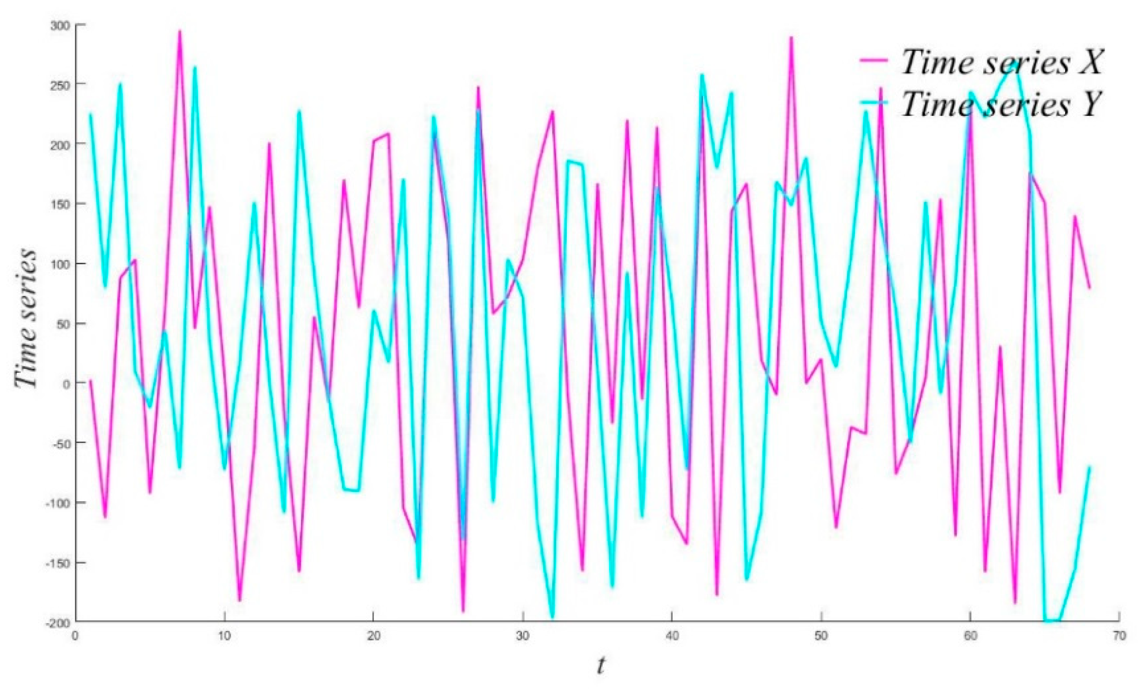
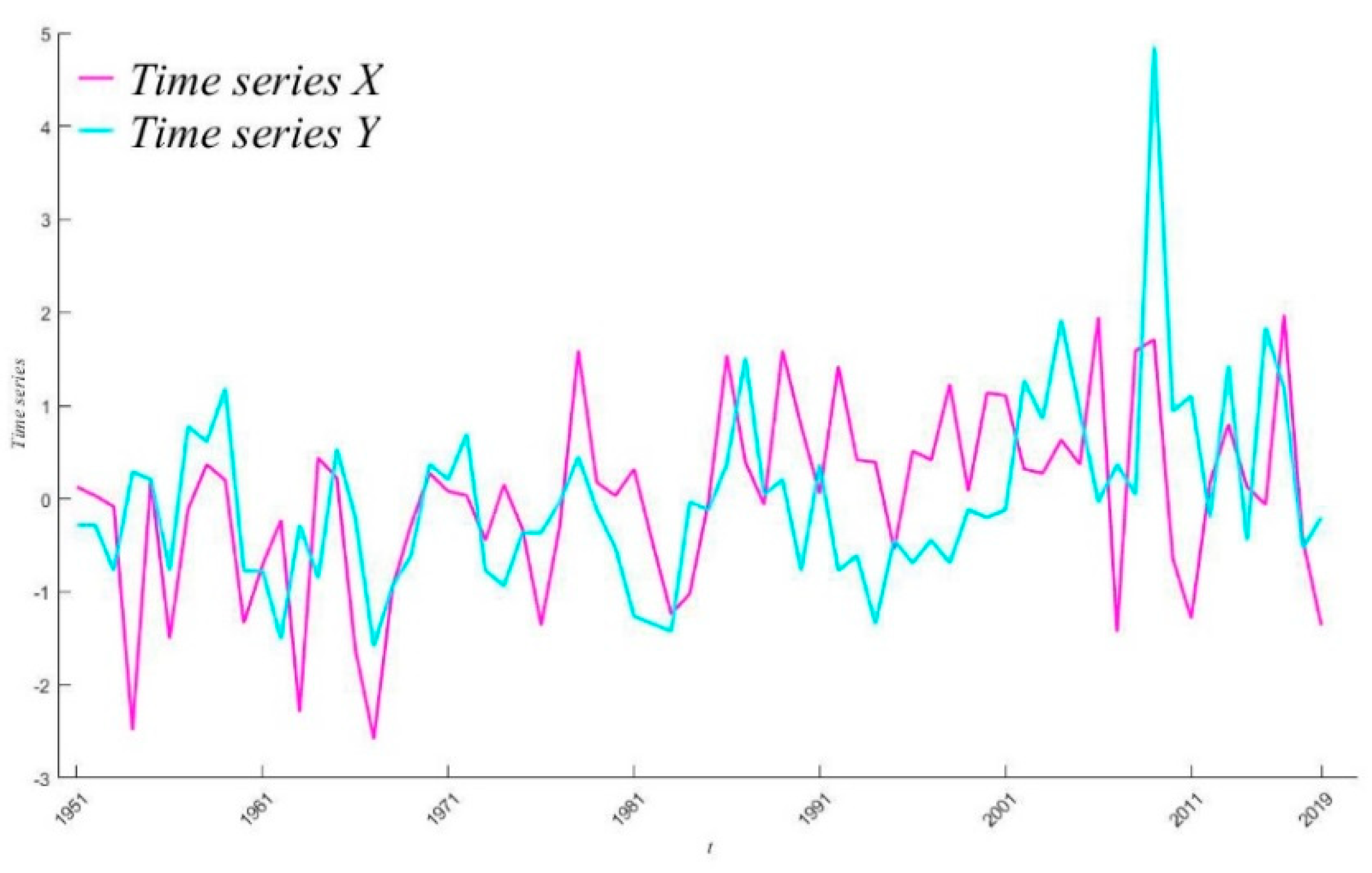
The process of checking the influence of the trend coefficients on the correlation coefficient is as described below.

Step 1: Time series X and Y are chosen arbitrarily.

Step 2: Calculate trend coefficients k and l of time series X and Y, respectively.

Step 3: Calculate correlation coefficient of X and Y after detrending; this only requires the calculation of f(−k, −l) in Equation (9), recorded as a = f(−k, −l).

Step 4: Calculate the correlation coefficient of X and Y; this only requires the calculation of f(0, 0) in Equation (10), recorded as b = f(0, 0).

Step 5: If k and l have the same sign, then a > b means that the correlation coefficient is increasing; if k and l have different signs, then a < b means that the correlation coefficient is decreasing.

Attention: As the coordinate axes are contours of the standard saddle surface, the graph f(k, l) is not a standard saddle surface, and the above conclusion is not applicable near the axes.

3. Two Examples

We obtained 100 datasets from 160 observation stations of the China Meteorological Administration, please see Supplementary Materials. The start time is the summer of 1951 and the end time is the spring of 2019, giving a data length of 68.

Test 1: Time series X contains spring data from the polar vortex area in the northern hemisphere (No. 50) with trend coefficient −0.72. Time series Y consists of spring precipitation data from the YuShu site (No. 144) with trend coefficient 0.41. Substituting X, Y, k = 0, and l = 0 into Equation (10), we found the correlation coefficient of X and Y to be −0.27. It was easy to find that the saddle point coordinates were (0.72, −0.41) and that the function value at the saddle point was 0.04 (correlation coefficient detrended). This indicates that when detrended, the correlation coefficient is 0.04, but the original correlation coefficient is −0.27. As k and l have different signs and −0.27 < 0.04, the trend terms increase the negative correlation (value becomes smaller).

Test 2: Time series X is taken as the winter data of the 850-hPa East Pacific Trade Wind (EPAC850, No. 85), which has a trend coefficient of −0.63. Time series Y is the winter precipitation data from the Duolun site (No. 26), where the trend coefficient is −0.38. The correlation coefficient between X and Y is 0.26, and the saddle point coordinates are (0.63, 0.38), where the function value is 0.03 (detrended). This indicates that when detrended, the correlation coefficient is 0.03, but the original correlation coefficient is 0.26. As k and l have the same sign and 0.26 > 0.03, the trend terms increase the positive correlation (value becomes larger).

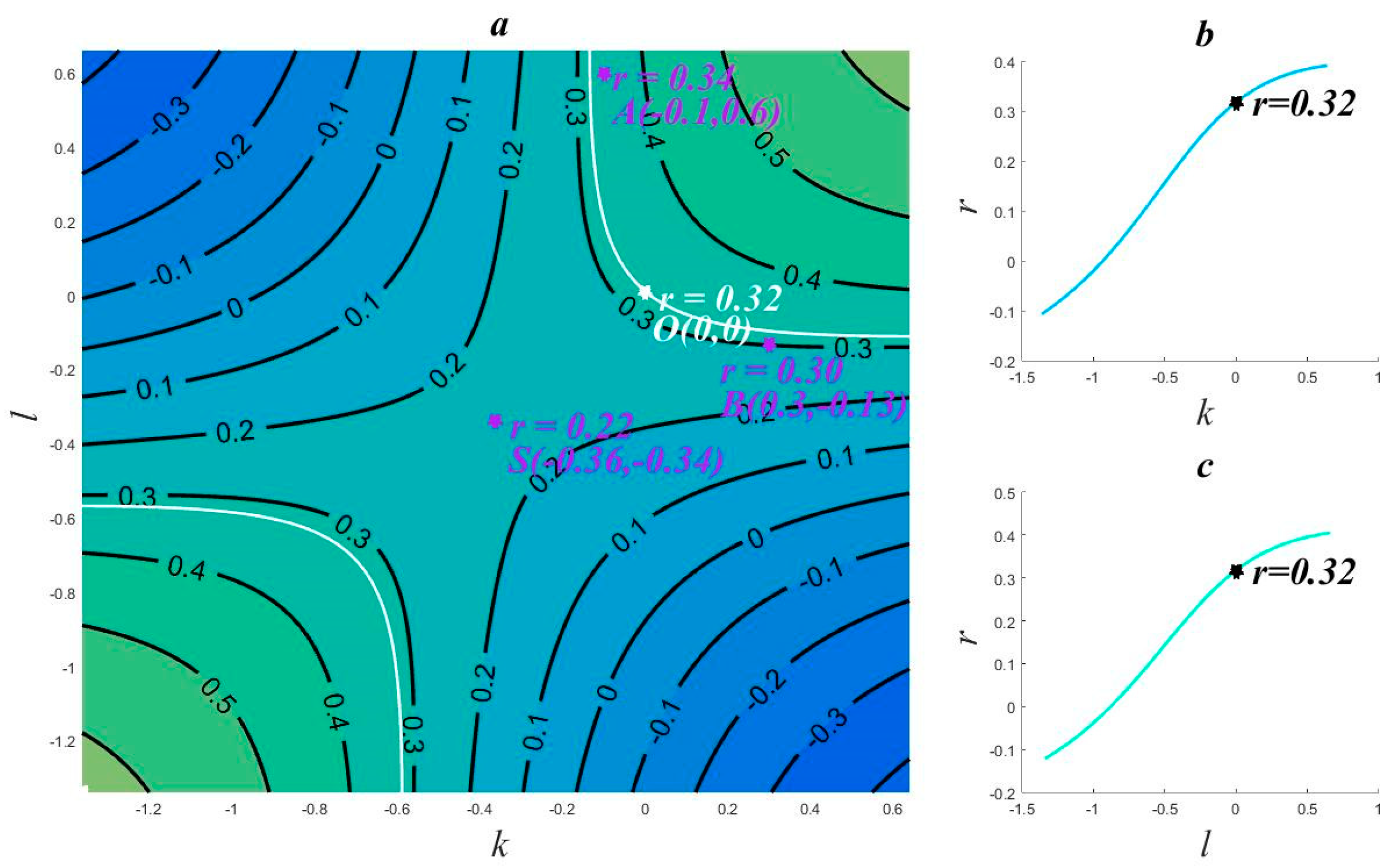
4. Spatial Distribution of Correlation Coefficient

In Figure 2a and Figure 4a, as well as in other numerical experiments, the positional relationship between the coordinate origin and the saddle point can be classified as one of four types: (i) the coordinate origin is to the upper-right of the saddle point; (ii) the coordinate origin is to the upper-left of the saddle point; (iii) the coordinate origin is to the lower-left of the saddle point; and (iv) the coordinate origin is to the lower-right of the saddle point. According to this classification, the distribution of the variation in the correlation coefficient with trend coefficients k and l is as shown in Figure 5. Figure 5a illustrates the first case, where the black star denotes the coordinate origin and purple star denotes the saddle point, and the light cyan lines are the isolines equal to f(0, 0). These lines divide the coordinate plane into two parts. In the region between the two cyan curves, we have f(k, l) < f(0, 0), and so the value of the correlation coefficient becomes smaller. In the regions above and below the cyan curve, f(k, l) > f(0, 0), and the value of the correlation coefficient becomes larger. The quasi-symmetry of the function graph means that Figure 5a is similar to Figure 5c, and Figure 5b is similar to Figure 5d.

5. Conclusions

This paper has discussed the influence of the trend coefficients of time series on the correlation coefficient. Our theoretical research produced the exact functional formula $r_{XtrYtr}=f(k,l)$ for the correlation coefficient in terms of the trend coefficients. Using a function expansion method, this formula was decomposed into the sum of the intrinsic correlation coefficient (detrended) and the term that varies with the trend. Numerical experiments were conducted for different time series X and Y, and in each case the graph of $r_{XtrYtr}=f(k,l)$ produced a saddle surface on which the saddle point coordinates were the trend coefficients of time series X and Y with opposite signs. Studying the function graph, we found that the isoline f(k, l) = f(0, 0) divides the coordinate plane into two parts where either f(k, l) > f(0, 0), in which case the correlation coefficient increases in magnitude, or f(k, l) < f(0, 0), in which case the correlation coefficient decreases. According to this, the spatial distribution of the correlation coefficient with respect to changes in the trend coefficients was derived. Two examples were presented to verify the practicality of the theory.

We can also see that the approach is based on a strict mathematical definition of the correlation coefficient. By deduction, the analytic expression of the correlation coefficient can be obtained with respect to the trend coefficients (k and l), so the proposed approach can be applied to general data. Although meteorological data were used in our case studies, the method is completely applicable to other types of data. Supplementary Material: Meteorological data.

In this paper, the time series displayed a linear trend, which is commonly observed in meteorological data. However, the trend of a time series may sometimes be nonlinear. In this case, Equations (4) and (5) become

$$X_{tr}=X^{*}+k(t)T^{*},$$

(19)

$$Y_{tr}=Y^{*}+l(t)T^{*},$$

(20)

where $k(t)$ and $l(t)$ are nonlinear functions that can be obtained using a curve fitting method. Similarly, Equation (9) becomes

$$r_{X_{tr}{Y}_{tr}}=F[k(t),l(t)]=\frac{\langle X^{*},Y^{*}\rangle +\langle X^{*},l(t)T^{*}\rangle +\langle k(t)T^{*},Y^{*}\rangle +\langle k(t)T^{*},l(t)T^{*}\rangle }{\sqrt{\langle X^{*},X^{*}\rangle +2\langle X^{*},k(t)T^{*}\rangle +\langle k(t)T^{*},k(t)T^{*}\rangle }\cdot \sqrt{\langle Y^{*},Y^{*}\rangle +2\langle Y^{*},l(t)T^{*}\rangle +\langle l(t)T^{*},l(t)T^{*}\rangle }},$$

(21)

where $r_{X_{tr}{Y}_{tr}}$ is a function of $k(t)$ and $l(t)$. This scheme works beautifully in theory, but the difficulty lies in identifying the universal trend functions $k(t)$ and $l(t)$. Our investigations show that the trend can be better represented by an exponential function for some time series, whereas a power function is better for others. Thus, determining the form of $k(t)$ and $l(t)$ will be the focus of future research.

References

1. IPCC. Climate Change 2013: The Physical Science Basis; Cambridge University Press: Cambridge, UK, 2013. [Google Scholar]
2. Kossin, J.P.; Emanuel, K.A.; Vecchi, G.A. The poleward migration of the location of tropical cyclone maximum intensity. Nature 2014, 509, 349–352. [Google Scholar] [CrossRef] [PubMed] [Green Version]
3. Zhao, Z.; Luo, Y.; Wang, S.; Huang, J.B. Scientific problems in global warming. J. Meteorol. Environ. 2015, 31, 1–5. [Google Scholar]
4. Jia, X.; Han, Q. Prediction and analysis of long-term trend of ground temperature by IAP AGCM model. Clim. Environ. Res. 2011, 16, 753–759. [Google Scholar]
5. Wang, Y.; Shi, N.; Gu, J.; Feng, G.; Zhang, L. Climate change in rainy days in China. Atmos. Sci. 2006, 30, 162–170. [Google Scholar]
6. Gocic, M.; Trajkovic, S. Analysis of changes in meteorological variables using Mann-Kendall and Sen’s slope estimator statistical tests in Serbia. Glob. Planet. Chang. 2013, 100, 172–182. [Google Scholar] [CrossRef]
7. Espinosa, L.A.; Portela, M.M.; Rui, R. Rainfall trends over a north atlantic small island in the period 1937/1938–2016/2017 and an early climate teleconnection. Theor. Appl. Climatol. 2021, 144, 1–23. [Google Scholar] [CrossRef]
8. Ayers, J.R.; Villarini, G.; Jones, C.; Schilling, K. Changes in monthly base flow across the U.S. Midwest. Hydrol. Processes 2019, 33, 748–758. [Google Scholar] [CrossRef]
9. Li, K.; Wang, A.; Zhao, T. Time delay analysis of broadband chaotic light generated by optoelectronic oscillator. J. Phys. 2013, 62, 144207. [Google Scholar]
10. Liang, S.X.; Qin, M.; Duan, J. Application of airborne cavity enhanced absorption spectroscopy system to the measurement of atmospheric No_2 with high spatial and temporal resolution. J. Phys. 2017, 66, 090704. [Google Scholar]
11. Shi, N.; Chen, J.; Tu, Q. Characteristics of climate change in China in the past 100 years. J. Meteorol. 1995, 53, 431–439. [Google Scholar]
12. Shi, N. Meteorological Statistical Forecast; Beijing Meteorological Press: Beijing, China, 2009. [Google Scholar]
13. Huang, J.P.; Yi, Y.H.; Wang, S.W.; Chou, J. An analogue-dynamical long-range numerical weather prediction system incorporating historical evolution. Q. J. R. Meteorol. Soc. 1993, 119, 547–565. [Google Scholar]
14. Huang, J. Significance test of meteorological element field. Meteorology 1989, 15, 3–7. [Google Scholar]
15. Wei, F. Modern Climate Statistical Diagnosis and Prediction Technology, 2nd ed.; Meteorological Press: Beijing, China, 2007. [Google Scholar]
16. He, G.; Su, Y.; Li, G.; Liu, B.H.; Meng, X.M. Correlation between in situ sound velocity and physical properties of marine sediments in the Central South Yellow Sea. J. Oceanogr. 2013, 35, 166–171. [Google Scholar]
17. Yu, C. Method and Application of Mathematical Geology; Metallurgical Industry Press: Beijing, China, 1980. [Google Scholar]
18. Li, T.; Ma, J. Application of correlation coefficient of earthquake fitting in earthquake prediction in Qinghai area. J. Earthq. Eng. 2008, 30, 184–188. [Google Scholar]
19. Wang, J.; Zhu, B.; Zhu, S. Remote sensing image stitching detection algorithm based on correlation coefficient. Mapp. Spat. Geogr. Inf. 2011, 34, 162–164. [Google Scholar]
20. Lu, D.; Zhao, W.Q.; Zeng, X.Y.; Wu, N.; Gao, G.T.; Zhang, Q.A.; Zhang, B.S.; Lei, Y.S. Relationship between stress relaxation characteristics and quality of kiwifruit ‘Hayward’. China Agric. Sci. 2019, 34, 201–206. [Google Scholar]
21. Wang, C.R.; Su, W.W.; Jiang, G.; Li, H.W.; Liang, Z.Q.; Yang, X.; Yuan, X.P.; Li, H.; Liao, F.C.; Ge, H.Z.; et al. Yangtze finless porpoise in Dongting Lake and its correlation with fish resources. Chin. Environ. Sci. 2019, 39, 4424–4434. [Google Scholar]
22. Fang, J. Statistical Methods of Biomedical Research; Higher Education Press: Beijing, China, 2007. [Google Scholar]
23. Shi, N.; Yi, Y.-M.; Gu, J.-Q.; Xia, D. On the correlation of nonlinear variables containing secular trend variations: Numerical experiments. Chin. Phys. 2006, 15, 2180–2184. [Google Scholar]
24. Kendall, M.A.; Stuart, A. The Advanced Theory of Statistics, 2nd ed.; Charles Griffin: Londres, UK, 1967. [Google Scholar]
25. Chandler, R.E.; Scott, M.E. Statistical Methods for Trend Detection and Analysis in the Environmental Analysis, 1st ed.; John Wiley & Sons: Chichester, UK, 2011. [Google Scholar]
26. Hamed, K.H. Exact distribution of the Mann–Kendall trend test statistic for persistent data. J. Hydrol. 2009, 365, 86–94. [Google Scholar] [CrossRef]
27. Peng, C.K. Havlin, S.; Stanley, H.E.; Goldberger, A.L. Quantification of scaling exponents and crossover phenomena in nonstationary heartbeat time series. Chaos 1995, 5, 82–87. [Google Scholar] [CrossRef] [PubMed]
Figure 1. Time series X and Y (trend coefficients of X and Y are −0.024 and 0.027, respectively).
Atmosphere 13 00066 g001
Figure 2. Graph of correlation coefficient function (trend coefficients of X and Y are −0.024 and 0.027, respectively). (a) r X t r Y t r = f ( k , l ) (left), (b) r X t r Y t r = f ( k ) (upper right), (c) r X t r Y t r = f ( l ) (lower right).
Atmosphere 13 00066 g002
Figure 3. Time series X and Y (trend coefficients of X and Y are 0.36 and 0.34, respectively).
Atmosphere 13 00066 g003
Figure 4. Graph of correlation coefficient function (trend coefficients of X and Y are 0.36 and 0.34, respectively). (a) r X t r Y t r = f ( k , l ) (left); (b) r X t r Y t r = f ( k ) (upper right); (c) r X t r Y t r = f ( l ) (lower right).
Atmosphere 13 00066 g004
Figure 5. Conceptual map of the spatial distribution of correlation coefficient with trend coefficient. Coordinate origin is to the (a) upper-right, (b) upper-left, (c) lower-left, and (d) lower-right of the saddle point.
Atmosphere 13 00066 g005
Publisher’s Note: MDPI stays neutral with regard to jurisdictional claims in published maps and institutional affiliations.