Abstract
This study used the FLEXPART-WRF trajectory model to perform forward and backward simulations of a cut-off low (COL) event over northeast Asia. The analysis reveals the detailed trajectories and sources of air masses within the COL. Their trajectories illustrate the multi-timescale deep intrusion processes in the upper troposphere and lower stratosphere (UTLS) caused by the COL. The processes of air intrusion from the lower stratosphere to the middle troposphere can be divided into three stages: a slow descent stage, a rapid intrusion stage and a relatively slow intrusion stage. A source analysis of targeted air masses at 300 hPa and 500 hPa shows that the ozone-rich air in the COL primarily originated from an extratropical cyclone over central Siberia and from the extratropical jet stream. The sources of air masses in different parts of the COL show some differences. These results can help explain the ozone distribution characteristics in the main body of a COL at 300 hPa and at 500 hPa that were revealed in a previous study.
1. Introduction
Stratosphere–troposphere exchange (STE) is an important dynamic process which takes place in the upper troposphere and lower stratosphere (UTLS). The STE primarily involves energy and mass exchange. Mass exchange refers to processes such as stratospheric air masses or chemical substances being transported downwards to the troposphere, as the water vapor and aerosols in the troposphere enter the stratosphere [1,2,3].
In the 1990s, the World Climate Research Program (WCRP) established the Stratospheric Processes and their Role in Climate (SPARC) core plan. Research carried out in recent decades has shown that the atmospheric composition budget and dynamics of the UTLS region play an important role in global radiation balance and climate change [4]. Therefore, the STE process in the UTLS region has become the focus of a great deal of research. The classical STE circulation model developed by Holton et al. [5] shows that the global STE is primarily controlled by the Brewer–Dobson circulation. The STACCATO plan [6] and START-05/08 experiments [7,8] launched in Europe and the Tibetan Plateau atmospheric composition program [9,10] conducted in China provided an improved depiction of the STE process related to synoptic and mesoscale systems in extratropical UTLS areas (Ex-UTLS), revealing an active stratosphere–troposphere air-mixing process. In the extratropical STE associated with the synoptic scale weather systems found in the Northern Hemisphere, the cut-off low (COL) is one of the most important systems. However, the specific mechanisms and details of the processes involved have not yet been elucidated. Studies of the source regions of air masses in the COL, along with their detailed movement trajectories and characteristics, still need to be further explored.
The COL is defined as a closed cold and low-pressure system, located in the middle to upper troposphere, which has grown out of a trough, having become completely detached from the basic westerly current in the jet stream, and subsequently lying equatorward of this westerly current [11]. COLs frequently occur in the regions of southern Europe, North America, and northeast China–Siberia [12]. Using aircraft observation, Bamber [13] discovered that an upper tropospheric air mass located within a 2 km thickness above the COL displays the properties of both the troposphere and the stratosphere. During the life cycle of COLs, the jet stream and tropopause fold can transport stratospheric air into the troposphere [14,15,16]. These findings were attributed to the mixing of air between the two atmospheric layers. The STE process caused by COLs is mainly driven by air moving along the isentropic surface [17], as well as by air moving across the isentropic surface caused by nonadiabatic processes such as wave breaking [18,19]; the latter is usually an irreversible deep mixing process. For the STE process caused by COLs in different regions, scientists have carried out observational data analysis and simulation research [20,21,22,23,24]. Škerlark et al. [25] used ERA-Interim ozone data to reveal the climatological process of stratospheric air intrusion caused by global COLs, while Akritidis et al. [26] used CAMS and MERRA-2 data to present the global climatology of tropopause folds.
Ozone sounding data [27,28], satellite data [29,30], and numerical simulations [31,32] were used to study the STE induced by COLs in northeast Asia. Using 89 validated ozone profiles in Changchun, China, Song et al. [28] revealed that COLs induced a 32% increase in the UTLS column ozone. Li et al. [30] applied the TRAJ3D trajectory model to analyze the air source of a COL event occurring over northeast Asia. Their results showed that air masses with a high ozone concentration in the center of the COL have two source regions: one is the polar vortex, and the other is the strong shear region on the cyclonic side of the extratropical jet axis. These studies have proven that COL is an important weather system that causes stratospheric ozone intrusion in northeast Asia, and which plays an important role in the distribution of atmospheric composition in the UTLS region.
Our current understanding of the detailed transport processes in the UTLS region induced by COLs over northeast Asia is still quite limited. Previous studies of the transport trajectory caused by COLs over northeast Asia have used the reanalysis data with every 6 h as a dynamic field to run the trajectory model [30]. In the present study, we use the Weather Research and Forecasting (WRF) model to simulate a typical case of COL over northeast Asia. The Lagrangian particle dispersion model FLEXPART driven by the WRF output, namely FLEXPART-WRF, was used to simulate the trajectories and the sources of air masses in this COL. Based on these results, the intrusions of the air mass on multiple time scales are further discussed. Compared with simulations using the reanalysis data to drive the trajectory model, the FLEXPART-WRF model uses the WRF model’s high spatio-temporal resolution outputs as its dynamic fields, thus better simulating the trajectories of air parcels.
The remainder of this paper was organized as follows: Section 2 briefly introduces the case, data source, and overview of this model. In Section 3, the simulations of the air parcel intrusion trajectories and the sources of targeted air masses in the COL were performed, and the simulation results were analyzed. Section 4 and Section 5 provide the discussion and main conclusions.
2. Case, Data, and Model
2.1. Case Overview
A typical case of COL was selected for model simulation, which occurred over northeast Asia on 19–23 June 2010. For this case, a series of studies were already carried out before. Its formation process and life cycle are consistent with the definition of COL found in the literature [12]. At 00:00 on 19 June (UTC, the same as below), a shallow trough over eastern Lake Baikal appeared in the middle and higher latitudes. With the deepening and southeastward extension of the trough, a cut-off cyclone formed at 06:00 on 20 June over northeast China. It intensified and reached its maximum intensity at 00:00 on 21 June. Then, it weakened at approximately 18:00 on 21 June and moved eastward out of northeast China. For details of the meteorological analysis, the synoptic configuration and dynamical tropopause related to this case, please refer to our past studies [31,33].
2.2. Data
Three datasets were used in this study. The final (FNL) operational global analysis data from the National Centers for Environmental Prediction and the National Center for Atmospheric Research (NCEP/NCAR) was taken as the initial field to drive the WRF model. This dataset contained 26 vertical layers, ranging from 1000 hPa to 10 hPa, with a horizontal resolution of 1° × 1°.
The ERA5 reanalysis data from the European Centre for Medium-Range Weather Forecasts (ECMWF) was used as the observational field to evaluate the simulation performance of the WRF model. This dataset contains 37 vertical layers, ranging from 1000 hPa to 1 hPa, with an hourly spatio-temporal resolution of 0.25° × 0.25°. The variables used in this study included the geopotential height, temperature, and horizontal wind.
The ozone distributions for the COL at 300 hPa and 500 hPa were provided by satellite observations from Level 2 ozone data, taken from atmospheric infrared sounder (AIRS) version 6 products. The AIRS satellite lies in a sun-synchronous polar orbit. It scans one revolution of the Earth in approximately 96 min, making a total of 15 revolutions per day. The horizontal and vertical resolutions of the AIRS data at the satellite’s nadir point are 13.5 km and 1 km, respectively, and the error in the ozone data of Level 2 below 0.5 hPa is 10–50% [34].
2.3. Model Introduction
The WRF is a next-generation high-resolution mesoscale meteorological model. It is used for various forecasting and analytical applications, ranging from the synoptic to global scale. WRF includes dozens of parameterizations for radiation, boundary layer processes, convection, microphysics, and land surface processes, which are designed to better improve the simulations and forecasts for synoptic systems.
The FLEXPART model, developed by the Norwegian Institute for Air Research, is a Lagrangian particle dispersion model [35]. It can simulate the long-range and mesoscale transport of tracers in the atmosphere by calculating the trajectories of particles (not necessarily representing real particles, but infinitesimally small air parcels) released from point, line, area or volume sources. The model can be extrapolated forwards in time to simulate the dispersion of tracers from their sources, or backwards in time to determine potential source contributions for given receptors.
The FLEXPART-WRF model is a combination of FLEXPART and WRF, where the FLEXPART model is driven by the output of the WRF model. An interface program for processing WRF outputs was added into the FLEXPART model, through which the processed WRF results can be directly adopted as initial data for the FLEXPART-WRF model. The initial meteorological field variables input to FLEXPART are pressure, geopotential, temperature, wind, specific humidity, TKE, and dew point. The FLEXPART model uses domain filling technology. Before the simulation is run, the atmosphere in three-dimensional space of the model on a regional scale, or even a global scale, is divided into a sufficient number of particles. These particles are then distributed within the model domain proportionally to air density. Each particle receives the same mass, with all particles taken together accounting for the total atmospheric mass. Subsequently, particles move within the atmosphere under the driving factors (i.e., wind, pressure, and temperature), after which the atmospheric transport process can be simulated. A detailed technical description of this model was given by Stohl et al. [35] and Brioude et al. [36], and the user guide is available at https://www.flexpart.eu/ (accessed on 20 December 2021).
This study started with using a WRF model to carry out a numerical simulation of a typical COL case occurring over northeast Asia. Based on the good performance of the WRF model in simulating this weather process, the results obtained from this model, such as geopotential height field, temperature field, and wind field with high spatio-temporal resolutions, were used to drive the FLEXPART model. In other words, the FLEXPART-WRF model (V3.1) was used to perform both the forward and backward trajectory simulations. The transport trajectories and sources of the air parcels in this case were then further studied, and the multi-timescale deep intrusions of the stratospheric air caused by the COL discussed in detail. It should be noted that, since the results of the WRF model are only used to drive the FLEXPART-WRF model, the evaluation of whether the WRF model is capable of reproducing this COL process is discussed in the Appendix A, while the main part of the paper primarily focuses on the analysis of the air movements inside the COL.
3. Results
3.1. Simulation of Air Parcel Intrusion Trajectories in the Cut-Off Low
The horizontal resolution of the WRF experiment was 27 km, while a substantially fine height resolution of ~300 m was used for the vertical resolution. The top of the model was set at 10 hPa, at a height of ~30 km. The WRF model outputs were used as the driving fields to provide meteorological field for the operation of the FLEXPART model. First of all, the FLEXPART-WRF model was used for the forward simulation of air parcels, aiming to reveal the air parcel trajectories and transportation characteristics within the COL in the UTLS region.
The simulation domain of the forward trajectory is 25–75° N, 80–150° E, with the vertical layer extending from 100 hPa to 700 hPa. A 4-day forward trajectory simulation was initiated at 17:00 on 18 June, ending at 18:00 on 22 June. At 17:00 on 18 June, a total of one million air parcels were placed into the simulated three-dimensional area based on air density distribution. They were distributed with a total mass of ~1.22 × 10¹² kg, and the value of the particle numbers and mass passed the significance test. The model output the air parcel information every hour, including longitude, latitude, altitude, potential vorticity (PV), and specific humidity.
STE can be divided into shallow exchange and deep exchange [37]. Deep intrusion is irreversible, and has a remarkable effect on the chemistry of the lower tropospheric [38]. In this study, we were aiming to investigate the deep intrusion of the stratospheric air parcels, which involves multi-timescale transport processes. In existing references [30,37,39], the criteria for deep stratospheric intrusion were defined as occurring when stratospheric air parcels cross the dynamical tropopause of 2 PVU (1 PVU = 10−6 K m2 kg−1 s−1) and penetrate levels below 700 hPa (or 600 hPa) within four days. Considering the characteristics of summer COLs over northeast Asia, for this study, deep stratospheric intrusion is defined as occurring when the air parcels cross the 2 PVU and 600 hPa surfaces within four days. Specifically, the criteria for deep stratospheric intrusion are as follows:
- (1)
- The PV of the air parcel at the initial position is greater than 2 PVU, and the specific humidity is smaller than 1 g kg−1 (this ensures that the air parcel came from above the 2-PVU isentropic surface and was located in the stratosphere at the initial time).
- (2)
- Air parcels must cross both the 2-PVU and the 600 hPa surfaces within 4 days (this ensures that the air parcel has experienced a deep intrusion).
- (3)
- Air parcels that cross both the 2-PVU and the 600 hPa surfaces, but not lying within the COL region, are eliminated from this study (this ensures that the deep intrusion of the air parcels was caused by the COL). This study region is defined as a circular area with a radius of 7° zonal distance, and the center point of the COL is defined as being at the center of this circle.
The targeted parcels in the forward trajectory were selected by means of the above criteria, and divided into three main different clusters based on their three-dimensional trajectories. Figure 1 shows the three-dimensional trajectories of parcels associated with deep intrusion. For further analyzing the features of deep intrusion, the time series of the average values of longitude, latitude, altitude (pressure), PV, and specific humidity along the trajectory of each cluster, are shown in Table 1.
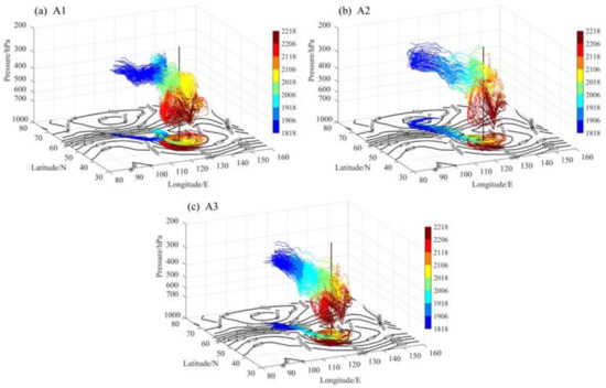
Figure 1.
Three-dimensional structure of trajectory clusters corresponding to A1 (a), A2 (b), and A3 (c). Color bars represent the 4-day forward trajectories of the air masses starting at 18:00 UTC on 18 June and ending at 18:00 UTC on 22 June, taken at 12 h intervals. The black contours represent the 500 hPa geopotential height, while the vertical black lines show the central position of the COL at 00:00 on 21 June. The projection of trajectories at the horizontal level are also shown.

Table 1.
Time series for the average values of longitude, latitude, pressure, PV, and specific humidity.
Combining Figure 1 and Table 1, it can be seen that the locations of the source regions for clusters A1 and A3 were very close to each other, both originating from the trough over the northern part of Lake Baikal (at approximately 55° N, 108° E), while air parcels in cluster A2 originated from the extratropical cyclone formed over the northern part of central Siberia (at approximately 70° N, 112° E). There are certain differences among the trajectories of these three clusters. Cluster A1 (Figure 1a), which originated near the northern part of Lake Baikal, moved southeastwards and then entered northeastern China from 18:00 on 18 June to 18:00 on 19 June. During the cut-off stage of the trough (from 18:00 on 19 June to 06:00 on 20 June), the air parcels cyclonically rotated one circle inside the trough before rapidly inclining downwards and intruding into the middle troposphere at approximately 500 hPa (from 06:00 on 20 June to 18:00 on 21 June). From 18:00 on 21 June to 18:00 on 22 June, the air parcels in cluster A1 in the middle troposphere rotated anticlockwise around the center of the COL and slowly moved downwards.
Visibly different from cluster A1, the air parcels in cluster A2, which originated in the extratropical cyclone over the northern of central Siberia (Figure 1b), slowly descended from the lower stratosphere from 18:00 on 18 June to 06:00 on 21 June. This process took one more day than in cluster A1 for the air parcels to reach 364 hPa (Table 1), after which they entered China via Mongolia. Subsequently, the air parcels rotated anticlockwise for one circle and then rapidly intruded downwards into the middle troposphere (~550 hPa) from 06:00 on 21 June to 18:00 on 22 June.
Cluster A3, which originated from the same source as cluster A1, was the deepest and fastest-moving cluster when intruding downwards (Figure 1c). The air parcels moved southeastward and passed through Mongolia to arrive in northeastern China. After that, they inclined downwards and rapidly intruded into the middle troposphere at approximately 520 hPa, from 18:00 on 18 June to 18:00 on 21 June. Subsequently, in the middle troposphere, the air parcels cyclonically revolved around the center of the COL and slowly moved downwards to reach approximately 600 hPa, from 18:00 on 21 June to 18:00 on June 22. This process is called “rotation” intrusion [30].
In general, from the air parcel trajectories revealed in Figure 1 and Table 1, it can be seen that in the UTLS region, as the trough develops, the stratospheric air masses slowly moved southwards from the bottom of the trough at higher latitudes, before rotating and slowly intruding downwards in the trough. When the trough was cut off (at 06:00 on 20 June), and as the COL developed, the air masses tilted downwards and quickly intruded into the middle troposphere at approximately 500 hPa. After that, the air masses rotated and were slowly transported downwards under the control of the anticlockwise circulation of the COL below 500 hPa. The simulation results of this trajectory support the results obtained by Li et al. [30] using the TRAJ3D model.
In addition, the average values of PV and specific humidity in Table 1 reveal that, along particle trajectories, the low specific humidity (high PV) in the stratosphere started to increase (decrease) as particles entered the troposphere. This is because of the mixing occurring between the dry air from the stratosphere and the moist air in the troposphere.
Figure 2 further shows the changes in average height of the air parcels in clusters A1–A3, as well as changes in the mean value of the average heights of the three clusters over time. It was found that the changes in average height over time are basically similar among the three clusters, but there are still some slight differences. For example, above 500 hPa, the height of cluster A3 more rapidly decreased, while cluster A2 was the slowest.
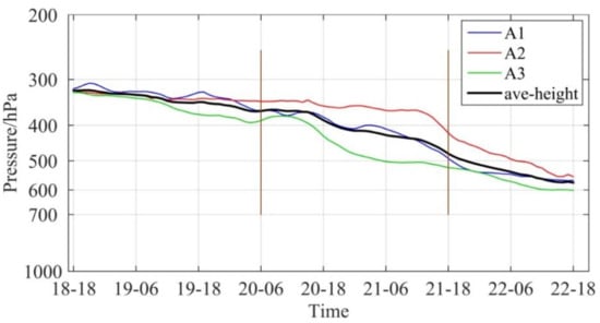
Figure 2.
Time series of the average pressure of air clusters A1–A3 (blue: A1; brown: A2; green: A3) and the mean value of the average pressure of the three clusters (black). The time in horizontal axis is day-hour.
According to the evolution of the COL described in Section 2.1, we divided its life cycle into three stages, referred to as the pre-formation stage, developmental and mature stage, and decay stage. By analyzing the mean value of the average heights of the three clusters over time (the black line), it was found that the movement trajectory of the air masses presented multi-timescale features. The first was a slowly descending stage, which was the development period of the upper trough (from 18:00 on 18 June to 06:00 on 20 June), corresponding to the pre-formation stage of the COL. The air masses were slowly transported downwards with the development of the upper trough, descending by approximately 921 m (from ~320 hPa to ~365 hPa) within 36 h. The second was a rapid intrusion stage. As the COL was cut off and rapidly developed (from 06:00 on 20 June to 18:00 on 21 June), this corresponded to the developmental and mature stage. The air masses rapidly intruded from the upper troposphere to the middle troposphere within 36 h, descending by approximately 2061.6 m (from ~365 hPa to ~490 hPa). Finally, there was a relatively slow intrusion stage (from 18:00 on 21 June to 18:00 on 22 June), which corresponded to the decay stage. The air masses dropped to approximately 500 hPa during the second stage. As affected by the anticlockwise circulation of the COL, the air masses slowly rotated and descended during this stage, extending downwards by approximately 1095.3 m (from ~490 hPa to ~573 hPa) within 24 h.
3.2. Simulation of the Sources of Targeted Air Parcels in the Main Region of the Cut-Off Low
Aiming to explore the sources of targeted air parcels in the main region of the COL and in order to further discuss the ozone transport processes in the UTLS region, the FLEXPART-WRF model was also applied to the backward trajectory simulation. The simulation area was 35–56° N, 110–150° E. A 3-day simulation was initiated at 19:00 on 21 June and ended at 18:00 on 18 June. A total of 10,000 air parcels were distributed in the simulation area at 300 hPa and 500 hPa according to the air density distribution at 19:00 on 21 June, with a total mass of ~1.22 × 10¹⁰ kg. Similar to the forward simulation, the values of both particle numbers and mass passed the significance test, and the model output the air parcel information every hour. These included the longitude, latitude, altitude, potential vorticity, and specific humidity.
It should be noted that, from the previous analysis, the 500 hPa is the key level and is located in the middle troposphere based on the COL structure. Meanwhile, the 300 hPa is approximately the level that the air concentrations are intermediate between typical tropospheric and stratospheric values. The targeted parcels were therefore selected at these two levels. Figure 3 displays the distributions of ozone at 300 hPa and 500 hPa from the AIRS satellite data at 18:00 on 21 June, superimposed by the geopotential height and PV from the ERA-Interim reanalysis data. At 300 hPa and 500 hPa, the main body of the COL corresponded to large-value areas of both ozone and PV. Therefore, according to the horizontal structure of the COL at 18:00 on 21 June, we selected the targeted parcels lying in the center, east, west, and south sides of the COL, which are, respectively, marked in blue, orange, red, and green (Figure 4), in order to analyze the source of the ozone-rich air masses and further discuss the multi-timescale transportation processes in the UTLS region.

Figure 3.
Ozone distributions (shaded, unit: ppmv) at 300 hPa (a) and 500 hPa (b) pressure surfaces at 18:00 on 21 June taken from the AIRS satellite data. The panels are superimposed by the geopotential height (gray dashed line, unit: gpm) and potential vorticity (black contour, unit: PVU) taken from the ERA-Interim reanalysis data.
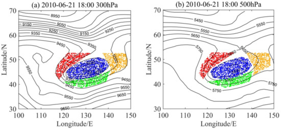
Figure 4.
Schematic diagram of the partition of target air parcels lying in the center (blue), east (orange), west (red), and south (green) side of the COL at 300 hPa (a) and 500 hPa (b).
The initial positions of the four parts of the targeted parcels in the main body of the COL at 300 hPa, along with their 3-day backward trajectories, are illustrated in Figure 5. Figure 6 provides the changes in the height of targeted parcels in each part. By jointly analyzing these two figures, the sources and transport characteristics of air parcels in each part of the COL are revealed.
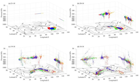
Figure 5.
The initial positions of the four parts of the targeted parcels in the main body of the COL at 300 hPa (a). Projection of the targeted parcels on the longitude–latitude, longitude–height, and latitude–height planes at 18:00 on 20 June (b), at 18:00 on 19 June (c) and at 18:00 on 18 June (d). The geopotential height (black contours, unit: gpm) are additionally plotted on each longitude–latitude plane. Colored dots indicate different clusters. The superimposed pink solid line in (d) represents the extratropical jet stream axis.
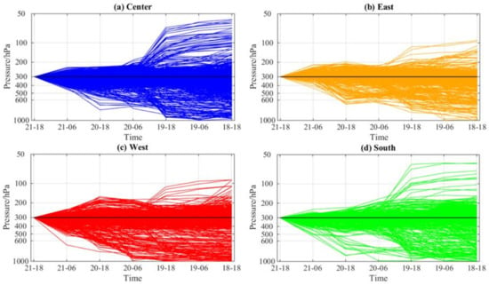
Figure 6.
The 3-day backward trajectory of the height of air parcels at the center (a), east (b), west (c), and south (d) sides of the COL at 300 hPa.
Air parcels in the central part of the COL (the blue cluster), those with the highest ozone concentration of all clusters, mainly originated from two sources—one was the extratropical cyclone over central Siberia, and the other was the cyclonic side of the extratropical jet stream (near 55° N, west of 80° E) (Figure 5d). The air parcels simultaneously represent both ascending and descending motion. They could quickly move downwards, from a level of 55 hPa to approximately 200 hPa within 36 h (from 18:00 on 18 June to 06:00 on 20 June), and then slowly descend to 300 hPa (Figure 6a).
On the east and west sides of the COL (the orange and red clusters), the ozone concentration was lower. Most of the air parcels came from the trough located at approximately 30–40° N (Figure 5d). The few descending air parcels in these two targeted regions originated from the extratropical cyclone and the extratropical jet stream, and then slowly descended from the lower stratosphere to 300 hPa (Figure 6b,c).
The air parcels on the south side of the COL (the green cluster) primarily came from the anticyclonic side of the extratropical jet stream (Figure 5d). The trajectory of the air parcels in this part was similar to that in the central part of the COL, where a small amount of air parcels could rapidly move from a level of 55 hPa down to approximately 200 hPa (Figure 6d).
Figure 7 and Figure 8 are the same as Figure 5 and Figure 6, respectively, but for 500 hPa. From Figure 7 and Figure 8, it can be seen that the air parcels in the central part (blue) of the COL mainly came from the extratropical cyclone over central Siberia and from the trough on the south of the cyclone. Most of the air parcels on the east side (orange) of the COL came from the trough located at approximately 30–40° N. The air parcels on the west side (red) of the COL mainly originated from the extratropical cyclone over central Siberia. The air parcels on the south side (green) of the COL mainly came from the anticyclonic side of the extratropical jet stream (Figure 7d). There was both ascending and descending motion observed for air parcels in the four targeted regions. The descending air parcels mainly intruded from approximately 300 hPa down to 500 hPa (Figure 8).
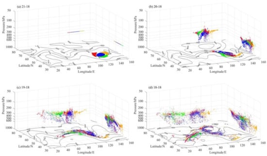
Figure 7.
The initial positions of the four parts of the targeted parcels in the main body of the COL at 500 hPa (a). Projection of the targeted parcels on the longitude–latitude, longitude–height, and latitude–height planes at 18:00 on 20 June (b), at 18:00 on 19 June (c) and at 18:00 on 18 June (d). The geopotential height (black contours, unit: gpm) are additionally plotted on each longitude–latitude plane. Colored dots indicate different clusters. The superimposed pink solid line in (d) represents the extratropical jet stream axis.
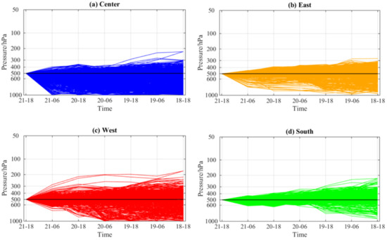
Figure 8.
The 3-day backward trajectory of the height of air parcels at the center (a), east (b), west (c), and south (d) sides of the COL at 500 hPa.
As Figure 6 and Figure 8 do not adequately illustrate the numbers of descending and ascending particles, Figure 9 further presents the proportion of descending and ascending particles for each part at 300 hPa and 500 hPa, respectively. If a particle was located above 300 hPa at 18:00 on 18 June, and continuously descended to 300 hPa over time, in this case, it belongs to the descending particles category. Similarly, the number of ascending particles can also be obtained, and hence, the total number of particles attained.
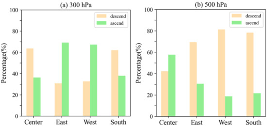
Figure 9.
Percentages of descending and ascending air parcels for each part at 300 hPa (a) and 500 hPa (b).
It can be seen from Figure 9a that the number of descending air parcels coming from above 300 hPa accounted for 63.7% of the total. This correspondingly produced a high ozone concentration area in the central part of the COL (Figure 3a). The proportion of ascending particles from below 300 hPa in the east and west parts were 69.2% and 67.3%, respectively. This indicated that it was mostly ozone-poor air from lower altitudes, undergoing an upward motion, caused the ozone concentration in the east and west parts of the COL to be much lower.
The target particles at 500 hPa mostly came from above 500 hPa, with the downward motion ending at 500 hPa. In the center, east, west, and south sides of the COL, the proportions of descending air parcels to the total were 42.3%, 69.4%, 81.3%, and 78.4%, respectively (Figure 9b). These descending air parcels illustrated that ozone-rich air masses probably intrude into the middle troposphere, or possibly even lower. It should be noted that, although the ozone concentration in the central part of the COL is at its highest value at 500 hPa, the number of descending particles is at its lowest, while the number of descending particles located at the periphery of the COL (east, west, and south parts) are much greater. We considered that these were probably affected by the anti-clockwise horizontal wind at the periphery of the COL between 300 hPa and 500 hPa, since the peripheral air parcels of the COL primarily showed a rotating descending motion (as the results from the forward trajectory revealed, as outlined in Section 3.1). Therefore, the number of descending particles is greater than those inside the central part of the COL. However, the ozone-rich air masses came from the stratosphere, while the descending air parcels in the central area came from a higher altitude; thus, even if the proportion of descending air parcels in the central part is lower, a high ozone concentration can still be maintained.
4. Discussion
According to the forward and backward simulations carried out for this study, as the COL developed, the air parcels in the lower stratosphere rapidly intruded downwards as the tropopause descended, finally reaching the upper troposphere. Subsequently, the air parcels rotated anticlockwise around the center of the COL and slowly descended to the middle troposphere. This “fast intrusion” in the upper troposphere and “slow intrusion” in the middle troposphere reflected multi-timescale intrusions within the transport processes of the air masses. Therefore, this can to some extent explain the ozone distribution characteristics in the main body of the COL at 300 hPa in the upper troposphere, and at 500 hPa in the middle troposphere, which were revealed in our previous study [40]. In that study, a large amount of reanalysis data and satellite data were used to statistically analyze the spatio-temporal distributions of ozone in the UTLS region using a total of 186 COL events. The results showed that the area with a higher ozone concentration in the upper troposphere (300 hPa) was distributed around the center of COLs, which coincided with the distribution of high PV. In the middle troposphere (at 500 hPa), there were two regions with enhanced levels of ozone concentration, with the highest being located to the east of COLs, and the second highest in the center of COLs. This spatial distribution of ozone in the upper troposphere was mainly affected by the descending, or folding, of the tropopause. The ozone was subjected to a “rotary” transport process in the middle troposphere, primarily influenced by the anticlockwise circulation of the COLs and the surrounding horizontal wind distribution. From the analysis of the intrusion trajectories and time scales of the transport processes carried out in this study, the explanation given by Chen et al. [40] was further confirmed.
This study revealed the multi-timescale transport processes of the deep intrusion in the UTLS associated with a COL, and provided a foundation for the detailed description of the STE process caused by textratropical weather systems. However, it does have its limitations, as it only simulates and analyzes one single COL case; trajectories and sources of air masses in COLs with different intensities and of different types may be different. Therefore, further studies are needed in this area.
5. Conclusions
Cut-off lows are synoptic-scale systems that play an important role in STE within the Ex-UTLS. This study first used the WRF model to simulate the typical case of a COL over northeast Asia, and then applied the output of the WRF model to drive a FLEXPART-WRF model to carry out both forward and backward simulations. The aim was to reveal the detailed trajectories and sources of the air masses inside the COL, and to discuss the intrusions on different time scales.
The trajectory of the air masses presented multi-timescale features, and the process in the UTLS region could thus be divided into three stages. The first stage was the slow descending stage, which was also the development period of the upper trough. The air masses slowly transported downward as the upper trough developed, descending by approximately 921 m within 36 h. The second was the rapid intrusion stage. The air masses rapidly intruded from the upper troposphere into the middle troposphere within 36 h, descending by approximately 2061.6 m. The third stage was a relatively slow intrusion stage. Since they were affected by the anticlockwise circulation of the COL, the air masses slowly rotated and descended from the middle troposphere during this stage, extending downwards by approximately 1095.3 m within 24 h.
In the upper troposphere (300 hPa), the air masses in the central part of the COL primarily originated from an extratropical cyclone over central Siberia and from the cyclonic side of the extratropical jet stream. On the east and west sides of the COL, most of the air masses came from the trough located at approximately 30–40° N. The air masses on the south side of the COL mainly came from the anticyclonic side of the extratropical jet stream. In the middle troposphere (500 hPa), the air masses in the central part of the COL primarily came from the extratropical cyclone over central Siberia and the trough located to the south of this cyclone. Most of the air masses on the east side of the COL came from the trough located at approximately 30–40° N. The air masses on the west side of the COL mainly originated from the extratropical cyclone over central Siberia. The air masses on the south side of the COL mainly came from the anticyclonic side of the extratropical jet stream.
The forward and backward simulations revealed that, with the development of the COL, the air masses in the lower stratosphere rapidly intruded downwards as the tropopause descended, before reaching the upper troposphere. Subsequently, the air masses rotated anticlockwise around the center of the COL and slowly descended to the middle troposphere. The “fast intrusion” in the upper troposphere and the “slow intrusion” in the middle troposphere reflect the features of multi-timescale intrusion during the transportation processes of air masses.
Author Contributions
Conceptualization, D.C.; investigation and methodology, D.C. and T.Z.; formal analysis, software and visualization, T.Z. and S.G.; writing—original draft preparation, T.Z. and D.C.; writing—review and editing, D.C. and D.G.; supervision, D.G. All authors discussed the results and commented on the paper and figures. All authors have read and agreed to the published version of the manuscript.
Funding
This work was funded by the National Natural Science Foundation of China (42175069, 91837311, 41305038).
Institutional Review Board Statement
Not applicable.
Informed Consent Statement
Not applicable.
Data Availability Statement
The dataset of FNL analysis data is available at https://rda.ucar.edu/datasets/ds083.2/ (accessed on 20 December 2021). The reanalysis data were obtained from ECMWF are available at https://apps.ecmwf.int/datasets/ (accessed on 20 December 2021) and https://cds.climate.copernicus.eu/ (accessed on 20 December 2021). AIRS satellite data are also freely available at https://disc.gsfc.nasa.gov/datasets (accessed on 20 December 2021). The information of FLEXPART-WRF is available at https://www.flexpart.eu/ (accessed on 20 December 2021).
Acknowledgments
We acknowledge the NCAR, ECMWF and Climate Change Service for providing the analysis and reanalysis data. Furthermore, we would like to thank the team of the AIRS instrument for their continued effort in maintaining and continuously improving the AIRS dataset. We also would like to thank the team of the FLEXPART model to develop and share it.
Conflicts of Interest
The authors declare no conflict of interest.
Appendix A. Numerical Experiment and Validation of the COL Case
Appendix A.1. Numerical Experiment
The Advanced Research Weather Research and Forecasting model (WRF-ARW) of version 3.8 was used to simulate the evolution of a COL occurring on 19–23 June 2010. A 4.5-day time integration was carried out from 12:00 UTC on 18 June to 00:00 UTC on 23 June. A single domain was assigned to the defined region, as shown in Figure A1. This time period and region covered the entire COL area and life cycle. The horizontal resolution was 27 km, and a substantially fine height resolution of ~300 m was used for the vertical. The top of the model was set to 10 hPa, at a height of ~30 km. Conventional physical parameterization schemes were used, which have also previously been applied to our published works [31,33]; these include the Lin microphysics scheme, the Kain–Fritsch cumulus parameterization scheme, the YSU planetary boundary layer scheme, the RRTM long-wave radiation scheme, and the Dudhia short-wave radiation scheme. The model variables were saved at 30 min time intervals.

Figure A1.
Domain of the model, and tracks of the simulated (blue dots ‘●’) and the real (red triangles ‘▲’) cut-off low. The horizontal axis is longitude, and the vertical axis is latitude.
Figure A1.
Domain of the model, and tracks of the simulated (blue dots ‘●’) and the real (red triangles ‘▲’) cut-off low. The horizontal axis is longitude, and the vertical axis is latitude.

Appendix A.2. Validation of the Simulated Characteristic of the COL Case
By using the ERA5 analysis and modeling data, the grid point with the lowest value at 500 hPa geopotential height was selected as the center of the COL. Its movements are plotted in Figure A1, which is confined to the period from 06:00 UTC on 20 June to 06:00 UTC on 22 June, taken at 6 h time intervals. Figure A1 shows that the simulated track is in good agreement with the ERA5 analysis over the two days.
Taking 06:00 UTC on 19 June and 06:00 UTC on 21 June as an example, detailed comparisons of the simulated geopotential height and temperature at 500 hPa and 200 hPa isobaric maps with the ERA5 analysis, are shown in Figure A2 and Figure A3, respectively. Combining Figure A2 and Figure A3, it can be seen that the model results can well simulate the process of the continuous deepening of the trough to the South, and the formation of the COL. The simulated geopotential height and temperature distributions agreed well with the ERA5 data. Additionally, there was good agreement in terms of the location and intensity of the COL, both in the cold core at 500 hPa (Figure A2d), as well as in the warm core at 200 hPa (Figure A3d).


Figure A2.
The 500 hPa geopotential height (solid lines, unit: gpm) and temperature (dash–dot lines, unit: °C) from the ERA5 data (a,c) and the simulation (b,d), at 06:00 UTC on 19 June, and at 06:00 UTC on 21 June, respectively.
Figure A2.
The 500 hPa geopotential height (solid lines, unit: gpm) and temperature (dash–dot lines, unit: °C) from the ERA5 data (a,c) and the simulation (b,d), at 06:00 UTC on 19 June, and at 06:00 UTC on 21 June, respectively.


Figure A3.
The 200 hPa geopotential height (solid lines, unit: gpm) and temperature (dash–dot lines, unit: °C) from the ERA5 data (a,c) and the simulation (b,d), at 06:00 UTC on 19 June, and at 06:00 UTC on 21 June, respectively.
Figure A3.
The 200 hPa geopotential height (solid lines, unit: gpm) and temperature (dash–dot lines, unit: °C) from the ERA5 data (a,c) and the simulation (b,d), at 06:00 UTC on 19 June, and at 06:00 UTC on 21 June, respectively.

A comparison of the simulated horizontal wind on 300 hPa isobaric maps and the meridional cross-section of the horizontal wind at 130° E (taken at 06:00 UTC on 21 June) with the ERA5 analysis data are shown in Figure A4. The results show that the jet stream near 62° N and the jet stream surrounding the COL were well reproduced (Figure A4a,b). Moreover, in the meridional cross-section, there was good agreement between the ERA5 analysis data (Figure A4c) and the simulation results (Figure A4d). For example, the distribution of the wind field and the height of the jet stream core near 300 hPa were very similar using both methods.

Figure A4.
The 300 hPa horizontal wind (unit: m/s) from the ERA5 data (a), the simulation (b), and the meridional cross-section of horizontal wind at 130° E from the ERA5 data (c) and from the simulation (d) at 06:00 UTC on 21 June.
Figure A4.
The 300 hPa horizontal wind (unit: m/s) from the ERA5 data (a), the simulation (b), and the meridional cross-section of horizontal wind at 130° E from the ERA5 data (c) and from the simulation (d) at 06:00 UTC on 21 June.

In conclusion, the comparison showed that the model was able to accurately reproduce the temperature–pressure features and the horizontal wind structure during the life cycle of the COL. These results also indicated that the simulation data of the WRF model can be used to construct the initial fields required for driving the FLEXPART model, and that the FLEXPART-WRF model is thus suitable for carrying out further research on the simulation of air trajectories inside a COL.
References
- Kremser, S.; Thomason, L.W.; Hobe, M.V.; Hermann, M.; Deshler, T.; Timmreck, C.; Toohey, M.; Stenke, A.; Schwarz, J.P.; Weigel, R.; et al. Stratospheric aerosol—Observations, processes, and impact on climate. Rev. Geophys. 2016, 54, 278–335. [Google Scholar] [CrossRef]
- Yu, P.; Toon, O.B.; Bardeen, C.G. Black carbon lofts wildfire smoke high into the stratosphere to form a persistent plume. Science 2019, 365, 587–590. [Google Scholar] [CrossRef] [PubMed]
- Wang, Y.P.; Wang, H.Y.; Wang, W.K. A stratospheric intrusion-influenced ozone pollution episode associated with an intense horizontal-trough event. Atmosphere 2020, 11, 164. [Google Scholar] [CrossRef]
- Gettelman, A.; Hoor, P.; Pan, L.L.; Randel, W.J.; Hegglin, M.I.; Birner, T. The extratropical upper troposphere and lower stratosphere. Rev. Geophys. 2011, 49, RG3003. [Google Scholar] [CrossRef]
- Holton, J.R.; Haynes, P.H.; McIntyre, M.E.; Douglass, A.R.; Rood, R.B.; Pfister, L. Stratosphere-troposphere exchange. Rev. Geophys. 1995, 33, 403–439. [Google Scholar] [CrossRef]
- Stohl, A.; Bonasoni, P.; Cristofanelli, P.; Collins, W.; Feichter, J.; Frank, A.; Forster, C.; Gerasopoulos, E.; Gäggeler, H.; James, P.; et al. Stratosphere-troposphere exchange: A review, and what we have learned from STACCATO. J. Geophys. Res. Atmos. 2003, 108, D12. [Google Scholar] [CrossRef]
- Pan, L.L.; Bowman, K.P.; Shapiro, M.; Randel, W.J.; Gao, R.S.; Canpos, T.; Davis, C.; Schauffler, S.; Ridley, B.A.; Wei, J.C.; et al. Chemical behavior of the tropopause observed during the Stratosphere-Troposphere Analyses of Regional Transport experiment. J. Geophys. Res. 2007, 112. [Google Scholar] [CrossRef]
- Pan, L.L.; Bowman, K.P.; Atlas, E.L.; Wofsy, S.C.; Zhang, F.; Bresch, J.F.; Ridley, B.A.; Pittman, J.V.; Homeyer, C.R.; Romashkin, P.; et al. The stratosphere-troposphere analyses of regional transport 2008 experiment. Bull. Am. Meteorol. Soc. 2010, 91, 327–342. [Google Scholar] [CrossRef]
- Guo, D.; Su, Y.C.; Shi, C.H.; Xu, J.J.; Powell, A.M. Double core of ozone valley over the Tibetan Plateau and its possible mechanisms. J. Atmos. Sol.-Terr. Phys. 2015, 130–131, 127–131. [Google Scholar] [CrossRef]
- Guo, D.; Su, Y.C.; Zhou, X.J.; Xu, J.J.; Shi, C.H.; Liu, Y.; Li, W.L.; Li, Z.K. Evaluation of the trend uncertainty in summer ozone valley over the Tibetan Plateau in three reanalysis datasets. J. Meteorol. Res. 2017, 31, 431–437. [Google Scholar] [CrossRef]
- Gimeno, L.; Trigo, R.M.; Ribera, P.; García, J.A. Editorial: Special issue on cut-off-low systems (COL). Meteorol. Atmos. Phys. 2007, 96, 1–2. [Google Scholar] [CrossRef]
- Nieto, R.; Gimeno, L.; Torre, L.D.L.; Ribera, P.; Gallego, D.; García, J.A.; Nunez, M.; Redano, A.; Lorente, J. Climatological features of cutoff low systems in the Northern Hemisphere. J. Clim. 2005, 18, 3085–3103. [Google Scholar] [CrossRef]
- Bamber, D.J.; Healey, P.G.W.; Jones, B.M.R.; Penkett, S.A.; Tuck, A.F.; Vaughan, G. Vertical profiles of tropospheric gases: Chemical consequences of stratospheric intrusions. Atmos. Environ. 1984, 18, 1759–1766. [Google Scholar] [CrossRef]
- Price, J.D.; Vaughan, G. Statistical studies of cut-off-low systems. Ann. Geophys. 1992, 10, 96–102. [Google Scholar]
- Ancellet, G.; Beekmann, M.; Papayannis, A. Impact of a cutoff low development on downward transport of ozone in the troposphere. J. Geophys. Res. 1994, 99, 3451–3468. [Google Scholar] [CrossRef]
- Langford, A.O.; Masters, C.D.; Proffitt, M.H.; Hise, E.Y.; Tuck, A.F. Ozone measurements in a tropopause fold associated with a cut-off low system. Geophys. Res. Lett. 1996, 23, 2501–2504. [Google Scholar] [CrossRef]
- Wirth, V. Diabatic heating in an axisymmetric cut-off cyclone and related stratosphere-troposphere exchange. Q. J. R. Meteor. Soc. 1995, 121, 127–147. [Google Scholar] [CrossRef]
- Price, J.D.; Vaughan, G. The potential for stratosphere-troposphere exchange in cut-off-low systems. Q. J. R. Meteorol. Soc. 1993, 119, 343–365. [Google Scholar] [CrossRef]
- Homeyer, C.R.; Bowman, K.P.; Pan, L.L.; Atlas, E.L.; Gao, R.S.; Campos, T.L. Dynamical and chemical characteristics of tropospheric intrusions observed during START08. J. Geophys. Res. 2011, 116, D06111. [Google Scholar] [CrossRef]
- Hoor, P.; Wernli, H.; Hegglin, M.I. Transport timescales and tracer properties in the extratropical UTLS. Atmos. Chem. Phys. 2010, 10, 7929–7944. [Google Scholar] [CrossRef]
- Yates, E.L.; Iraci, L.T.; Roby, M.C.; Pierce, R.B.; Johnson, M.S.; Reddy, P.J.; Tadić, J.M.; Loewenstein, M.; Gore, W. Airborne observations and modeling of springtime stratosphere-to-troposphere transport over California. Atmos. Chem. Phys. 2013, 13, 12481–12494. [Google Scholar] [CrossRef]
- Dempsey, F. Observations of stratospheric O-3 intrusions in air quality monitoring data in Ontario, Canada. Atmos. Environ. 2014, 98, 111–122. [Google Scholar] [CrossRef]
- Schwartz, M.J.; Manney, G.L.; Hegglin, M.I.; Livesey, N.J.; Santee, M.L.; Daffer, W.H. Climatology and variability of trace gases in extratropical double-tropopause regions from MLS, HIRDLS, and ACE-FTS measurements. J. Geophys. Res. 2015, 120, 843–867. [Google Scholar] [CrossRef]
- Akritidis, D.; Katragkou, E.; Zanis, P.; Pytharoulis, I.; Melas, D.; Flemming, J.; Inness, A.; Clark, H.; Plu, M.; Eskes, H. A deep stratosphere-to-troposphere ozone transport event over Europe simulated in CAMS global and regional forecast systems: Analysis and evaluation. Atmos. Chem. Phys. 2018, 18, 15515–15534. [Google Scholar] [CrossRef]
- Škerlak, B.; Sprenger, M.; Pfahl, S.; Tyrlis, E.; Wernli, H. Tropopause folds in ERA-Interim: Global climatology and relation to extreme weather events. J. Geophys. Res. 2015, 120, 4860–4877. [Google Scholar] [CrossRef]
- Akritidis, D.; Pozzer, A.; Flemming, J.; Inness, A.; Zanis, P. A global climatology of tropopause folds in CAMS and MERRA-2 reanalyses. J. Geophys. Res. Atmos. 2021, 126, e2020JD034115. [Google Scholar] [CrossRef]
- Bian, J.; Gettelman, A.; Chen, H.; Pan, L.L. Validation of satellite ozone profile retrievals using Beijing ozonesonde data. J. Geophys. Res. Atmos. 2007, 112. [Google Scholar] [CrossRef]
- Song, Y.; Lü, D.; Li, Q.; Bian, J.; Wu, X.; Li, D. The impact of cut-off lows on ozone in the upper troposphere and lower stratosphere over Changchun from ozonesonde observations. Adv. Atmos. Sci. 2016, 33, 135–150. [Google Scholar] [CrossRef]
- Shi, C.; Li, H.; Zheng, B.; Guo, D.; Liu, R. Stratosphere-troposphere exchange corresponding to a deep convection in warm sector and abnormal subtropical front induced by a cutoff low over East Asia. Chin. J. Geophys. 2014, 57, 1–10. [Google Scholar]
- Li, D.; Bian, J.C.; Fan, Q.J. A deep stratospheric intrusion associated with an intense cut-off low event over East Asia. Sci. China Earth Sci. 2015, 58, 116–128. [Google Scholar] [CrossRef]
- Chen, D.; Lü, D.R.; Chen, Z.Y. Simulation of the stratosphere-troposphere exchange process in a typical cold vortex over Northeast China. Sci. China Earth Sci. 2014, 57, 1452–1463. [Google Scholar] [CrossRef]
- Wu, X.; Lü, D.R. Calculation of stratosphere-troposphere exchange in East Asia cut-off lows: Cases from the Lagrangian perspective. Atmos. Ocean. Sci. Lett. 2016, 9, 31–37. [Google Scholar] [CrossRef][Green Version]
- Chen, D.; Chen, Z.Y.; Lü, D.R. Simulation of the generation of stratospheric gravity waves in upper-tropospheric jet stream accompanied with a cold vortex over Northeast China. Chin. J. Geophys. 2014, 57, 10–20. [Google Scholar]
- Parkinson, C.L. Aqua: An earth-observing satellite mission to examine water and other climate variables. IEEE Trans. Geosci. Remote Sens. 2003, 41, 173–183. [Google Scholar] [CrossRef]
- Stohl, A.; Forster, C.; Frank, A.; Seibert, P.; Wotawa, G. Technical note: The Lagrangian particle dispersion model FLEXPART version 6.2. Atmos. Chem. Phys. 2005, 5, 2461–2474. [Google Scholar] [CrossRef]
- Brioude, J.; Arnold, D.; Stohl, A.; Cassiani, M.; Morton, D.; Seibert, P.; Angevine, W.; Evan, S.; Dingwell, A.; Fast, J.D.; et al. The Lagrangian particle dispersion model FLEXPART-WRF version 3.1. Geosci. Model. Dev. 2013, 6, 1889–1904. [Google Scholar] [CrossRef]
- Wernli, H.; Bourqui, M. A Lagrangian “1-year climatology” of (deep) cross-tropopause exchange in the extratropical Northern Hemisphere. J. Geophys. Res. 2002, 107, ACL13. [Google Scholar] [CrossRef]
- Stevenson, D.S.; Dentener, F.J.; Schultz, M.G.; Ellingsen, K.; van Noije, T.P.C.; Wild, O.; Zeng, G.; Amann, M.; Atherton, C.S.; Bell, N.; et al. Multimodel ensemble simulations of present-day and near-future tropospheric ozone. J. Geophys. Res. 2006, 111, D08301. [Google Scholar] [CrossRef]
- Sprenger, M.; Wernli, H. A northern hemispheric climatology of cross-tropopause exchange for the ERA15 time period (1979–1993). J. Geophys. Res. Atmos. 2003, 108, D12. [Google Scholar] [CrossRef]
- Chen, D.; Zhou, T.J.; Ma, L.Y.; Shi, C.H.; Guo, D.; Chen, L. Statistical Analysis of the Spatiotemporal Distribution of Ozone Induced by Cut-Off Lows in the Upper Troposphere and Lower Stratosphere over Northeast Asia. Atmosphere 2019, 10, 696. [Google Scholar] [CrossRef]


Publisher’s Note: MDPI stays neutral with regard to jurisdictional claims in published maps and institutional affiliations. |
© 2021 by the authors. Licensee MDPI, Basel, Switzerland. This article is an open access article distributed under the terms and conditions of the Creative Commons Attribution (CC BY) license (https://creativecommons.org/licenses/by/4.0/).