Abstract
A majority of the annual precipitation in many mountains falls as snow, and obtaining accurate estimates of the amount of water stored within the snowpack is important for water supply forecasting. Mountain topography can produce complex patterns of snow distribution, accumulation, and ablation, yet the interaction of topography and meteorological patterns tends to generate similar inter-annual snow depth distribution patterns. Here, we question whether snow depth patterns at or near peak accumulation are repeatable for a 10-year time frame and whether years with limited snow depth measurement can still be used to accurately represent snow depth and mean snow depth. We used snow depth measurements from the West Glacier Lake watershed, Wyoming, USA, to investigate the distribution of snow depth. West Glacier Lake is a small (0.61 km2) windswept (mean of 8 m/s) watershed that ranges between 3277 m and 3493 m. Three interpolation methods were compared: (1) a binary regression tree, (2) multiple linear regression, and (3) generalized additive models. Generalized additive models using topographic parameters with measured snow depth presented the best estimates of the snow depth distribution and the basin mean amounts. The snow depth patterns near peak accumulation were found to be consistent inter-annually with an average annual correlation coefficient (r2) of 0.83, and scalable based on a winter season accumulation index (r2 = 0.75) based on the correlation between mean snow depth measurements to Brooklyn Lake snow telemetry (SNOTEL) snow depth data.
1. Introduction
In snow dominated areas, it is important to understand the quantity and distribution of snow for purposes of streamflow forecasting [1]. In mountainous terrain, one of the most apparent characteristics of the snowpack is its spatial heterogeneity [2,3,4,5,6,7,8]. Mountain topography can produce complex patterns of snow distribution, accumulation, and ablation [9]. The snowfall deposition and snowmelt patterns are a result of temporally consistent interactions between the localized meteorology and terrain [10]. Different studies have identified topography, solar radiation, wind, slope, aspect, and vegetation as important drivers that control snow depth and snow water equivalent (SWE) variability [5,10,11,12,13,14,15,16,17,18,19]. The resultant distribution of snow often has a similar pattern from year to year [16,20] based on topography, canopy, if present, and wind characteristics, i.e., speed and direction [14,15]. These distribution patterns and the associated topography (and canopy) dictate further distribution and ablation processes [19] that dictate peak streamflows out of the basin [21], baseflow characteristics [22], and groundwater recharge [23].
Grayson et al. [20] identified three distinct ways to identify patterns: (1) “lots of points” (LOP), where there is a sufficiently dense array of point measurements to be interpolated to a pattern; (2) “binary data”, such as the presence or absence of snow cover; and (3) “surrogate data”, used to create correlations between the snow and easily established patterns such as topography and vegetation. Snow depth distribution studies utilize at least one or more of these three sampling methods. For example, topographic parameters are used to explain the spatial heterogeneity of snow depth through statistical approaches, including linear regression models [24,25], multiple linear regression models [18,19], binary regression trees [5,13,14,26], general additive models [27,28], and geostatistical models [5,15,17,29].
Results suggest that winter season indices can be applied to consistent snow patterns [15,16,20]. The character of a winter season can be defined by features including temperature averages and extremes [30], snowfall totals [30,31], snow depth [30,31], and the winter duration [32]. A snowfall index [31], a snow drift factor [33], a winter season severity index [30], and a climatological grid index [16] have all been used to evaluate and improve distributed snow models [33,34,35]. A winter season index allows quantities such as averages, percentiles, and extremes to be calculated to establish a baseline year across individual years [30]. Such an index would compare snowpack characteristics, such as depth, in a particular year to the long-term average.
Snow accumulation and distribution patterns are often consistent over time [3,10,15,16,20,36,37,38]. This leads to the question: are spatial patterns sufficiently consistent across years with abundant measurements so that we can confidently use sparse measurements in other years to extrapolate the snowpack patterns? Here, we evaluate whether snow depth distribution patterns are consistent over a 10-year period within a sub-alpine basin, West Glacier Lake, in Wyoming, U.S.A., and whether spatial patterns are sufficiently consistent across years with abundant measurements so that we may confidently use sparse measurements in other years to extrapolate the snowpack patterns and estimate basin mean snow depth. The specific questions for this study are as follows: (1) Do snow depth measurements reveal a consistent snow depth distribution over time? (2) What snow depth interpolation model provides the best representation of snow depth distribution? (3) What are the dominant topographic parameters that control snow distribution, and do they vary over time? (4) Can a winter season index be used to quantify basin snow depth?
2. Study Site
The study site is the West Glacier Lake watershed (WGLW) in the Snowy Range Mountains, Wyoming (41°22′30″ N latitude and 106°15′30″ W longitude) (Figure 1a). WGLW is part of the US Forest Service’s Glacier Lakes Ecosystem Experiments Site (GLEES) developed to conduct research on the effects of atmospheric deposition on alpine and subalpine ecosystems [39]. Approximately 5.75 km2 in size, GLEES consists of three small watersheds beneath a northeast–southwest ridge. WGLW is 0.61 km2 in size and ranges in elevation from 3277 m at the lake outlet to 3493 m at the top. The landscape contains Engelmann spruce (Picea engelmannii) and subalpine fir (Abies lasiocarpa) forests with some limber pine (Pinus flexilis) in the lower portions and krummholz stands of the same species at the higher elevations (~40%); bare rock outcrops (~48%); open water (~7%); and a permanent snow field (~5%) [29,39]. The mean annual temperature is −1 °C at the outlet and −2.5 °C at the top of the basin [40]. Mean annual precipitation is 1200 mm, with approximately 75 to 85% falling as snow, which typically remains from late October to early June [36,40]. Large inter-annual and spatial variability exists among measured precipitation quantities [29,41], as seen at the five precipitation monitoring stations within 4 km of GLEES: National Atmospheric Deposition Program (NADP) WY00 and WY95, Clean Air Status and Trends Network (CASTNET), GLEES Tower, and Brooklyn Snowpack Telemetry (SNOTEL). This region is dominated by strong westerly winds that range between 0 and 26 m/s with an average of 8 m/s [40]. Topographic and consistent climatic conditions within the region create an optimal environment to evaluate whether snow distributions repeat over time [35].
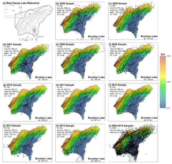
Figure 1.
(a) Topographic map of West Glacier Lake watershed. Snow depth sample locations and summary statistics for sample year (b–k) 2005 to 2014, and (l) all year locations (n = 3382).
3. Data and Methods
3.1. Survey Data
Snow depth data were collected by manual snow surveys across the WGLW from 2005 through 2014, during or close to peak snow accumulation each year (generally late April to early May) on an approximate 50 m measurement grid using an aluminum snow depth probe with 0.01 m graduations (purchased from https://snowmetrics.com/, last accessed 3 December 2021) [41]. Snowpacks in the WGLW usually exhibit a large spatial variability, and topographic parameters apply a strong, but consistent control on their distribution. At each snow depth measurement location, either three or five snow depth measurements were recorded to the nearest 0.01 m, and the locations were recorded with a global positioning system (GPS) with an approximate horizontal accuracy of +/− 5 m. Multiple snow depth measurements were taken at a specific location to limit the effect of local anomalies related to microtopography, rocks, woody material, or other limitations of reaching the ground surface [42] and to account for grid size scale uncertainty [5,7,43]. The mean snow depth was obtained by averaging all the measurements at a specific location.
The advantage of analyzing a multiyear data set is that it allows for the evaluation of topographic controls and to identify whether snowpack depths are consistent across years. From measurement years 2005 through 2009, between 400 and 500+ measurement locations were collected; the measured snow depth data contained similar sampling spatial distributions across the entire watershed and measurements had similar summary statistics (mean, standard deviation, and coefficient of variation) for those five years (Figure 1; Table 1). This is compared to the between 100 and 300 measurements collected near peak snow accumulation between 2010 and 2014, with inconsistent snow depth sample locations across the basin and a focus on the lower elevations and flatter terrain (Figure 1; Table 1). Therefore, the snow depth measurement years were split into two groups for modeling and evaluation: (1) measurement years 2005 through 2009 were used to determine whether a consistent snow depth distribution could be identified and if this snow depth distribution could be quantified and (2) the remaining measurement years, 2010 through 2014, were used to evaluate reduced measurement location years.

Table 1.
Summary of snow depth sample measurements for WGL snow surveys, concurrent Brooklyn Lake SNOTEL snow depth measurements, and simulated snow depth statistics. The difference and percent difference are calculated from the sample basin mean depth to the simulated basin mean depth.
3.2. Topographic Parameters
Seven topographic parameters (called parameters since they do not change over time) of elevation, slope, aspect, northness, solar radiation, water ponding, and maximum upwind slope (see Appendix A) were considered as independent variables in snow depth models to improve the interpolated estimates [5,12,13,44,45,46]. Vegetation was not used as a predictor due to the limited vegetation within WGLW. A 5 m digital elevation model (DEM) was generated by the U.S. Forest Service (USFS) based on aerial photographs and infrared imagery [47], and these data were used to derive all topographic parameters. A description of the parameter derivation is provided in Appendix A.
The topographic parameter elevation was considered since precipitation generally increases with elevation due to orographic lifting [2,11,48,49,50]. Even in low relief basins, small changes in elevation can alter snow distribution processes through wind scour and deposition. Slope is an important terrain feature affecting the snow depth distribution [51]. In topographically similar terrain, snow depth can be exposed to high wind shear forces: a slope that is oriented toward the mean wind direction tends to have a decrease in snow depth whereas a downwind-facing slope tends to have an increase in snow depth [48]. Aspect has been attributed to the snowmelt effect [11]. The exposure of the slope aspect to the sun can affect solar radiation inputs, which in turn controls snowpack temperature and stability [49,52]. Solar radiation influences snowmelt. Northness is commonly considered as a substitute for solar effects [5]. A solar radiation index was calculated for the basin for the 15th of each month from December to April, as per previous research [5,12,13]. The average monthly value for the five dates was used as an index of direct solar radiation during the accumulation season [53].
Water ponding depth is a parameter used to delineate drainage paths and depressions [44]. In windswept landscapes, such as GLEES [36], it can be an indicator of a topographic low points where there is significant snow accumulation [44,54]. Water ponding represents the depth (m) of surface depression on the surface in regard to the surroundings in elevation [44]. To capture this process, a ponding depth [44] parameter was estimated and used in the modeling of snow depth distribution.
Strong winds interact with local topography and are critical to the creation of heterogeneous snow depth distribution, often cited as one of the dominant influences on snow accumulation and distribution [3,5,14,19,35,55]. Accounting for wind interactions is a crucial process to aid in the understanding of snow distribution and snow variability. To capture this process, a wind shelter index [56] was used to aid in the modeling of snow depth distribution.
3.3. Interpolation Methods
In this study, we compared three commonly used interpolation methods (binary regression tree, multiple linear regression, and generalized additive models) that are applied in snow depth distribution research. The binary regression tree (BRT) method and multiple linear regression (MLR) models were selected for ease of calculation, interpretation of results, and due to previous success in snow distribution studies [5,7,13,42,45,57]. Generalized additive model (GAM) methods were selected for the ease of calculation, the ability to capture non-linear interactions, and due to previous success in snow distribution studies [27,28,46,58]. More details on these methods are provided in Appendix B. Models with the lowest deviance and highest coefficient of determination (r2) were selected.
The calibration measurement years 2005 through 2009 were used to assess the three interpolation methods (Table 1). To assess the accuracy of the interpolation methods, cross-validation was used to compare the estimated and the observed values. The predicted snow depth values were used to calculate error estimates such as mean absolute error (MAE), root mean squared error (RMSE), and Willmott’s index of agreement (D) statistics [59].
To evaluate the calibration years, we ran the optimal model type using data from four of the five focus years (2005 to 2009) and omitted one year at a time. Fit statistics were computed from each four-year modeled snow depth and the snow depth observed in the omitted year. Residuals were computed between the modeled snow depth values and those observed in the omitted year. The correlation coefficient was computed between the residuals and each of the seven topographic parameters to identify any spatial bias.
3.4. Standardized Snow Depth Distribution
Our study focused on the repeatability of snow depth distributions using the model interpolated snow depth distributions and observed snow depth measurement locations across WGLW from different years. We examined the modeled snow depth distributions to the observed snow depth data to correlate snow depth patterns from different years. Modeled snow distributions for each year were standardized by the basin mean snow depth based on snow depth measurements. Standardized snow depth values (SDV) were calculated based on the methods of Sturm and Wagner [16]:
where di is the modeled snow depth at grid cell I and μd is the survey snow depth measurement location’s mean snow depth for year y. From the 2005 through 2009 SDV patterns, we developed a climatological snow distribution pattern (CSDP) by calculating the arithmetic mean of five survey patterns [16].
3.5. Climatological Snow Distribution Pattern Uncertainty
To quantify the uncertainty in snow depth distribution of the estimated SDV grids that were used to estimate the CSDP, we conducted a Monte Carlo analysis that used repeated random sampling of input variables to calculate a distribution of output variables. Monte Carlo methods utilize computational algorithms to model the probability of different outcomes in a process that cannot easily be predicted due to the intervention of random variables and/or uncertainty [60]. We repeated the random sampling process 2000 times, resulting in a distribution of CSDP values based on the mean and standard deviation of the scaled snow depth grids.
3.6. SNOTEL Data and Winter Season Index
The Natural Resources Conservation Service (NRCS) operates a snow pillow sensor at the Brooklyn Lake SNOTEL site (3121 m). Table 1 shows the snow depth measured at the SNOTEL site obtained from the USDA NRCS website (https://www.wcc.nrcs.usda.gov, last accessed 27 October 2021) during the snow depth measurement dates compared to the WGLW mean measurement depth. The WGLW measurements occurred near or at the peak SWE date. Since the Brooklyn Lake SNOTEL site is within 2 km of WGLW, these data were used to scale the SDV distribution within a WGLW.
A winter season index was estimated based on the ordinary least squares (OLS) correlation between mean snow depth measurements by year to Brooklyn Lake SNOTEL snow depth data by year following methods discussed in Erickson et al. [15] and Mayes Boustead et al. [30]. The OLS correlation was investigated for the five calibration years and for all 10 sample years. The winter snow depth season index was applied to the CSDP to provide a direct scaling of snow depth distribution for WGLW. The scaled snow depth was calculated by
where SDi is the snow depth at grid point i, CSDPi is the climatological snow distribution pattern snow depth at grid point i, and WSDindex,y is the winter snow depth season index for year y.
4. Results
4.1. Snow Survey Data
The snow depth distribution was modeled using 10 years with a total of 3382 depth measurements (each representing the mean of three or five measurements per location) (Figure 1), ranging from 118 measurements in 2011 to 538 measurements in 2005 (Table 1). The 10 years encompassed normal snow years, as well as record dry (2012) and wet (2011) snow years. Most other datasets have fewer snow depth measurements and/or fewer years of data [29]. The average snow depth ranged from 173 to 285 cm with an annual coefficient of variation (CV) ranging from 0.37 to 0.62 (Table 1); these values are within the range of 0.33 to 0.63 reported by Elder et al. [3]. A summary of each of the 10 years is presented in Table 1. The spatial extent of measurements varied inter-annually due to weather conditions, the number and experience of field personnel, and safety concerns (Figure 1), with the snow depth measurements ranging from 0 to 505 cm (Table 1).
4.2. Selection of Model
Three interpolation models were used to estimate the dependent variable of snow depth. We used the 2006 snow depth data set to evaluate the performance of the three interpolation methods. The 2006 data set was selected based on a balance between sample distribution and the number of sample points; although 2006 had the least amount of sample points (by twelve), it had a larger standard deviation and coefficient of variation, which provide a more robust data set to test interpolation methods. The best predictor was the GAM model with an MAE, RMSE, and D of 68 cm, 86 cm, and 0.715, respectively, with a basin mean snow depth of 197 cm (Figure 2a). The MLR model provided a decent representation of the snow depth distribution and the influence of wind redistribution, but had overall poor snow depth estimates: the MAE, RMSE, and D were 86 cm, 103 cm, and 0.396, respectively, with a basin mean snow depth of 190 cm (Figure 2b). The pruned ten node BRT model has a similar basin mean snow depth (196 cm), but provided the poorest snow depth distribution estimate, similar to that of López-Moreno and Nogués-Bravo [27]. The topographic and wind redistribution parameters were not well represented around the lake (Figure 2c), as illustrated by the error statistics for this method (MAE of 86 cm, RMSE of 109 cm, and Willmott’s D of 0.552). The MLR and GAM methods provided better estimates; from our results (Figure 2) and the literature [27,28,46,58], we used GAM methodology with topographic parameters to estimate the distribution of snow depth across the study domain for the subsequent analysis.
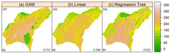
Figure 2.
The distribution of snow depth computed using three statistical interpolation techniques: (a) GAM, (b) linear regression, and (c) binary regression tree for 2006. The mean snow depth (cm) is presented in the upper left corner, and error statistics are presented in the lower left (mean absolute error or MAE) and lower right corner (Willmott’s D).
All seven topographic parameters were identified as significant predictors of the WGL distribution of snow depth for at least two of the five calibration years (2005–2009, Table 2). Slope was statistically significant for all calibration years, with elevation being significant for all years except 2009 and aspect being significant for three years (Table 2). Ponding was significant (p < 0.05) in one year and moderately significant (p < 0.1) for three years (Table 2). The sample year 2009 had a different parameter set compared to the other four years. The four topographic parameters that were significant (elevation, slope, aspect, and maximum upwind slope) (Table 2) for at least two calibration years were used to estimate the distribution of snow depth for each calibration year. To illustrate the ability of GAMs to capture non-linear correlations, the GAM response curves for calibration years 2006 and 2008 were examined in detail to examine the effects that the individual topographic parameters had on the estimated snow depth (see Supplementary Materials, Figure S1).
Table 2.
Topographic parameters used with the GAM method to estimate the distribution of snow depth for WGL, illustrating the parameters used for each year and the level of significance: *** is p ≤ 0.001, ** is p ≤ 0.01, * is p ≤ 0.05, and + is p < 0.1.
Using multiple years in the GAM framework yielded consistent results in terms of the fit statistics (Table 3). The statistics were not quite as strong as the GAM model with the 2006 data (Figure 2a). The correlation between residuals and the topographic parameters (listed in Table 2) were small (Table 3). The best correlation was between the four-year model omitting 2006 and elevation (r = 0.29; Table 3; Supplementary Materials, Figure S2). All other correlations were smaller than 0.2.
Table 3.
The fit of the multi-year GAM model, in terms of the mean absolute error (MAE) and Willmott’s D, and the correlation between topographic parameter and omitted year snow depth residual. Note that * indicates that the parameter was not included in the model omitting a specific year (2006 to 2008 for northness and 2009 for maximum upwind slope).
4.3. Standardized Snow Depth and Pattern Repeatability
The patterns of snow depth distribution were similar from year to year, with the deepest snow on the east facing slopes and the shallowest snow on the west facing slopes (Figure 3). The five years of SDV data (Figure 3) were used to develop the CSDP (Figure 3f) by calculating the arithmetic mean of five SDV grids. The Monte Carlo analysis provided a sensitivity of the normalized basin mean snow depth (1.038). This mean snow depth was within 1% yet estimated a larger range in SDV variability. The snow depth pattern repeatability was computed with the Pearson’s correlation coefficient (r) for the CSDP versus individual years SDV (Figure 4). This pattern repeatability ranged from 0.78 to 0.88 with a mean of 0.83 (Figure 4). This is within the range of 0.70 to 0.89 reported by Pflug and Lundquist [10]. A highly correlated pattern repeatability is important since it indicates that the estimated CSDP can be used to simulate the distribution of snow depth patterns with a reasonable degree of confidence [10,16].
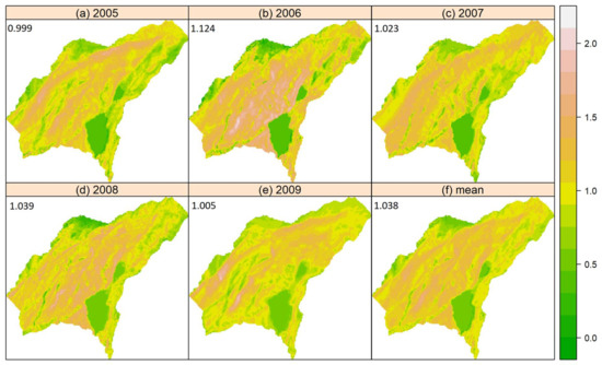
Figure 3.
The estimated standardized distribution of snow depth values (SDV) and the mean SDV in the upper left corner for (a–e) 2005 to 2009, and (f) the mean over 2005–2009.
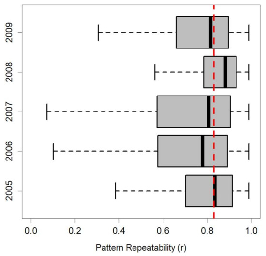
Figure 4.
The CSDP (Pearson correlation, r) computed from standardized climatological snow depth pattern and the SDV of individual years. The mean r value at 0.83 is represented by a vertical red dashed line.
4.4. Winter Season Index
The WGL winter season index was estimated from the Brooklyn Lake snow depth data (see Supplementary Materials, Figure S3) and their correlation to mean annual measured snow depth. Brooklyn Lake snow depth and the WGLW measured snow depth mean were correlated for (a) the ten measurement years (r2 = 0.75) and (b) the five calibration measurement years (r2 = 0.69) (Figure 5). The correlation between the Brooklyn Lake snow depth and the WGLW measured snow depth mean (Figure 5 was used as the winter season index since the correlation was high (r2 = 0.75). For snow depth, five of the survey dates occurred during above normal (median) years, five during below normal years, one (2011) was above the 90th percentile, and one (2012) was below the 10th percentile.
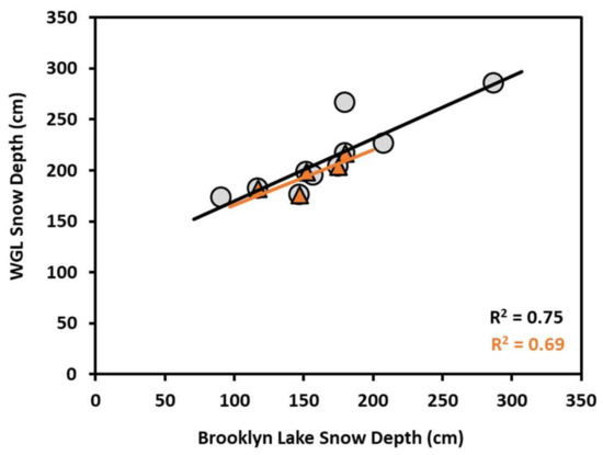
Figure 5.
The correlation between the observed or measured annual mean snow depth and the Brooklyn Lake SNOTEL snow depth for all years (2005 to 2014 in grey circles) and the calibration years (2005 to 2009 in orange triangles).
4.5. Simulated Snow Depth
The combined winter season index, the CSDP, and the measured snow depth estimated the distribution of snow with good accuracy with an average difference within 10 percent (Table 1; Figure 6). The mean simulated to observed basin snow depth difference was 8 cm, and the percent difference for the ten years was 5% (Table 1). The snow depth estimated for the record dry (2012) and wet (2011) years were captured well, with the basin mean difference of less than 10 cm and the percent difference of 5% (Table 1).
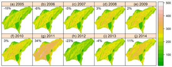
Figure 6.
The estimated distribution of snow depth for the 10 study years: (a–j) 2005 to 2014, where snow depth was sampled at approximately the time of peak snow accumulation. The percent difference from the 10-year mean snow depth (169 cm) estimated from the Brooklyn Lake SNOTEL snow depth sensor is presented in the upper left of each figure.
There was more variability in the measured snow depth than in the simulated snow depth (one standard deviation shown in the dark versus light grey boxes in Figure 7). The measurements ranged from 0 to 500+ cm, while the simulated snow depth ranged from 50 to 485 cm; minimum depth was limited in the model but maximum depth was more similar (Figure 7). Overall, the basin mean snow depth was within 10% (Figure 7; Table 1).
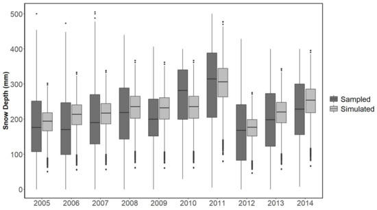
Figure 7.
Summary of the maximum, minimum, mean (black line), and standard deviation (grey bar) of the observed versus simulated snow depth.
The modeled basin mean snow depth was deeper than the measured depth (Figure 7) for the five years with the most measurements (2005 to 2009; Table 1) and in three other years (Figure 7). In the two other years (2010 and 2011), the snow depth measurements were concentrated at lower elevations (Figure 1g,i). Sampling year 2011 had a deep snowpack and, although the fewest points were collected, the mean modeled snow depth was only slightly larger than the measured snow depth (Figure 1). Sampling year 2012 also had the next fewest number of measurements but included samples at high elevations within WGLW (Figure 1i); thus, it yielded a better estimated basin mean compared to the observed mean (Figure 7). There is a positive bias of the basin mean snow depth estimated when measurements do not adequately cover the range of elevations across West Glacier Lake (Figure 1 and Figure 7), supporting the need for a model development/evaluation based on 2005 to 2009 alone, when the data are better distributed.
5. Discussion
Numerous (3382) measurements of snow depth were collected at WGLW over the 10 study years (Figure 1; Table 1). A variety of snow years were measured, including average snow years, as well as record dry (2012) and wet (2011) snow years (Figure 7), yet the standard deviation of the annual measurements had a small range, from 90 to 118 cm (Figure 1). However, due to the variation in the mean, the range of the coefficient of variation was a factor of two (0.33 to 0.63). The distribution of snow across WGLW illustrates drifted and wind scoured patterns that were controlled by persistent westerly winds [40] and topographic influences [29].
The LOP sampling method is labor intensive [20], yet it provided a robust dataset that was able to confirm a consistent snow depth distribution and repeatability (Figure 4) with the same accuracy as airborne LiDAR surveys (ALS) [10]. More advanced snow depth sampling methods, such as ALS [10,37,61], can likely spatially improve the sampling footprint (~1 m). Recent ALS efforts [62] illustrate that an increase in the temporal sampling frequency of sampling is possible [10].
The topography of WGLW dictates its distribution of snow; spatial interpolation techniques such as binary regression tree models, MLR models, geostatistical models, and GAM methods have been used to estimate snow depth and SWE distribution in complex terrain with good results [5,15,18,19,27,28,42,45,58]. Spatial modeling results indicated the GAMs provided more robust and better estimates of the basin mean snow (Figure 2), while MLR and binary regression tree models provided a decent estimate of the basin mean snow depth (Figure 2) but showed a relatively low predictive capability similar to that found by López-Moreno and Nogués-Bravo [27]. In this study, as in recent studies [27,28,46,58], the snow depth distribution modeling was performed using GAMs with topographic parameters to capture the nonlinear interactions controlling snow depth distribution. While this study utilized GAM interpolation methods, it also illustrated the methods to estimate a CSDP based on snow depth samples, how to estimate and apply a winter season index with limited snow depth samples and/or surrogate information for the CSDP to estimate a basin mean snow depth and spatial pattern.
Here, the optimal approach was chosen based on one year (2006) that had a good distribution of sampling, with almost 75% of the sampling points of the maximum number collected and a larger CV than other years in the testing period of record (Figure 1 and Table 1). Other investigations have compared interpolation methods in detail, such as Erxleben et al. [13], Hultstrand [29], and López-Moreno and Nogués-Bravo [46]. However, these only focused on one time period of data collection, though Erxleben et al. [13] examined several locations. Hultstrand [29] compared nine spatial interpolation methods for the same location (study year 2005). Such analyses are important, as the optimal model can vary depending on the location [13] or inter-annual variation in snowpack patterns, especially shallow (in this study, 2012) and deep (in this study, 2011) snow years (Figure 1, Figure 6 and Figure 7 and Table 1). Not only are snowfall quantities different in extreme snow years (Table 1), other processes have differing importance, such as sublimation, which was shown to disproportionately alter the amount of snow on the ground between 2011 and 2012 at this study site [63].
Mountain snow depth distribution is highly variable and typically controlled by meteorologic and topographic parameters [9,10,14,15]. We identified four topographic parameters that influenced snow depth distribution that were significant and consistent among the years for elevation, slope, aspect, and maximum upwind slope (Table 2; Figure S3), similar to other studies [14,56]. The slope parameter has been found to largely explain the snow distribution in steep terrain related to snow redistribution, avalanches, and as a surrogate for solar radiation [12,13,51] and northness [7,17,42,53]; in this study, slope was identified as the most significant parameter controlling snow depth distribution. Elevation is important for larger scales [24] and still relevant for more flat, forested terrain [7,13]; here, it was the second most important parameter (Table 2). Elevation and slope are correlated; where there is a larger elevation gradient across a study domain, especially a small domain, i.e., where measurements are meters to tens of meters apart (rather than kilometers, such as in Fassnacht et al. [24]), the slopes are steeper. Water ponding [44] is a partial surrogate for the topographic position index, that has been used as an indicator of the distribution of snow depth [19]; here, it was minimally relevant (Table 2).
Where large elevational differences exist, elevation explains much of the snow distribution [5,12,13,24], or in some cases such as WGLW (Table 2), limited elevational differences [7]. Aspect was the second most significant variable. The maximum upwind slope has been found to largely explain the snow distribution in areas of topography that have consistent prevailing winds [3,5,14,19,55].
We modeled snow depth distribution for five calibration years (2005 to 2009) with a high degree of accuracy and repeatability (r = 0.83). These five years were used to estimate a CSDP for WGLW. To characterize the winter season in regard to precipitation magnitude, we developed a winter season index for WGLW based on the nearby Brooklyn Lake SNOTEL station data. Then, the CSDP and winter season index were used to estimate the at or near peak distribution of snow depth with a relatively high confidence for years with fewer measurements. The estimated basin mean snow depth represented the snow depth measurements well (r2 = 0.75), but as is typical with many models, it did not capture the range of snow depth measurements as well (Figure 7). To estimate snow depth for years with limited or no snow depth samples, the winter season index, based on Brooklyn Lake’s snow depth near peak accumulation, can be used to estimate the mean snow depth at the WGLW basin (Figure 5) and the CSDP (Figure 3f) can be applied to estimate the snow depth spatial distribution when snow depth data are not collected. However, when direct samples of snow depth are available then, GAMs can successfully model snow depth distribution and SWE using topographic indicators to capture the nonlinear interactions controlling snow depth distribution
Hydrological applications require the snowpack to be characterized in terms of SWE rather than snow depth [2,11,24]. Measuring and/or estimating snow density and SWE requires substantially more effort than snow depth sampling [3,64]. It has been observed that snow depth is highly variable compared to depth integrated snowpack density [3,64], and SWE is strongly correlated to snow depth [12,64]. Therefore, much fewer density measurements are needed to capture the variability in density, and thus SWE, than snow depth. Thus, good estimates of the distribution of snow depth (Figure 6 and Figure 7) with an adequate number of density measurements [64] can be used to estimate SWE.
Under a changing climate, snow distribution for a given date, such as 1 April, may be less repeatable during water years where deviations from normal temperature and precipitation influence the amount and precipitation phase [10]. Although snow depth for a given date may change, the underlying interaction of topography and meteorological patterns that influence snow distribution should not change. This implies that the modeled CSDP and winter season index methods discussed should be applicable to estimate snow depth distribution in WGLW under future climate conditions.
This study helps to advance the science by estimating snow distributions within a small watershed using CSDP and WSI methodology over a 10-year period; it is important to highlight some of the limitations and potential future investigations. The limitations of this study are that it is focused on a high elevation, windy environment. The LOP snow depth sampling method was used, which is only relevant for small basins. The accuracy of the CSDP is influenced by the GAM interpolation methods and the 5 m. Future research that is focused on simulating the processes driving snow distribution or the development of CSDP at fine resolution (1 m), based on field measurements and ALS, may be particularly useful for model evaluations [10], to investigate snow distribution repeatability [16] and to quantify uncertainty.
6. Conclusions
Ten years of snow depth measurements at or on the peak were analyzed and showed a consistent snow depth distribution over the period of measurements. A method was illustrated to map the distribution of snow depth. A general additive model (GAM) was shown to be statistically superior to a binary regression tree or multiple linear regression approaches. The GAM interpolation was able capture the nonlinear nature of the correlation between snow depth and the topographic parameters. The parameters that were significant predictors of the distribution of snow depth were elevation, slope, aspect, and maximum upwind slope. The GAM was used with topographic parameters to estimate a climatological snow depth pattern which was scaled based on a winter season index with high accuracy, both quantitatively and qualitatively.
Supplementary Materials
The following are available online at https://www.mdpi.com/article/10.3390/atmos13010003/s1, Figure S1: Significant topographic parameters elevation (a,e); slope (b,f); aspect (c,g); and maximum upwind slope (d,h) non-linear relationships to snow depth for sample years 2006 and 2008, Figure S2: The strongest correlation for all topographic parameters and multi-year models (r = 0.29) for the residuals from the multi-year model omitting 2006 versus elevation. All other residual versus topographic parameter correlations (Table 2) were less than 0.19. Figure S3: Snow survey dates plotted on top of snow depth data from the Brooklyn Lake SNOTEL site for available years of data: 2004 through 2021. The gold symbols are the survey dates and associated SNOTEL date values.
Author Contributions
Methodology, D.M.H. and S.R.F.; software, D.M.H.; formal analysis, D.M.H.; investigation, D.M.H., S.R.F., J.D.S., and C.A.H.; resources, D.M.H.; data curation, D.M.H.; writing—original draft preparation, D.M.H. and S.R.F.; writing—review and editing, D.M.H., S.R.F., J.D.S., and C.A.H.; supervision, S.R.F. and J.D.S. All authors have read and agreed to the published version of the manuscript.
Funding
This research did not have any direct funding.
Institutional Review Board Statement
Not applicable.
Informed Consent Statement
Not applicable.
Data Availability Statement
Hourly meteorological data of air temperature, solar radiation, relative humidity, scalar wind speed, wind direction, soil temperature, and wet–dry sensor measurements from the Glacier Lakes Ecosystem Experiments Site (GLEES), in the Snowy Range near Centennial, Wyoming [65]. The snow depth field sample dataset is currently in the formal data review process [66].
Acknowledgments
Numerous individuals assisted with field work and the collection of the data at the Glacier Lakes Ecosystems Experiments Site over the 10 years; we thank them for their hard work. Robert Musselman and John Korfmacher of the Rocky Mountain Research Station (RMRS) provided logistical support, access to the site in the winter, and access to the data; we are grateful for this support. We thank the two anonymous reviewers provided good insight.
Conflicts of Interest
The authors declare no conflict of interest.
Appendix A. Topographic Parameters
This Appendix summarizes the topographic parameters and their derivation.
Appendix A.1. Elevation
Point elevation was extracted directly from the 5 m digital elevation model (DEM). This DEM was then used to generate the snow depth maps.
Appendix A.2. Slope
Slope was calculated from the DEM using the Spatial Analyst Tool in ArcGIS® [67]. This function calculates the maximum rate of change between each cell and the surrounding cell. Each cell in the output raster has a slope; a lower slope corresponds to flatter terrain while a higher slope represents steeper terrain.
Appendix A.3. Aspect
Aspect was calculated from the DEM using the Spatial Analyst Tool in ArcGIS® [67]. This function identifies the steepest downslope direction from each cell to its neighbors. Each cell in the output slope raster is a categorical value representing the direction that the cell’s slope faces.
Appendix A.4. Northness
Northness was calculated as the product of the sine of the slope and the cosine of the aspect [5].
Appendix A.5. Solar Radiation
The Solar Analyst is an ArcGIS® extension that computes various components of solar radiation following the routine of Fu and Rich [68] using the elevation, slope, and aspect rasters summarized in Section A.1, Section A.2 and Section A.3. Here, the clear sky solar radiation was computed to consider the shading from surrounding hillslopes.
Appendix A.6. Ponding
Ponded water is the depth (m) of any surface depression compared to the surrounding cells and is determined from the DEM [44]. Ponding depth was computed as the difference from the 5 m DEM and the filled (FILL function in ArcGIS®) or modified block-filter average smoothed DEM.
Appendix A.7. Maximum Upslope Wind
The maximum upwind slope parameter (Sx), defined by Winstral and Marks [56], is
where A is the azimuth of the search direction, dmax is lateral search distance, (xi,yi) are the coordinates of the cell of interest, and (xv,yv) are the set of cell coordinates located along the line segment defined by (xi,yi), A, and dmax. Negative Sx values indicate exposure relative to the shelter-defining pixel (i.e., the cell of interest is higher than the shelter defining pixel).
Averaging the Sx value across the upwind direction is shown to be more robust to both natural and systematic deviations [56]. The mean maximum upwind slope parameter (), defined by Winstral and Marks [56], is
where A1 and A2 define the outer limits of the upwind directions, bisects A1 and A2, and nv is the number of search vectors in the window defined by A1 and A2.
Appendix B. Interpolation Models
Appendix B.1. Binary Regression Tree
BRT models estimate dependent variables from a group of independent variables (here parameters, since they are constant over time) in a non-linear hierarchical manner through a series of binary decisions [69]. Snow depth data are often related to independent variables in a non-linear and hierarchical manner [5,13]. Binary recursive partitioning bin together increasing homogenous subsets of data. Detailed explanations of BRT fitting, pruning, and cross-validation are found in Balk and Elder [44], Breiman et al. [69], and Elder et al. [70]. The optimal combination of topographic parameters within a specific BRT model was selected based on the lowest deviance and highest coefficient of determination (r2) [71].
Appendix B.2. Multiple Linear Regression
MLR models can estimate the non-linear correlations between a dependent variable and one or more independent variables, and thus go beyond traditional linear regression models. The MLR model approach was used for snow depth versus topographic parameters. The initial parameter was selected based on the largest correlation with snow depth. The stepwise addition of parameters continued until the addition/removal of new variables no longer increased the correlation coefficient by a specific amount, as per the procedure of Fassnacht et al. [24].
Appendix B.3. Generalized Additive Model
GAM models go beyond linear regression models by applying non-parametric smoothing functions to each predictor and additively calculating the component response [27,72]. GAM models can incorporate non-Gaussian error distributions and non-linear correlations between response and predictor variables.
References
- Hammond, J.C.; Saavedra, F.A.; Kampf, S.K. How Does Snow Persistence Relate to Annual Streamflow in Mountain Watersheds of the Western U.S. With Wet Maritime and Dry Continental Climates? Water Resour. Res. 2018, 54, 2605–2623. [Google Scholar] [CrossRef]
- McKay, G.A.; Gray, D.M. The Distribution of the Snow Cover. In Handbook of Snow: Principles Processes, Management and Use; Gray, D.M., Hale, D., Eds.; Pergamon Press: Willowdale, ON, Canada, 1981; pp. 153–190. [Google Scholar]
- Elder, K.; Dozier, J.; Michaelsen, J. Snow accumulation and distribution in an Alpine Watershed. Water Resour. Res. 1991, 27, 1541–1552. [Google Scholar] [CrossRef]
- Cline, D.; Pomeroy, J.W.; Gray, D.M. Snowcover Accumulation, Relocation and Management. Arct. Alp. Res. 1998, 30, 314. [Google Scholar] [CrossRef]
- Molotch, N.P.; Colee, M.T.; Bales, R.C.; Dozier, J. Estimating the spatial distribution of snow water equivalent in an alpine basin using binary regression tree models: The impact of digital elevation data and independent variable selection. Hydrol. Process. 2005, 19, 1459–1479. [Google Scholar] [CrossRef]
- Elder, K.; Cline, D.; Liston, G.E.; Armstrong, R. NASA Cold Land Processes Experiment (CLPX 2002/03): Field Measurements of Snowpack Properties and Soil Moisture. J. Hydrometeorol. 2009, 10, 320–329. [Google Scholar] [CrossRef]
- Fassnacht, S.R.; Brown, K.S.J.; Blumberg, E.J.; López-Moreno, J.I.; Covino, T.P.; Kappas, M.; Huang, Y.; Leone, V.; Kashipazha, A.H. Distribution of snow depth variability. Front. Earth Sci. 2018, 12, 683–692. [Google Scholar] [CrossRef]
- Mott, R.; Vionnet, V.; Grünewald, T. The Seasonal Snow Cover Dynamics: Review on Wind-Driven Coupling Processes. Front. Earth Sci. 2018, 6, 1–25. [Google Scholar] [CrossRef]
- Elder, K.; Dozier, J. Improving Methods for Measurement and Estimation of Snow Storage in an Alpine Watershed; IAHS Publication: Wallingford, UK, 1990; Volume 193, pp. 147–156. [Google Scholar]
- Pflug, J.M.; Lundquist, J.D. Inferring Distributed Snow Depth by Leveraging Snow Pattern Repeatability: Investigation Using 47 Lidar Observations in the Tuolumne Watershed, Sierra Nevada, California. Water Resour. Res. 2020, 56, 1–17. [Google Scholar] [CrossRef]
- Meiman, J.R. Snow accumulation related to elevation, aspect, and forest canopy. In Proceedings of the Snow Hydrology Workshop Seminar, Fredericton, NB, Canada, 28–29 February 1968; pp. 35–47. [Google Scholar]
- Elder, K.; Rosenthal, W.; Davis, R. Estimating the spatial distribution of snow water equivalent in a montane watershed. Hydrol. Process. 1998, 12, 1793–1808. [Google Scholar] [CrossRef]
- Erxleben, J.; Elder, K.; Davis, R. Comparison of spatial interpolation methods for estimating snow distribution in the Colorado Rocky Mountains. Hydrol. Process. 2002, 16, 3627–3649. [Google Scholar] [CrossRef]
- Winstral, A.; Elder, K.; Davis, R.E. Spatial Snow Modeling of Wind-Redistributed Snow Using Terrain-Based Parameters. J. Hydrometeorol. 2002, 3, 524–538. [Google Scholar] [CrossRef]
- Erickson, T.A.; Williams, M.W.; Winstral, A. Persistence of topographic controls on the spatial distribution of snow in rugged mountain terrain, Colorado, United States. Water Resour. Res. 2005, 41. [Google Scholar] [CrossRef]
- Sturm, M.; Wagner, A.M. Using repeated patterns in snow distribution modeling: An Arctic example. Water Resour. Res. 2010, 46, 12549. [Google Scholar] [CrossRef]
- Alarcón, J.L.; De Luco, D.F.; Garcia-Gonzalez, R.; García-Serrano, A.; Herrero, J. Primera Reunión sobre el rebeco cantábrico y el sarrio pirenaico. Benasque (Huesca, España), 20–22 de mayo de 2011. Pirineos 2011, 166, 155–177. [Google Scholar] [CrossRef][Green Version]
- Grünewald, T.; Stötter, J.; Pomeroy, J.W.; Dadic, R.; Baños, I.M.; Marturià, J.; Spross, M.; Hopkinson, C.; Burlando, P.; Lehning, M. Statistical modelling of the snow depth distribution in open alpine terrain. Hydrol. Earth Syst. Sci. 2013, 17, 3005–3021. [Google Scholar] [CrossRef]
- Revuelto, J.; López-Moreno, J.I.; Azorin-Molina, C.; Vicente-Serrano, S.M. Topographic control of snowpack distribution in a small catchment in the central Spanish Pyrenees: Intra- and inter-annual persistence. Cryosphere 2014, 8, 1989–2006. [Google Scholar] [CrossRef]
- Grayson, R.B.; Bloschl, G.; Western, A.W.; McMahon, T.A. Advances in the use of observed spatial patterns of catchment hydrological response. Adv. Water Resour. 2002, 25, 1313–1334. [Google Scholar] [CrossRef]
- Fassnacht, S.R.; Deitemeyer, D.C.; Venable, N.B.H. Capitalizing on the daily time step of snow telemetry data to model the snowmelt components of the hydrograph for small watersheds. Hydrol. Process. 2014, 28, 4654–4668. [Google Scholar] [CrossRef]
- Godsey, S.E.; Kirchner, J.; Tague, C.L. Effects of changes in winter snowpacks on summer low flows: Case studies in the Sierra Nevada, California, USA. Hydrol. Process. 2013, 28, 5048–5064. [Google Scholar] [CrossRef]
- Carroll, R.W.H.; Deems, J.S.; Niswonger, R.; Schumer, R.; Williams, K.H. The Importance of Interflow to Groundwater Recharge in a Snowmelt-Dominated Headwater Basin. Geophys. Res. Lett. 2019, 46, 5899–5908. [Google Scholar] [CrossRef]
- Fassnacht, S.R.; Dressler, K.A.; Bales, R.C. Snow water equivalent interpolation for the Colorado River Basin from snow telemetry (SNOTEL) data. Water Resour. Res. 2003, 39, 1208. [Google Scholar] [CrossRef]
- Zheng, Z.; Kirchner, P.B.; Bales, R.C. Topographic and vegetation effects on snow accumulation in the southern Sierra Nevada: A statistical summary from lidar data. Cryosphere 2016, 10, 257–269. [Google Scholar] [CrossRef]
- Gleason, K.; Nolin, A.W.; Roth, T.R. Developing a representative snow-monitoring network in a forested mountain watershed. Hydrol. Earth Syst. Sci. 2017, 21, 1137–1147. [Google Scholar] [CrossRef]
- López-Moreno, J.I.; Nogués-Bravo, D. A generalized additive model for the spatial distribution of snowpack in the Spanish Pyrenees. Hydrol. Process. 2005, 19, 3167–3176. [Google Scholar] [CrossRef]
- Moreno, J.I.L.; Latron, J.; Lehmann, A. Effects of sample and grid size on the accuracy and stability of regression-based snow interpolation methods. Hydrol. Process. 2009, 24, 1914–1928. [Google Scholar] [CrossRef]
- Hultstrand, D.M. Geostatistical Methods for Estimating Snowmelt Contribution to the Seasonal Water Balance in an Alpine Watershed. Master’s Thesis, Colorado State University, Fort Collins, CO, USA, 2006. Available online: https://hdl.handle.net/10217/233658 (accessed on 27 October 2021).
- Boustead, B.E.M.; Hilberg, S.D.; Shulski, M.D.; Hubbard, K.G. The Accumulated Winter Season Severity Index (AWSSI). J. Appl. Meteorol. Clim. 2015, 54, 1693–1712. [Google Scholar] [CrossRef]
- Vögeli, C.; Lehning, M.; Wever, N.; Bavay, M. Scaling Precipitation Input to Spatially Distributed Hydrological Models by Measured Snow Distribution. Front. Earth Sci. 2016, 4, 4. [Google Scholar] [CrossRef]
- Cerruti, B.J.; Decker, S.G. The Local Winter Storm Scale: A Measure of the Intrinsic Ability of Winter Storms to Disrupt Society. Bull. Am. Meteorol. Soc. 2011, 92, 721–737. [Google Scholar] [CrossRef][Green Version]
- Tarboton, D.G.; Luce, C.H. Utah Energy Balance Snow Accumulation Model (UEB)—Computer Model Technical Description and Users Guide; Utah Water Research Laboratory and USDA Forest Service Intermountain Research Station: Logan, UT, USA, 2006; p. 64. [Google Scholar]
- Bloschl, G.; Grayson, R. Spatial Observations and Interpolation. In Spatial Pattern in Catchment Hydrology: Observations and Modeling; Grayson, R., Bloschl, G., Eds.; Cambridge University Press: Cambridge, UK, 2001; pp. 17–50. [Google Scholar]
- Hiemstra, C.A.; Liston, G.E.; Reiners, W.A. Observing, modelling, and validating snow redistribution by wind in a Wyoming upper treeline landscape. Ecol. Model. 2006, 197, 35–51. [Google Scholar] [CrossRef]
- Wooldridge, G.L.; Musselman, R.C.; Sommerfeld, R.A.; Fox, D.G.; Connell, B.H. Mean Wind Patterns and Snow Depths in an Alpine-Subalpine Ecosystem as Measured by Damage to Coniferous Trees. J. Appl. Ecol. 1996, 33, 100. [Google Scholar] [CrossRef][Green Version]
- Deems, J.S.; Fassnacht, S.R.; Elder, K.J. Interannual Consistency in Fractal Snow Depth Patterns at Two Colorado Mountain Sites. J. Hydrometeorol. 2008, 9, 977–988. [Google Scholar] [CrossRef]
- López-Moreno, J.I.; Revuelto, J.; Fassnacht, S.; Azorin-Molina, C.; Vicente-Serrano, S.M.; Morán-Tejeda, E.; Sexstone, G.A. Snowpack variability across various spatio-temporal resolutions. Hydrol. Process. 2014, 29, 1213–1224. [Google Scholar] [CrossRef]
- Musselman, R.C. The Glacier Lakes Ecosystem Experiments Site. Rocky Mountain Forest and Range Experiment Station, General Technical Report RM-249; U.S. Dept. of Agriculture: Fort Collins, CO, USA, 1994; p. 94. [Google Scholar]
- Korfmacher, J.L.; Hultstrand, D.M. Glacier Lakes Ecosystem Experiments Site Hourly Meteorology Tower Data; Rocky Mountain Research Station, U.S.; Forest Service, U.S.; Department of Agriculture: Fort Collins, CO, USA, 2006. [Google Scholar]
- Hultstrand, D.M.; Fassnacht, S.R.; Stednick, J.D. Geostatistical methods for estimating snowmelt contribution to the alpine water balance. In Proceedings of the Annual Western Snow Conference, Las Cruces, NM, USA, 17–20 April 2006; Volume 74, pp. 149–154. [Google Scholar]
- Fassnacht, S.; López-Moreno, J.; Toro, M.; Hultstrand, D. Mapping snow cover and snow depth across the Lake Limnopolar watershed on Byers Peninsula, Livingston Island, Maritime Antarctica. Antarct. Sci. 2013, 25, 157–166. [Google Scholar] [CrossRef][Green Version]
- Cline, D.; Elder, K.; Bales, R.C. Scale effects in a distributed snow water equivalence and snowmelt model for mountain basins. Hydrol. Process. 1998, 112, 1527–1536. [Google Scholar] [CrossRef]
- Lapen, D.R.; Martz, L.W. An investigation of the spatial association between snow depth and topography in a Prairie agricultural landscape using digital terrain analysis. J. Hydrol. 1996, 184, 227–298. [Google Scholar] [CrossRef]
- Balk, B.; Elder, K. Combining binary regression tree and geostatistical methods to estimate snow distribution in a mountain watershed. Water Resour. Res. 2000, 36, 13–26. [Google Scholar] [CrossRef]
- López-Moreno, J.I.; Nogués-Bravo, D. Interpolating snow depth data: A comparison of methods. Hydrol. Process. 2006, 20, 2217–2232. [Google Scholar] [CrossRef]
- Musselman, R.C. (Rocky Mountain Research Station, Fort Collins, CO, USA). Personal communication, 2004.
- DeWalle, D.R.; Rango, A. Principles of Snow Hydrology; Cambridge University Press: Cambridge, UK, 2008; p. 428. [Google Scholar] [CrossRef]
- Barry, R.G. Mountain Weather and Climate, 2nd ed.; Routledge: New York, NY, USA, 1992; p. 402. [Google Scholar]
- Roe, G.H. Orographic Precipitation. Annu. Rev. Earth Planet Sci. 2005, 33, 645–671. [Google Scholar] [CrossRef]
- McClung, D.; Schaerer, P. The Avalanche Handbook, 3rd ed.; The Mountaineers: Seattle, WA, USA, 2006; p. 272. [Google Scholar]
- Deems, J.S. Topographic Effects on the Spatial and Temporal Patterns of Snow Temperature Gradients in a Mountain Snowpack. Master’s Thesis, Montana State University, Bozeman, MT, USA, 2002. [Google Scholar]
- Meromy, L.; Molotch, N.P.; Link, T.E.; Fassnacht, S.R.; Rice, R. Subgrid variability of snow water equivalent at operational snow stations in the western USA. Hydrol. Process. 2013, 27, 2383–2400. [Google Scholar] [CrossRef]
- Whiting, J.M.; Kiss, J. Integration of Digital Terrain Models into Ground Based Snow and Runoff Measurements; IAHS Publication: Wallingford, UK, 1987; Volume 166, pp. 375–387. [Google Scholar]
- Luce, C.H.; Tarboton, D.G.; Cooley, K.R. The influence of the spatial distribution of snow on basin-averaged snowmelt. Hydrol. Process. 1998, 12, 1671–1683. [Google Scholar] [CrossRef]
- Winstral, A.; Marks, D. Simulating wind fields and snow redistribution using terrain-based parameters to model snow accumulation and melt over a semi-arid mountain catchment. Hydrol. Process. 2002, 16, 3585–3603. [Google Scholar] [CrossRef]
- Marofi, S.; Tabari, H.; Abyaneh, H.Z. Predicting Spatial Distribution of Snow Water Equivalent Using Multivariate Non-linear Regression and Computational Intelligence Methods. Water Resour. Manag. 2011, 25, 1417–1435. [Google Scholar] [CrossRef]
- Björk, P. Modelling the spatial variability of maximum mountain snow depth in Northern Norway. Nord. Geogr. Publ. 2016, 45, 81–88. [Google Scholar]
- Willmott, C.T. Some comments on the evaluation of model performance. Bull. Am. Meteorol. Soc. 1982, 63, 1309–1313. [Google Scholar] [CrossRef]
- Hastings, W.K. Monte Carlo sampling methods using Markov chains and their applications. Biometrika 1970, 57, 97–109. [Google Scholar] [CrossRef]
- Deems, J.S.; Painter, T.H.; Finnegan, D.C. Lidar measurement of snow depth: A review. J. Glaciol. 2013, 59, 467–479. [Google Scholar] [CrossRef]
- Painter, T.H.; Berisford, D.F.; Boardman, J.W.; Bormann, K.J.; Deems, J.; Gehrke, F.; Hedrick, A.; Joyce, M.; Laidlaw, R.; Marks, D.; et al. The Airborne Snow Observatory: Fusion of scanning lidar, imaging spectrometer, and physically-based modeling for mapping snow water equivalent and snow albedo. Remote Sens. Environ. 2016, 184, 139–152. [Google Scholar] [CrossRef]
- Hultstrand, D.M.; Fassnacht, S.R. The sensitivity of snowpack sublimation estimates to instrument and measurement uncertainty perturbed in a Monte Carlo framework. Front. Earth Sci. 2018, 12, 728–738. [Google Scholar] [CrossRef]
- López-Moreno, J.; Fassnacht, S.; Heath, J.; Musselman, K.; Revuelto, J.; Latron, J.; Morán-Tejeda, E.; Jonas, T. Small scale spatial variability of snow density and depth over complex alpine terrain: Implications for estimating snow water equivalent. Adv. Water Resour. 2013, 55, 40–52. [Google Scholar] [CrossRef]
- Korfmacher, J.L.; Hultstrand, D.M.; Doebley, V.T. Glacier Lakes Ecosystem Experiments Site (GLEES) Hourly Meteorology Tower Data, 2nd ed.; Forest Service Research Data Archive: Washington, DC, USA, 2017. [Google Scholar]
- Hultstrand, D.M.; Fassnacht, S.R.; Stednick, J.D. GLEES (Glacier Lakes Ecosystem Experiments Site) Snow Depth Data Measured Annually at Peak Accumulation from 2005 to 2014. PANGAEA submitted for publication (December 2021). Available online: https://issues.pangaea.de/browse/PDI-30542 (accessed on 15 December 2021).
- ArcGIS Desktop: Release 10.8; Environmental Systems Research Institute (ESRI): Redlands, CA, USA, 2020.
- Fu, P.; Rich, P.M. The Solar Analyst 1.0 User Manual; Helios Environmental Modeling Institute LLC (HEMI): Douglas, KS, USA, 2000. [Google Scholar]
- Breiman, L.; Friedman, J.; Olsen, R.; Stone, C. Classification and Regression Trees; Wadsworth and Brooks: Pacific Grove, CA, USA, 1984; p. 358. [Google Scholar]
- Elder, K.; Michaelson, J.; Dozier, J. Small Basin Modeling of Snow Water Equivalence Using Binary Regression Tree Methods; IAHS Publication: Wallingford, UK, 1995; Volume 228, pp. 129–139. [Google Scholar]
- Peart, N. Something for Nothing. In 2112; Brown, T., Ed.; Anthem Records: Toronto, ON, Canada, 1976; track 6. [Google Scholar]
- Hastie, T.; Tibshirani, R. Generalised additive model: Some applications. J. Am. Stat. Assoc. 1987, 82, 371–386. [Google Scholar] [CrossRef]


Publisher’s Note: MDPI stays neutral with regard to jurisdictional claims in published maps and institutional affiliations. |
© 2021 by the authors. Licensee MDPI, Basel, Switzerland. This article is an open access article distributed under the terms and conditions of the Creative Commons Attribution (CC BY) license (https://creativecommons.org/licenses/by/4.0/).