
Analysis of a Short-Term and a Seasonal Precipitation Forecast over Kenya

 , , , ,
Abstract
1. Introduction
2. Materials and Methods
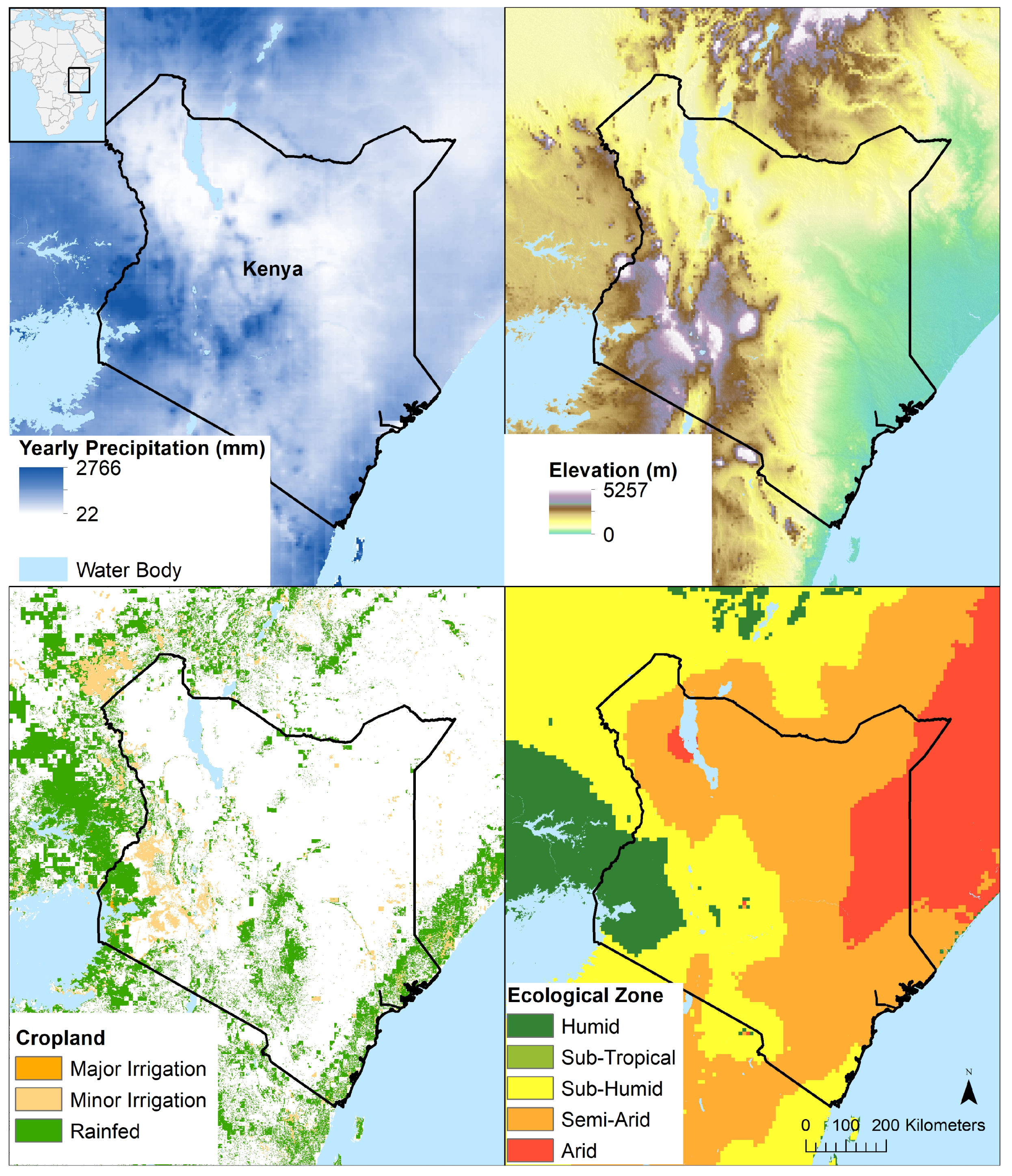
2.1. Study Area and Period
2.2. Data
2.3. Methods
2.3.1. Onset Date
2.3.2. Seasonal Forecast
3. Results
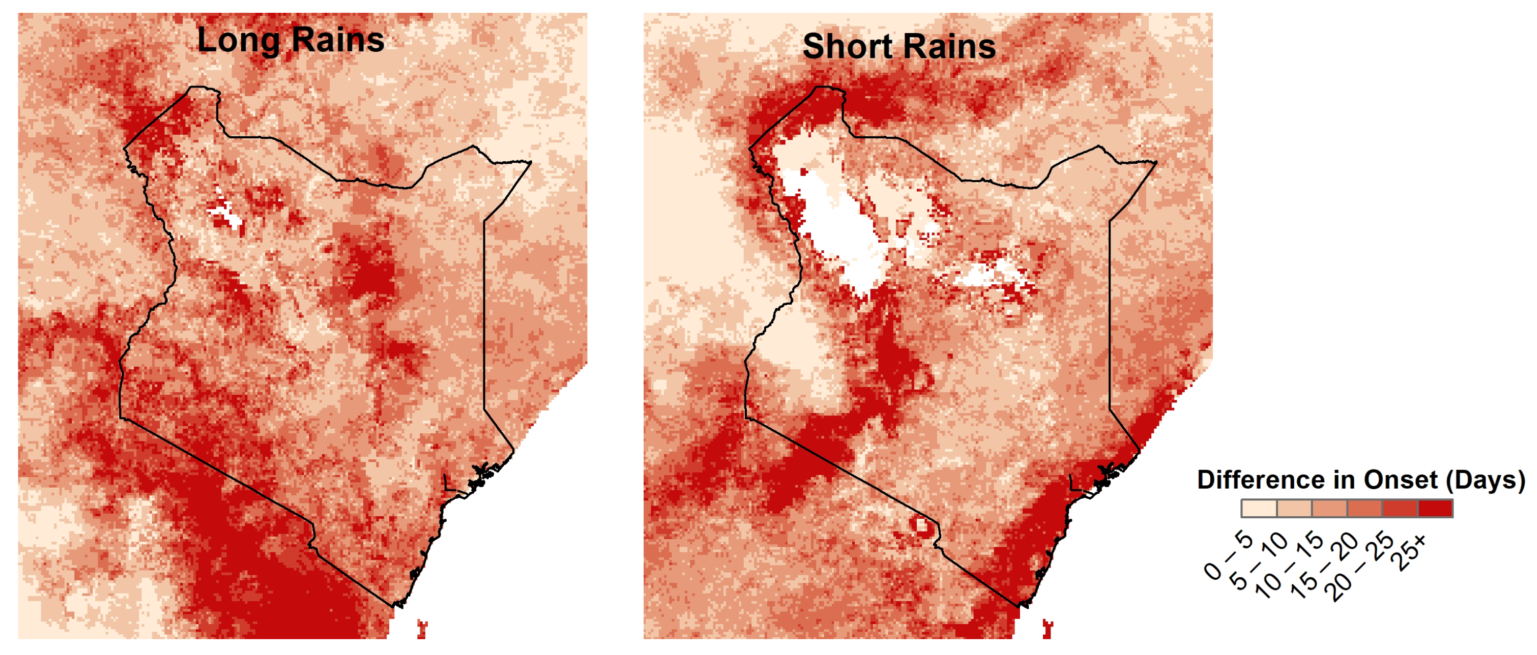
3.1. Onset Date
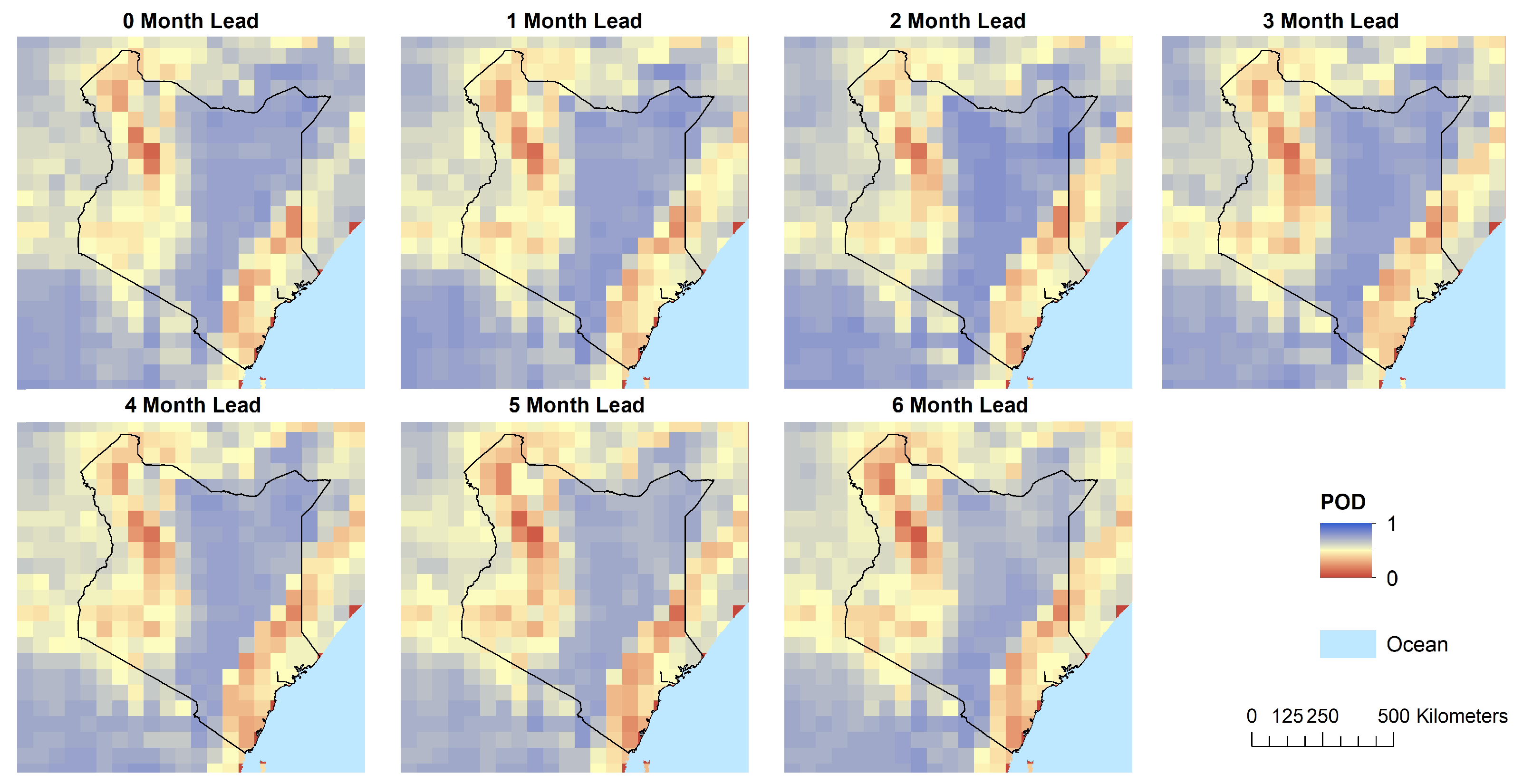
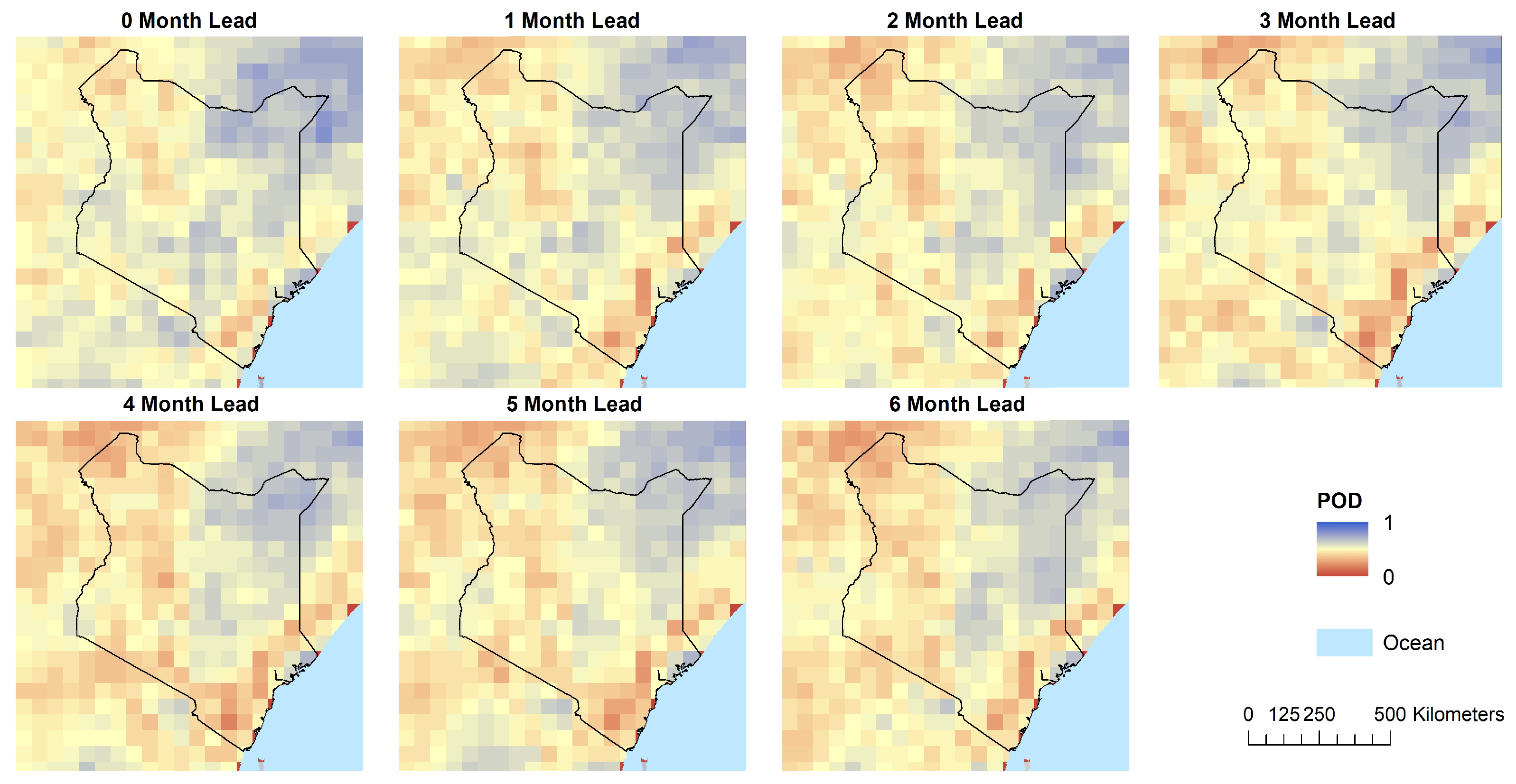
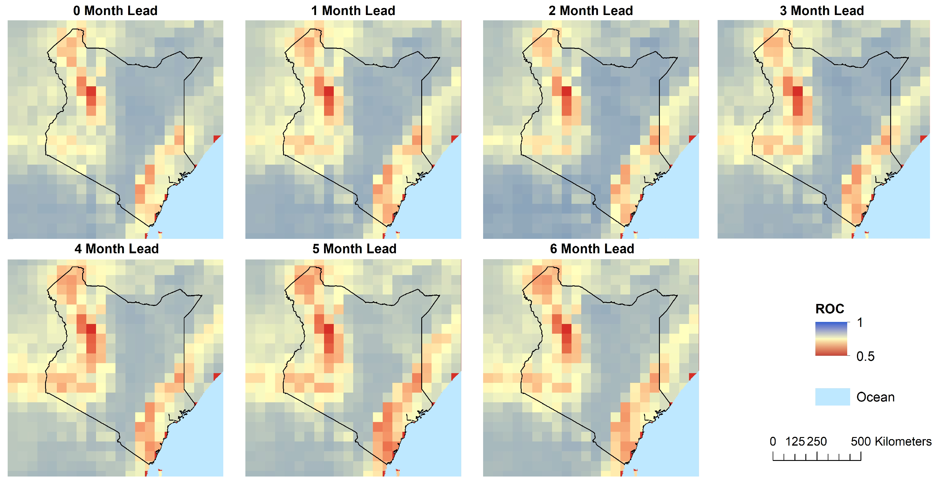
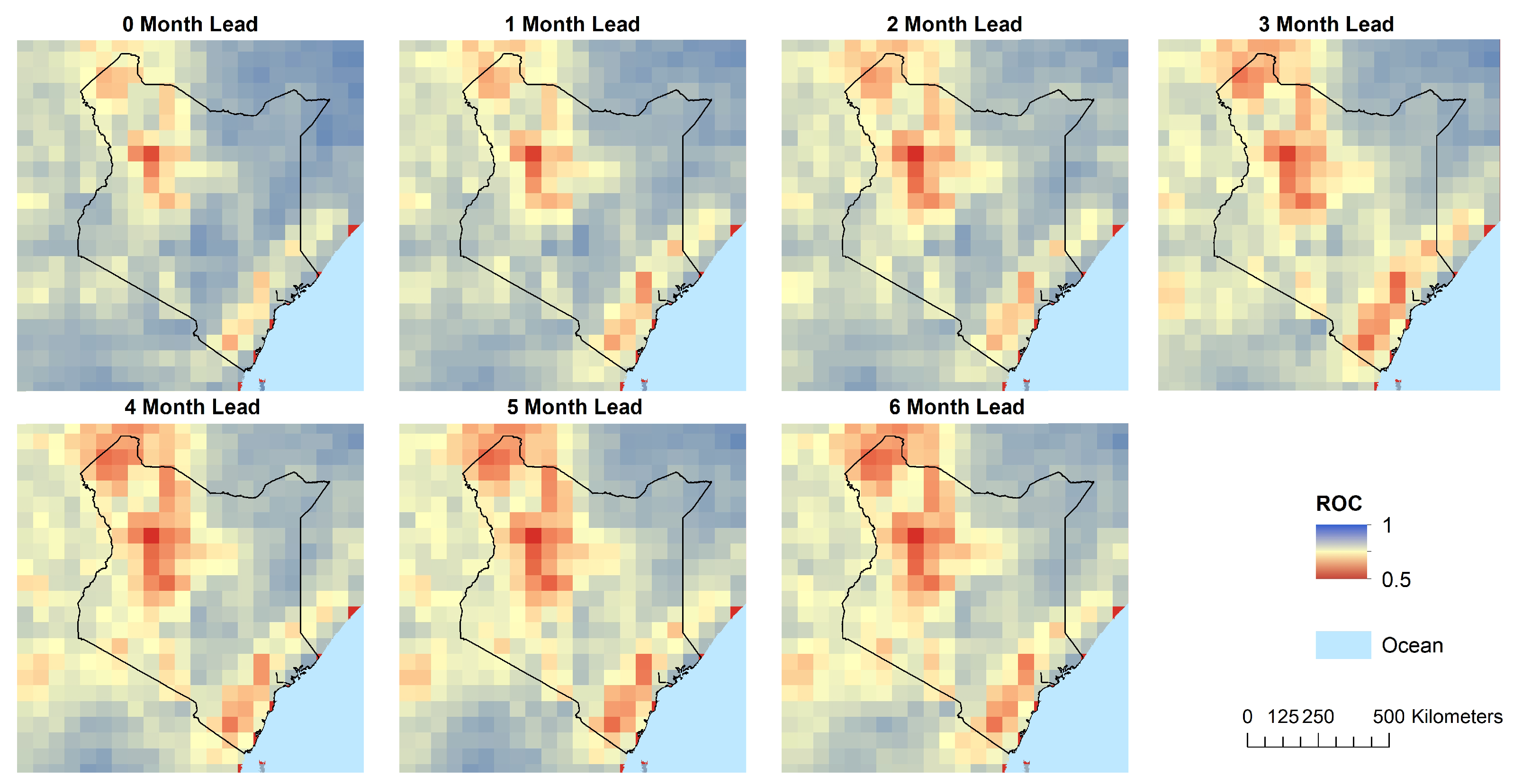
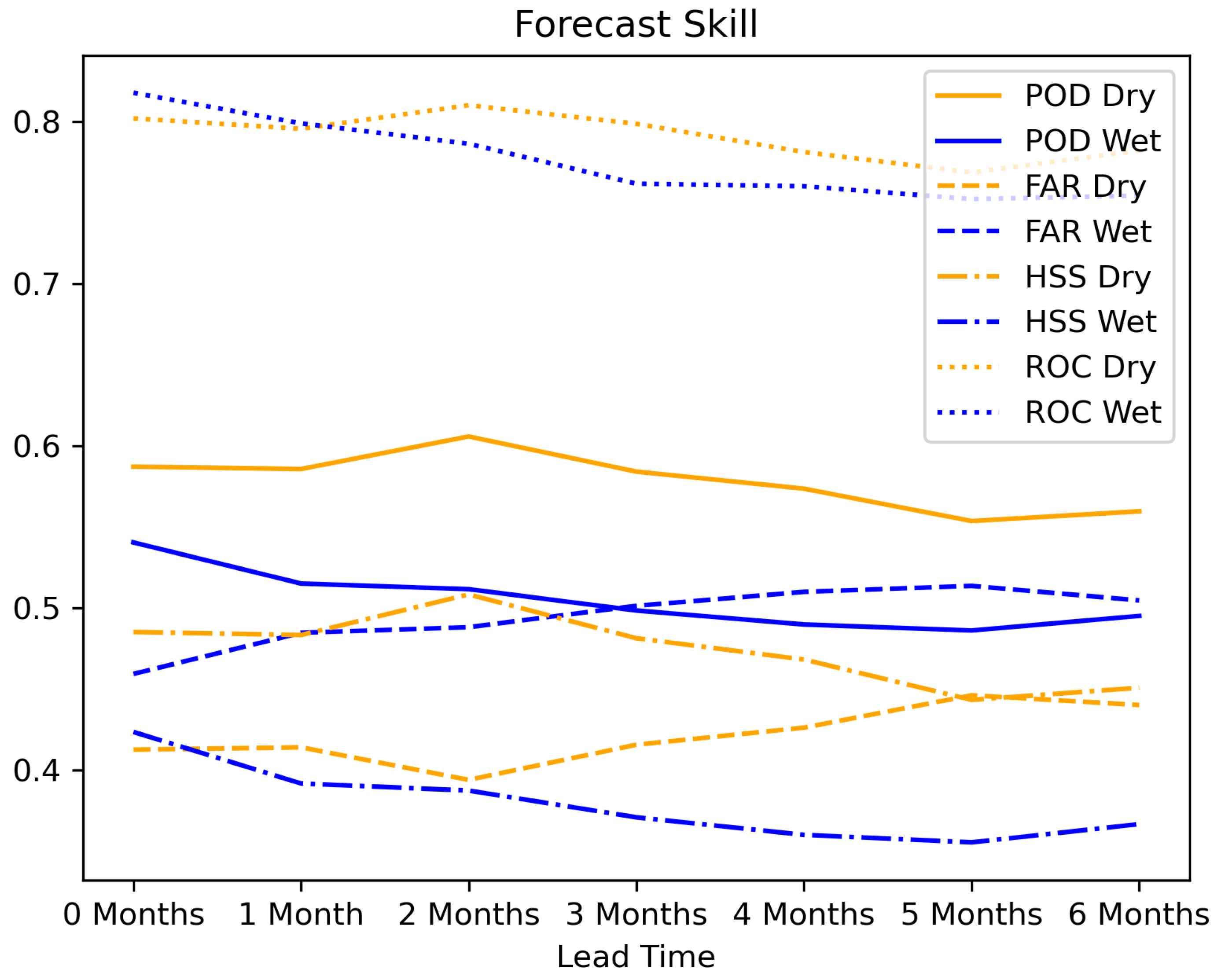
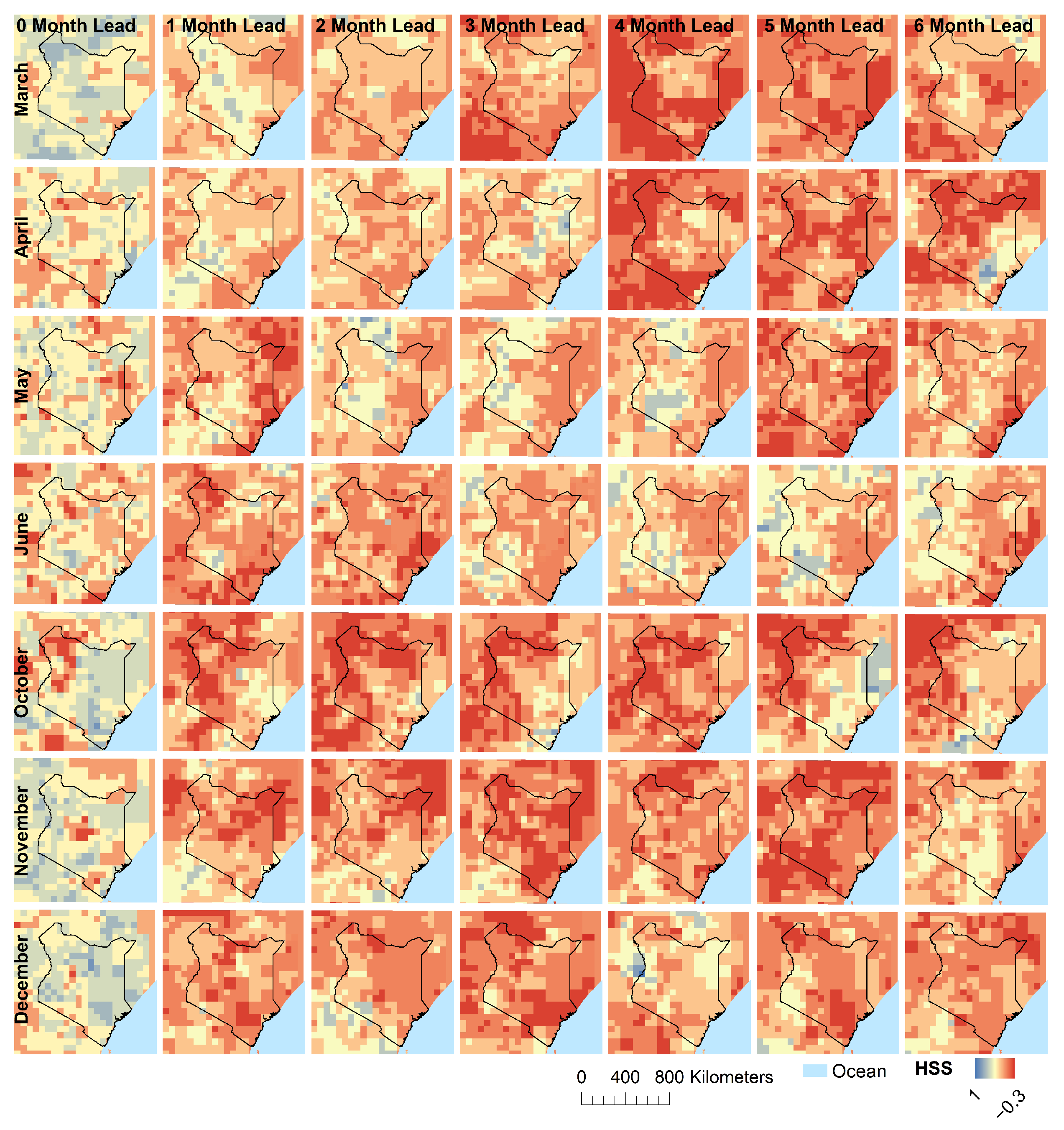
3.2. Seasonal Forecast
4. Discussion
4.1. Onset Date
4.2. Seasonal Forecast
5. Conclusions
Author Contributions
Funding
Institutional Review Board Statement
Informed Consent Statement
Acknowledgments
Conflicts of Interest
References
- Food and Agriculture Organization of the United Nations. The Agriculture Sector in Kenya. n.d. Available online: http://www.fao.org/kenya/fao-in-kenya/kenya-at-a-glance/en/ (accessed on 1 June 2021).
- Food and Agriculture Organization of the United Nations. Kenya. 2018. Available online: http://www.fao.org/faostat/en/#country/114 (accessed on 3 June 2021).
- Nicholson, S.E. Climate and climatic variability of rainfall over eastern Africa. Rev. Geophys. 2017, 55, 590–635. [Google Scholar] [CrossRef]
- Hastenrath, S.; Polzin, D.; Mutai, C. Circulation mechanisms of Kenya rainfall anomalies. J. Clim. 2011, 24, 404–412. [Google Scholar] [CrossRef]
- Hastenrath, S. Circulation mechanisms of climate anomalies in East Africa and the equatorial Indian Ocean. Dyn. Atmos. Ocean. 2007, 43, 25–35. [Google Scholar] [CrossRef]
- Hastenrath, S.; Polzin, D.; Camberlin, P. Exploring the predictability of the ‘short rains’ at the coast of East Africa. Int. J. Climatol. J. R. Meteorol. Soc. 2004, 24, 1333–1343. [Google Scholar] [CrossRef]
- Funk, C.; Dettinger, M.D.; Michaelsen, J.C.; Verdin, J.P.; Brown, M.E.; Barlow, M.; Hoell, A. Warming of the Indian Ocean threatens eastern and southern African food security but could be mitigated by agricultural development. Proc. Natl. Acad. Sci. USA 2008, 105, 11081–11086. [Google Scholar] [CrossRef]
- Williams, A.P.; Funk, C. A westward extension of the warm pool leads to a westward extension of the Walker circulation, drying eastern Africa. Clim. Dyn. 2011, 37, 2417–2435. [Google Scholar] [CrossRef]
- Ayugi, B.; Tan, G.; Niu, R.; Dong, Z.; Ojara, M.; Mumo, L.; Babaousmail, H.; Ongoma, V. Evaluation of meteorological drought and flood scenarios over Kenya, East Africa. Atmosphere 2020, 11, 307. [Google Scholar] [CrossRef]
- Lyon, B.; DeWitt, D.G. A recent and abrupt decline in the East African long rains. Geophys. Res. Lett. 2012, 39. [Google Scholar] [CrossRef]
- Yang, W.; Seager, R.; Cane, M.A.; Lyon, B. The East African long rains in observations and models. J. Clim. 2014, 27, 7185–7202. [Google Scholar] [CrossRef]
- Cattani, E.; Merino, A.; Guijarro, J.A.; Levizzani, V. East Africa rainfall trends and variability 1983–2015 using three long-term satellite products. Remote Sens. 2018, 10, 931. [Google Scholar] [CrossRef]
- Hillbruner, C.; Moloney, G. When early warning is not enough—Lessons learned from the 2011 Somalia Famine. Glob. Food Secur. 2012, 1, 20–28. [Google Scholar] [CrossRef]
- Maxwell, D.; Fitzpatrick, M. The 2011 Somalia famine: Context, causes, and complications. Glob. Food Secur. 2012, 1, 5–12. [Google Scholar] [CrossRef]
- Dinku, T.; Ceccato, P.; Connor, S.J. Challenges of satellite rainfall estimation over mountainous and arid parts of east Africa. Int. J. Remote. Sens. 2011, 32, 5965–5979. [Google Scholar] [CrossRef]
- Githungo, W.; Otengi, S.; Wakhungu, J.; Masibayi, E. Infilling monthly rain gauge data gaps with satellite estimates for Asal of Kenya. Hydrology 2016, 3, 40. [Google Scholar] [CrossRef]
- Schreck III, C.J.; Semazzi, F.H. Variability of the recent climate of eastern Africa. Int. J. Climatol. J. R. Meteorol. Soc. 2004, 24, 681–701. [Google Scholar] [CrossRef]
- Kummerow, C.; Barnes, W.; Kozu, T.; Shiue, J.; Simpson, J. The tropical rainfall measuring mission (TRMM) sensor package. J. Atmos. Ocean. Technol. 1998, 15, 809–817. [Google Scholar] [CrossRef]
- Hou, A.Y.; Kakar, R.K.; Neeck, S.; Azarbarzin, A.A.; Kummerow, C.D.; Kojima, M.; Oki, R.; Nakamura, K.; Iguchi, T. The global precipitation measurement mission. Bull. Am. Meteorol. Soc. 2014, 95, 701–722. [Google Scholar] [CrossRef]
- Brocca, L.; Moramarco, T.; Melone, F.; Wagner, W. A new method for rainfall estimation through soil moisture observations. Geophys. Res. Lett. 2013, 40, 853–858. [Google Scholar] [CrossRef]
- Ogutu, G.E.; Franssen, W.H.; Supit, I.; Omondi, P.; Hutjes, R.W. Probabilistic maize yield prediction over East Africa using dynamic ensemble seasonal climate forecasts. Agric. For. Meteorol. 2018, 250, 243–261. [Google Scholar] [CrossRef]
- Hansen, J.W.; Mishra, A.; Rao, K.; Indeje, M.; Ngugi, R.K. Potential value of GCM-based seasonal rainfall forecasts for maize management in semi-arid Kenya. Agric. Syst. 2009, 101, 80–90. [Google Scholar] [CrossRef]
- Rojas, O. Operational maize yield model development and validation based on remote sensing and agro-meteorological data in Kenya. Int. J. Remote Sens. 2007, 28, 3775–3793. [Google Scholar] [CrossRef]
- Jones, J.W.; Hoogenboom, G.; Porter, C.H.; Boote, K.J.; Batchelor, W.D.; Hunt, L.; Wilkens, P.W.; Singh, U.; Gijsman, A.J.; Ritchie, J.T. The DSSAT cropping system model. Eur. J. Agron. 2003, 18, 235–265. [Google Scholar] [CrossRef]
- Shukla, S.; Husak, G.; Turner, W.; Davenport, F.; Funk, C.; Harrison, L.; Krell, N. A slow rainy season onset is a reliable harbinger of drought in most food insecure regions in Sub-Saharan Africa. PLoS ONE 2021, 16, e0242883. [Google Scholar] [CrossRef]
- Johnson, S.J.; Stockdale, T.N.; Ferranti, L.; Balmaseda, M.A.; Molteni, F.; Magnusson, L.; Tietsche, S.; Decremer, D.; Weisheimer, A.; Balsamo, G.; et al. SEAS5: The new ECMWF seasonal forecast system. Geosci. Model Dev. 2019, 12, 1087–1117. [Google Scholar] [CrossRef]
- Barnston, A.G.; Li, S.; Mason, S.J.; DeWitt, D.G.; Goddard, L.; Gong, X. Verification of the first 11 years of IRI’s seasonal climate forecasts. J. Appl. Meteorol. Climatol. 2010, 49, 493–520. [Google Scholar] [CrossRef]
- Borovikov, A.; Cullather, R.; Kovach, R.; Marshak, J.; Vernieres, G.; Vikhliaev, Y.; Zhao, B.; Li, Z. GEOS-5 seasonal forecast system. Clim. Dyn. 2019, 53, 7335–7361. [Google Scholar] [CrossRef]
- Kipkogei, O.; Mwanthi, A.; Mwesigwa, J.; Atheru, Z.; Wanzala, M.; Artan, G. Improved seasonal prediction of rainfall over East Africa for application in agriculture: Statistical downscaling of CFSv2 and GFDL-FLOR. J. Appl. Meteorol. Climatol. 2017, 56, 3229–3243. [Google Scholar] [CrossRef]
- Shukla, S.; McNally, A.; Husak, G.; Funk, C. A seasonal agricultural drought forecast system for food-insecure regions of East Africa. Hydrol. Earth Syst. Sci. 2014, 18, 3907–3921. [Google Scholar] [CrossRef]
- Mo, K.C.; Shukla, S.; Lettenmaier, D.P.; Chen, L.C. Do Climate Forecast System (CFSv2) forecasts improve seasonal soil moisture prediction? Geophys. Res. Lett. 2012, 39. [Google Scholar] [CrossRef]
- Sousa, K.d.; Sparks, A.H.; Ashmall, W.; Etten, J.v.; Solberg, S. Ø. Chirps: API Client for the CHIRPS Precipitation Data in R. J. Open Source Softw. 2020. [Google Scholar] [CrossRef]
- SERVIR. About ClimateSERV. Available online: https://climateserv.servirglobal.net/aboutclimateserv.html n.d. (accessed on 20 August 2021).
- Oceanic, N.; Administration, A. Global Ensemble Forecast System (GEFS) [1 Deg.]. 2018. Available online: https://www.ncei.noaa.gov/access/metadata/landing-page/bin/iso?id=gov.noaa.ncdc:C00691 (accessed on 31 August 2021).
- Funk, C.; Peterson, P.; Landsfeld, M.; Pedreros, D.; Verdin, J.; Shukla, S.; Husak, G.; Rowland, J.; Harrison, L.; Hoell, A.; et al. The climate hazards infrared precipitation with stations—a new environmental record for monitoring extremes. Sci. Data 2015, 2, 1–21. [Google Scholar] [CrossRef] [PubMed]
- Dinku, T.; Funk, C.; Peterson, P.; Maidment, R.; Tadesse, T.; Gadain, H.; Ceccato, P. Validation of the CHIRPS satellite rainfall estimates over eastern Africa. Q. J. R. Meteorol. Soc. 2018, 144, 292–312. [Google Scholar] [CrossRef]
- Bosire, E.; Opijah, F.; Gitau, W. Assessing the skill of precipitation forecasts on seasonal time scales over East Africa from a Climate Forecast System model. Glob. Meteorol. 2014, 3. [Google Scholar] [CrossRef]
- Shukla, S.; Roberts, J.; Hoell, A.; Funk, C.C.; Robertson, F.; Kirtman, B. Assessing North American multimodel ensemble (NMME) seasonal forecast skill to assist in the early warning of anomalous hydrometeorological events over East Africa. Clim. Dyn. 2019, 53, 7411–7427. [Google Scholar] [CrossRef]
- Wang, W.; Chen, M.; Kumar, A. An assessment of the CFS real-time seasonal forecasts. Weather. Forecast. 2010, 25, 950–969. [Google Scholar] [CrossRef]
- Farr, T.G.; Rosen, P.A.; Caro, E.; Crippen, R.; Duren, R.; Hensley, S.; Kobrick, M.; Paller, M.; Rodriguez, E.; Roth, L.; et al. The shuttle radar topography mission. Rev. Geophys. 2007, 45. [Google Scholar] [CrossRef]
- Teluguntla, P.; Thenkabail, P.S.; Xiong, J.; Gumma, M.K.; Giri, C.; Milesi, C.; Ozdogan, M.; Congalton, R.; Tilton, J.; Sankey, T.T.; et al. Global Cropland Area Database (GCAD) Derived from Remote Sensing in Support of Food Security in the Twenty-First Century: Current Achievements and Future Possibilities. In Land Resources Monitoring, Modeling, and Mapping with Remote Sensing (Remote Sensing Handbook); CRC Press Inc.: Boca Raton, FL, USA, 2015; pp. 1–45. [Google Scholar]
- Koo, J.; Cox, C.M.; Bacou, M.; Azzarri, C.; Guo, Z.; Wood-Sichra, U.; Gong, Q.; You, L. CELL5M: A geospatial database of agricultural indicators for Africa South of the Sahara. F1000Research 2016, 5. [Google Scholar] [CrossRef]
- Sikder, S.; Chen, X.; Hossain, F.; Roberts, J.B.; Robertson, F.; Shum, C.; Turk, F.J. Are general circulation models ready for operational streamflow forecasting for water management in the Ganges and Brahmaputra river basins? J. Hydrometeorol. 2016, 17, 195–210. [Google Scholar] [CrossRef]
- Wood, A.W.; Maurer, E.P.; Kumar, A.; Lettenmaier, D.P. Long-range experimental hydrologic forecasting for the eastern United States. J. Geophys. Res. Atmos. 2002, 107, 6–15. [Google Scholar] [CrossRef]
- Sheffield, J.; Goteti, G.; Wood, E.F. Development of a 50-year high-resolution global dataset of meteorological forcings for land surface modeling. J. Clim. 2006, 19, 3088–3111. [Google Scholar] [CrossRef]
- UCSB. Data Sets. n.d. Available online: https://www.chc.ucsb.edu/data (accessed on 15 July 2021).
- AGRHYMET. Méthodologie de suivi des zones à risque. In AGRHYMET FLASH Bulletin de Suivi de la Campagne Agricole au Sahel 0/96; Centre Regional AGRHYMET, B.P. 11011: Niamey, Niger, 1996; Volume 2. [Google Scholar]
- Chantarat, S.; Mude, A.G.; Barrett, C.B.; Carter, M.R. Designing index-based livestock insurance for managing asset risk in northern Kenya. J. Risk Insur. 2013, 80, 205–237. [Google Scholar] [CrossRef]
- Miller, S.E.; Adams, E.C.; Markert, K.N.; Ndungu, L.; Ellenburg, W.L.; Anderson, E.R.; Kyuma, R.; Limaye, A.; Griffin, R.; Irwin, D. Assessment of a spatially and temporally consistent MODIS derived NDVI product for application in index-based drought insurance. Remote Sens. 2020, 12, 3031. [Google Scholar] [CrossRef]
- Wilks, D.S. Statistical Methods in the Atmospheric Sciences; Academic Press: Cambridge, MA, USA, 2011; Volume 100. [Google Scholar]
- International Research Institute for Climate and Society. Descriptions of the IRI Climate Forecast Verification Scores. 2013. Available online: http://iri.columbia.edu/wp-content/uploads/2013/07/scoredescriptions.pdf (accessed on 21 July 2021).
- Camberlin, P.; Moron, V.; Okoola, R.; Philippon, N.; Gitau, W. Components of rainy seasons’ variability in Equatorial East Africa: Onset, cessation, rainfall frequency and intensity. Theor. Appl. Climatol. 2009, 98, 237–249. [Google Scholar] [CrossRef]
- Domínguez, A.; De Juan, J.; Tarjuelo, J.; Martínez, R.; Martínez-Romero, A. Determination of optimal regulated deficit irrigation strategies for maize in a semi-arid environment. Agric. Water Manag. 2012, 110, 67–77. [Google Scholar] [CrossRef]
- Camberlin, P.; Planchon, O. Coastal precipitation regimes in Kenya. Geogr. Ann. Ser. A Phys. Geogr. 1997, 79, 109–119. [Google Scholar] [CrossRef]
- Webster, P.J.; Yang, S. Monsoon and ENSO: Selectively interactive systems. Q. J. R. Meteorol. Soc. 1992, 118, 877–926. [Google Scholar] [CrossRef]
- Lau, K.M.; Yang, S. The Asian monsoon and predictability of the tropical ocean–atmosphere system. Q. J. R. Meteorol. Soc. 1996, 122, 945–957. [Google Scholar] [CrossRef]
- Duan, W.; Wei, C. The ‘spring predictability barrier’for ENSO predictions and its possible mechanism: Results from a fully coupled model. Int. J. Climatol. 2013, 33, 1280–1292. [Google Scholar] [CrossRef]


| Observed Yes | Observed No | |
|---|---|---|
| Forecast Yes | a | b |
| Forecast No | c | d |
| Ecological | WET | DRY | ||||||
|---|---|---|---|---|---|---|---|---|
| Zone | POD | FAR | HSS | ROC | POD | FAR | HSS | ROC |
| Arid | 0.583 | 0.508 | 0.405 | 0.825 | 0.549 | 0.500 | 0.413 | 0.849 |
| Semi-Arid | 0.631 | 0.389 | 0.523 | 0.831 | 0.524 | 0.492 | 0.391 | 0.796 |
| Sub-Humid | 0.628 | 0.409 | 0.504 | 0.822 | 0.457 | 0.570 | 0.300 | 0.783 |
| Humid | 0.575 | 0.472 | 0.431 | 0.786 | 0.467 | 0.572 | 0.303 | 0.790 |
Publisher’s Note: MDPI stays neutral with regard to jurisdictional claims in published maps and institutional affiliations. |
© 2021 by the authors. Licensee MDPI, Basel, Switzerland. This article is an open access article distributed under the terms and conditions of the Creative Commons Attribution (CC BY) license (https://creativecommons.org/licenses/by/4.0/).
Share and Cite
Miller, S.; Mishra, V.; Ellenburg, W.L.; Adams, E.; Roberts, J.; Limaye, A.; Griffin, R. Analysis of a Short-Term and a Seasonal Precipitation Forecast over Kenya. Atmosphere 2021, 12, 1371. https://doi.org/10.3390/atmos12111371
Miller S, Mishra V, Ellenburg WL, Adams E, Roberts J, Limaye A, Griffin R. Analysis of a Short-Term and a Seasonal Precipitation Forecast over Kenya. Atmosphere. 2021; 12(11):1371. https://doi.org/10.3390/atmos12111371
Chicago/Turabian StyleMiller, Sara, Vikalp Mishra, W. Lee Ellenburg, Emily Adams, Jason Roberts, Ashutosh Limaye, and Robert Griffin. 2021. "Analysis of a Short-Term and a Seasonal Precipitation Forecast over Kenya" Atmosphere 12, no. 11: 1371. https://doi.org/10.3390/atmos12111371
APA StyleMiller, S., Mishra, V., Ellenburg, W. L., Adams, E., Roberts, J., Limaye, A., & Griffin, R. (2021). Analysis of a Short-Term and a Seasonal Precipitation Forecast over Kenya. Atmosphere, 12(11), 1371. https://doi.org/10.3390/atmos12111371