Situation of Urban Mobility in Pakistan: Before, during, and after the COVID-19 Lockdown with Climatic Risk Perceptions

Abstract

The coronavirus pandemic (COVID-19) has impacted the usual global movement patterns, atmospheric pollutants, and climatic parameters. The current study sought to assess the impact of the COVID-19 lockdown on urban mobility, atmospheric pollutants, and Pakistan’s climate. For the air pollution assessment, total column ozone (O₃), sulphur dioxide (SO₂), and tropospheric column nitrogen dioxide (NO₂) data from the Ozone Monitoring Instrument (OMI), aerosol optical depth (AOD) data from the Multi-angle Imaging Spectroradiometer (MISR), and dust column mass density (PM_2.5) data from the MERRA-2 satellite were used. Furthermore, these datasets are linked to climatic parameters (temperature, precipitation, wind speed). The Kruskal–Wallis H test (KWt) is used to compare medians among k groups (k > 2), and the Wilcoxon signed-rank sum test (WRST) is for analyzing the differences between the medians of two datasets. To make the analysis more effective, and to justify that the variations in air quality parameters are due to the COVID-19 pandemic, a Generalized Linear Model (GLM) was used. The findings revealed that the limitations on human mobility have lowered emissions, which has improved the air quality in Pakistan. The results of the study showed that the climatic parameters (precipitation, T_max, T_min, and T_mean) have a positive correlation and wind speed has a negative correlation with NO₂ and AOD. This study found a significant decrease in air pollutants (NO₂, SO₂, O₃, AOD) of 30–40% in Pakistan during the strict lockdown period. In this duration, the highest drop of about 28% in NO₂ concentrations has been found in Karachi. Total column O₃ did not show any reduction during the strict lockdown, but a minor decline was depicted as 0.38% in Lahore and 0.55% in Islamabad during the loosening lockdown. During strict lockdown, AOD was reduced up to 23% in Islamabad and 14.46% in Lahore. The results of KWt and WRST evident that all the mobility indices are significant (p < 0.05) in nature. The GLM justified that restraining human activities during the lockdown has decreased anthropogenic emissions and, as a result, improved air quality, particularly in metropolitan areas.

1. Introduction

Coronavirus (COVID-19), a rapidly spreading new disease, struck Wuhan, China, in December 2019. COVID-19 was declared a “pandemic” by the World Health Organization (WHO) in March 2020, after swiftly spreading around the world [1]. According to the WHO, as of 29 April 2020, COVID-19 has affected 3,160,540 people worldwide. It killed 219,253 people in 195 countries, with only a few countries experiencing its peak [2]. There were only four cases reported in Pakistan until 1 March 2020, but the number of cases increased due to the movement of people to and from two highly COVID-19 affected countries, China and Iran. Until 8 February 2021, the total number of confirmed cases was 556,519, with 1008 new cases and 12,066 total deaths documented by the WHO. Because of the widespread of coronavirus, the WHO recommended that social distancing measures be implemented globally. Given the current situation, the government of Pakistan declared a strict lockdown at the beginning of 1 April 2020 that lasted until 30 June 2020. Following that, a loosening of the lockdown was implemented based on the number of cases in specific areas. According to the demand for social distancing, it is critical to highlight how society can overcome disadvantages, resulting in increased social resilience and reorganization of urban spaces and lifestyles against infectious diseases [3]. The situation in 2020 was so unusual that it affected almost everyone globally, some to a greater or lesser extent than others. However, COVID-19 impacted the mobility sector all over the world. Travel requirements, excursions, and straphanger actions have all been drastically altered to mitigate the effects of COVID-19 while also achieving the recommended social distancing principles [4]. To control the spread, 80% of countries have either suspended or significantly reduced moving operations. Public transportation has been prohibited in China, Pakistan, India, Egypt, Ukraine, Brazil, Japan, and Argentina for a certain period.

Atmospheric pollution is a hot topic, particularly when it comes to poor air quality. Poor air quality has a significant impact on the quality of life in urban areas [5]. Transportation smoke emissions play an essential role in urban air pollution, affecting urban air quality and causing harm to human health [6]. Environmental pollution is a significant concern around the world, and it is becoming even more critical in developing countries such as Pakistan due to the massive use of fossil fuels in industries and transportation as a result of rapidly increasing human demands [7,8]. The most polluted cities with heavy populations are situated in Asia (Pakistan) [9,10,11]. Environmental pollution and climatic patterns are important parameters to consider in addition to mobility issues. Environmental pollution has been a global threat for the past two decades, and it is reaching a tipping point, especially in rapidly developing countries such as Pakistan. These pollutants also contribute to climate change. Concurrently, Afghanistan, Bulgaria, Chile, China, Korea Republic, Mexico, Peru, and Pakistan are ranked as the most polluted countries in the world [12]. In the 2018 World Air Quality Report, Pakistan was rated as the second most polluted country in South Asia [13,14]. Three types of measures were used to evaluate whether COVID-19 altered the usual patterns [15].

Previous research concluded that the epidemic of severe acute respiratory syndrome (SARS) was also strongly linked to environmental factors such as temperature, pollutants such as suspended particle matter (PM_2.5), wind speed, and humidity [16,17]. Goods-traffic emissions are critical, causing air pollution in the urban sector and significantly altering urban air quality [6]. Transportation accounts for 30% of NOx emissions and 20% of particulate matter emissions in areas where the human population is at its peak. This large quantity has an impact on life on Earth, either directly or indirectly [18]. According to WHO statistics, more than 4.6 million people die each year due to inadequate air quality protocols around the world. Aerosol particles and atmospheric nitrogen dioxide (NO₂) are the most severe air pollutants in densely populated areas [19], which are typically produced by the combustion of fossil fuels in industries, transportation, and socioeconomic fields [20]. Various approaches and strategies have been developed and implemented to improve the environment over the last few decades. However, we have been unable to control air pollution and have failed to meet the ideal WHO air quality standards in Pakistan [21].

Table 1. An outline summary of the previous studies on COVID-19 and climate of Pakistan.

Research	Timescale	Datasets	Study Area	Method	Findings
Latha et al. [22]	25 March 2020–15 April 2020	Clouds, trace gases	Delhi	Simulation models	NO2/NH3 is inversely correlated with cloud base height, which causes the upward shift.
Kanga et al. [23]	Not mentioned	Gauge	Jaipur	COVID-19 risk assessment and mapping (CRAM) model	The northeastern and southeastern zone has the highest risk for COVID-19.
Nakajima et al. [24]	21–29 June 2019	Mobile Spatial Statistics data	Osaka	Advanced Research WRF (ARW), WRF-CM-BEM models	Temperature has reduced by 0.13 °C in the urban locality because of the Pandemic.
Liu et al. [25]	20 January 2020–2 March 2020	Gauge	30 Cities in China	Generalized linear models	If we control population movement, then meteorological factors play an independent role in transmitting the virus.
Zhang et al. [4]	----------	Ambient air pollutants	Ten countries	Geospatial correlation	Air pollutants rapidly dropped in 2020 due to lockdown.
Mehmood et al. [26]	1 June–31 July 2020	Gauge	Pakistan	GLM model, Correlation	COVID-19 cases, PM2.5, and climatic factors are significantly correlated, except for Lahore.
Ali et al. [27]	January–May 2020	Satellite observational data	Pakistan	Non-parametric Wilcoxon Test	A remarkable reduction has been observed in energy in the lockdown period of Pakistan
Arshad et al. [28]	2015–2019, March–May 2020	Spatial Observation data	Indo-Pakistan		The major metropolitan areas showed a remarkable decrease in NO2 emissions.

presents a summary of previous research. The current study aims to examine how people’s activities in urban areas have changed since the first coronavirus case was confirmed in Pakistan and to discuss the differences before and after lockdown and their dependence on urban characteristics and climatic factors. The main objectives of this study are to (a) estimate the variability among urban mobility caused by the COVID-19 pandemic, (b) determine the weather fluctuations that occurred during the lockdown, and (c) assess the changes in air pollution caused by COVID-19.

2. Data Collection and Methods

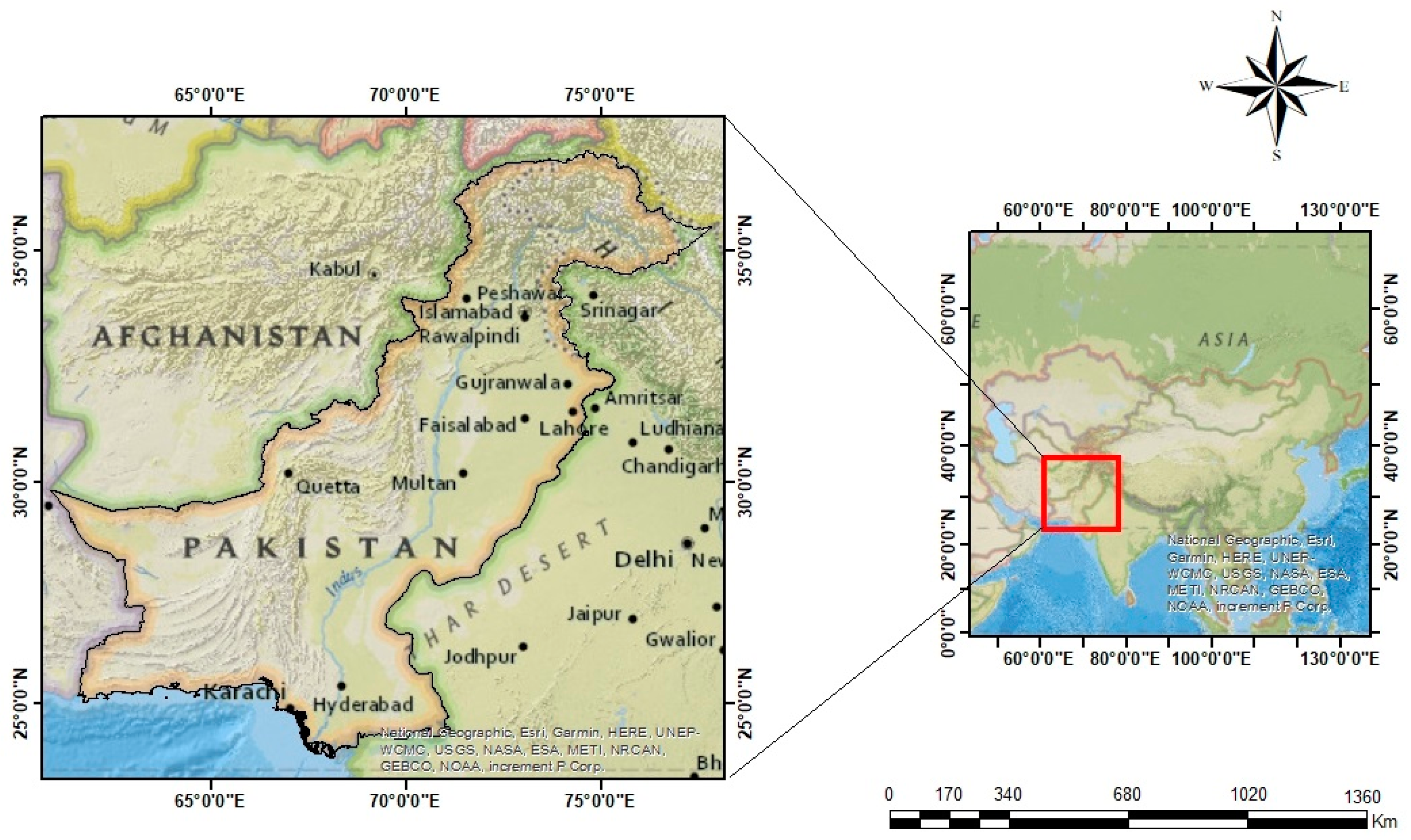
2.1. Study Area

The study area is the southwest Asian country named Pakistan (Figure 1), which is located at 30.3753° North latitude and 69.3451° East longitude. It connects the Hindukush Mountains on the north side and extends from the Pamirs to the Arabian Sea on the south side. Pakistan is divided into four provinces: Punjab, Sindh, Khyber Pakhtunkhwa (KPK), and Baluchistan. Pakistan’s climate ranges from arid to humid subtropical, with five distinct seasons: winter, spring, monsoon, summer, and autumn [29]. The month of June is the hottest, with a mean daily temperature exceeding 38 °C [30]. In comparison to June, July is the wettest month, with thunderstorms, the possibility of flooding, and cloudbursts. January, on the other hand, is the most refreshing month of the year [31]. The monsoon season begins at the end of May. However, the weather is behaving unpredictably when compared to previous years. Khan, in his study [32], elaborated that the precipitation patterns in Pakistan have become severely uncertain and heavy for shorter timespans. Extreme weather conditions such as extreme temperature, erratic rainfall, and climate-related shocks (floods, dust cyclones, and drought) have significantly influenced Pakistan [33]. The average global temperature has risen by approximately 0.6–0.8 °C in the last decade and is expected to continue rising at a rapid rate [34]. Globally, Pakistan is the seventh most affected country by climate change [35]. Extreme weather-related risks cost the country about PKR 365 billion annually because of inadequate water supply, deforestation, pollution, and soil degradation [36].

2.2. Datasets Used in the Study

COVID-19 cases, climatic factors, and environmental pollutants were used in this study. We used total COVID-19 cases, daily new cases, and total deaths between February 2020 and February 2021 to create a pandemic overview. For climatic factors, daily temperature (maximum, minimum, and mean) (°C), daily precipitation (mm), and daily wind speed (m/s) have been used. The environmental pollutants data are taken from satellite observation and described in

Table 2. Detail description of the datasets used in the present study.

Level of Study	Datasets	Spatial Resolution	Temporal Resolution	Acquisition Date	Sensor/Provider	Data Sources
Country Level	Tropospheric NO2	0.25°	Daily	2020–2021 (January–February)	Ozone monitoring instrument (OMI)	https://giovanni.gsfc.nasa.gov/giovanni/ (accessed on 30 May 2020)
	Dust Column Mass Density PM2.5	0.5 × 0.625°	Hourly	2020–2021 (January–February)	MERRA-2 Model	https://giovanni.gsfc.nasa.gov/giovanni/ (accessed on 30 May 2020)
	Total Column O3	1°	Daily	2020–2021 (January–February)	Ozone monitoring instrument (OMI)	https://giovanni.gsfc.nasa.gov/giovanni/ (accessed on 30 May 2020)
	Urban mobility value	Average over country	Daily	2020–2021 (February–February)	Our world in data (Google reports)	https://ourworldindata.org/ (assessed on 10 March 2020)
	COVID-19 data	Average over country	Daily	2020–2021 (February–February)	Our world in data (Google reports)	https://ourworldindata.org/ (assessed on 10 March 2020)
	Climate data	Average over country	Daily	2020–2021 (February–February)	NASA Prediction of Worldwide Energy Resources (POWER)	https://power.larc.nasa.gov/data-access-viewer/ (assessed on 15 April 2020)
City Level	NO2	0.1°	Monthly	2016–2020 (January–December)	Ozone monitoring instrument (OMI)	https://mynasadata.larc.nasa.gov/ (assessed on 20 December 2020)
	Ozone	0.25°	Monthly	2016–2020 (January–December)	Ozone monitoring instrument (OMI)	https://mynasadata.larc.nasa.gov/ (assessed on 20 December 2020)
	SO2	0.1°	Monthly	2016–2020 (January–December)	Ozone monitoring instrument (OMI)	https://mynasadata.larc.nasa.gov/ (assessed on 20 December 2020)
	Aerosol Optical Depth (AOD)	0.5°	Monthly	2016–2020 (January–August)	Visible Infrared Imaging Radiometer Suite (VIIRS)	https://mynasadata.larc.nasa.gov/ (assessed on 20 December 2020)

.

2.3. Data Analysis

The NASA Giovanni user interface was used to process daily data of tropospheric NO₂, O₃, and hourly PM_2.5. As previously stated, the Pakistani government declared a strict lockdown on 1 April 2020. The analytical scheme is divided into three discrete periods to evaluate the effects of COVID-19: (1) Before lockdown (January–March 2020), (2) Strict lockdown (April–June 2020), and (3) Loosening lockdown (June 2020) (July 2020–February 2021). Time series maps of various quarantine scenarios were created using the acquired datasets from January 2020 to February 2021. Furthermore, we used the vigorous data analysis pattern described below to identify changes and detect the relationship between the variables.

2.3.1. Anomaly Changes

The NASA Earth System Data Explorer was used to refine monthly NO₂, SO₂, O₃, and AOD data. It is a web application that provides a suitable and user-friendly interface for visualizing, analyzing, and accessing remote sensing data. This study computed daily anomaly changes using absolute difference.

2.3.2. Pearson Correlation

Pearson correlation has been used to analyze the three types of datasets. We used a Pearson correlation coefficient test to determine the relationship between the datasets. The p-value indicated the statistical significance of the association, and the Pearson coefficient represented the change in the variables, which could be positive or negative. The Pearson coefficient is calculated as follows:

$$\rho =\frac{ \Sigma (\mathrm{G} - \hat{\mathrm{G}})(\mathrm{H} - \hat{\mathrm{H}})}{ \sqrt{{\Sigma (\mathrm{G} - \hat{\mathrm{G}})}^2 {\Sigma (\mathrm{H} - \hat{\mathrm{H}})}^2}}$$

(1)

If $\rho$ is +1, it indicates a highly positive relationship between the variables. If $\rho$ is −1, it shows a highly antagonistic relationship. A zero value indicates that there is no relationship between variables. The results are presented in

Table 3. Results of Pearson correlation (ρ) with Urban mobility and Air pollutants.

Parameters	R&R	G&P	Parks	TS	Workplaces	Residential	NO2	SO2	O3
R&R	1.000 *
G&P	0.954 *	1.000 *
Parks	0.978 *	0.931 *	1.000 *
TS	0.982 *	0.985 *	0.951 *	1.000 *
Workplaces	0.972 *	0.907 *	0.916 *	0.951 *	1.000 *
Residential	−0.981 *	−0.899 *	−0.958 *	−0.937 *	−0.970 *	1.000 *
NO2	−0.438	−0.467	−0.313	−0.502	0.130	0.181	1.000 *
SO2	0.225	0.486	0.347	0.482	0.366	−0.223	−0.205	1.000 *
O3	−0.491	−0.636 *	−0.576 *	−0.538	−0.374	0.417	−0.229	−0.383	1.000 *

G&P = grocery and pharmacy, TS = transit stations, R&R = retailer and recreational places. * Level of significance = 0.05.

and

Table 4. Pearson Correlation association between air pollutants and climatic parameters.

Parameters	NO2	SO2	O3	AOD	Tmax	Tmean	Tmin	Precipitation	Wind Speed
NO2	1.000 *
SO2	−0.205	1.000 *
O3	−0.229	−0.383	1.000 *
AOD	0.698	0.582	−0.889 *	1.000 *
Tmax	0.899 *	−0.445	−0.218	0.579 *	1.000 *
Tmean	0.900 *	−0.462	−0.103	0.691 *	0.985 *	1.000 *
Tmin	0.879 *	−0.465	−0.001	0.771 *	0.949 *	0.989 *	1.000 *
Precipitation	0.005	−0.394	0.588 *	0.375	0.03	0.123	0.199	1.000 *
Wind Speed	−0.301	0.524	−0.048	−0.498	−0.412	−0.477	−0.521	−0.216	1.000 *

* Significance level = 0.05.

.

2.3.3. Kruskal–Wallis H Test (KWt) and Wilcoxon Signed Rank Sum Test (WRST)

We strongly believe that there was a significant increase/decrease in the mobility indices during strict lockdown and loosening lockdown. To check the impact of certain lockdown time on mobility indices, we considered KWt. It is a famous nonparametric test for comparing the outcomes between more than two independent groups. This test is used to compare mean ranks of k groups (k > 2) and is sometimes illustrated as an ANOVA with their ranks. For the massive literature about KWt, see [37,38,39].

In the case of a significant difference between the mean ranks of the different lockdown groups, we used WRST for pairwise comparison among mobility trend before lockdown (BL), during strict lockdown (SL), and during loosening lockdown (LL). WRST is a popular nonparametric test and is used widely in engineering, environmental, and medical etc. [40,41]. For all analyses, (p < 0.05) is considered significant and the results are shown in

Table 5. Kruskal–Wallis test and Wilcoxon statistics for Pakistan in the period of February 2020–January 2021.

Parameter	BL	SL	LL	Kruskal Wallis Test	p-Value
	Mean Rank	Mean Rank	Mean Rank
R&R	247.49 a	76.01 b	208.32 c	127.299	0.001 *
G&P	167.27 a	61.52 b	229.66 c	171.087	0.001 *
Parks	174.39 a	58.30 b	229.97 c	177.974	0.001 *
TS	190.32 a	67.52 b	223.06 c	146.550	0.001 *
Workplaces	268.77 a	87.51 b	199.43 c	112.922	0.001 *
Residential	107.93 a	259.97 b	160.78 c	83.370	0.001 *

Fixed at the * significance level = 0.05. Different lower case super scripts row wise shows the significant (p < 0.05) difference among lockdown groups by using the Wilcoxon rank-sum test.

.

2.3.4. Percentage Reduction

The percentage reduction approach is also being used in this study to determine how much of the air pollutants have been influenced by the COVID-19 lockdown. The monthly data of air pollutants in 2020 was compared to the same month of the baseline period (mean 2016–2019) to determine how much the data in 2020 increased or decreased in comparison to the baseline, just as the study of Zhang et al. [4] (

Table 6. Percentage changes in NO₂, O₃, and AOD concentrations when comparing the 2020 lockdown period to the same period in 2016–2019 across the three metropolitan cities of Pakistan. (Note: AOD data is only available until August 2020).

City	Month	NO2	O3	AOD	Status
		%	%	%
Lahore	January–March	12.09	6.57	−9.11	BL
	April–June	−0.14	0.23	−14.46	SL
	July–December	11.55	−0.38	−7.96	LL
Islamabad	January–March	−4.39	6.16	20.44	BL
	April–June	−11.21	0.55	−22.65	SL
	July–December	16.14	−0.55	−14.98	LL
Karachi	January–March	−14.06	6.31	−7.66	BL
	April–June	−27.87	0.67	−13.70	SL
	July–December	0.02	0.53	−20.88	LL

).

2.3.5. Generalized Linear Models (GLM)

To be more precise, to investigate the relationship of COVID-19 cases with climatic parameters and air pollutants, we used the GLM (Mehmood et al. [26]) (

Table 7. Generalized Linear Model (GLM) parameters estimates for Pakistan in the period of Feb 2019–Jan 2020.

Parameter	B	Std. Error	95% Wald Confidence Interval		Df	p-Value
			Lower	Upper
(Intercept)	0
Tmax	1706.874	449.482	717.571	2696.176	1.000	0.004 *
Tmean	2297.072	647.926	870.996	3723.149	1.000	0.005 *
Tmin	3078.853	1024.806	823.271	5334.435	1.000	0.013 *
Precipitation	174.018	99.014	−43.911	391.947	1.000	0.109
Wind Speed	14,676.698	3816.019	6277.697	23,075.698	1.000	0.003 *
NO2	54,285.023	12,092.254	27,670.152	80,899.894	1.000	0.001 *
SO2	424,675.359	149,860.398	94,834.848	754,515.871	1.000	0.018 *
O3	128.670	35.046	51.534	205.806	1.000	0.004 *

Dependent Variable: COVID-19 Cases; Model: (Intercept): Covariates: Air pollutants. Temperature, Precipitation, Wind speed. Fixed at the * significance value p < 0.05.

). The GLM is a flexible technique with the ordinary least square regression estimation, which allows for different variables that have error distributions other than a normal distribution. The characteristics of the GLM model is that, we can estimate the parameters of the models with the link function. This link function helps us to understand how strong the variance is for each observation to forecast value. Equations (2) and (3) shows the standard GLM mathematical expression, whereas the link and mean equation is estimated through Equations (4) and (5):

$$y_i|b~Dist\left( {\mu }_i, \left(\frac{{\sigma }^2}{w_i}\right)\right)$$

(2)

$$g\left(\mu \right)=X\beta +Zb+\delta$$

(3)

$$X\beta =\ln \left(\mu \right)$$

(4)

$$\mu =\exp \left(X\beta \right)$$

(5)

where $y_i$ represent the ith element of the response variable vector, whereas $b$ is the random effect vector. Dist is a conditional distribution of the response variable $y_i$ given by $b$. $\mu$ shows the conditional mean of $y$ given $b$, where$i$ always represent the ith element of the any mentioned variable. ${\sigma }^2$ depicts the dispersion parameter, and $w_i$ represents observational weight vector. In this study, COVID-19 cases are considered as the dependent variable, whereas ${\mathrm{NO}}_2,{ \mathrm{SO}}_2$, ${\mathrm{O}}_3$, and climatic parameters are considered as covariates. The Poisson distribution and log link function estimate the parameters. We ran the analysis by using the R software version 3.3.2, and the “MASS” package is further used to obtain the estimates of the parameter of GLM.

3. Results and Discussion

Satellite observation of climate and air pollution datasets, COVID-19, and mobility datasets are analyzed in this study to show how changes in air pollutants from a spatiotemporal proportion caused a change in climate parameters in response to COVID-19 quarantine measures. Variations in air pollution result in changes in climatic parameters.

The air pollutants (NO₂, SO₂, O₃) are correlated with the climate data to assess their relationship. The findings revealed that temperature and precipitation are positively correlated with tropospheric NO₂ concentrations, in contrast to previous studies that showed mixed results, indicating that temperature was either a positive [42,43] or negative [44] facet for NO₂. Precipitation is usually the cause of NO₂ reduction through washout. Many studies have discovered a negative relationship between precipitation and NO₂ [44,45], but similar to Harkey et al. [46], our study also depicted a positive correlation between precipitation and tropospheric NO₂. The reduction in NO₂ due to precipitation might be exacerbated by an increase in wind speed, so they have a negative association between them having Pearson coefficient value ρ = −0.301 (Table 4). Similarly, temperature and precipitation are negatively correlated with SO₂ concentration, but wind speed is positively correlated (ρ = 0.524).

We used three Pakistani metropolitan areas (Islamabad, Lahore, and Karachi) to visualize the timeseries data influenced by the lockdown. As a baseline period, the monthly mean air pollutants data (NO₂, SO₂, O₃, AOD) from January 2016 to December 2019 was considered. This average data was compared to the data obtained in 2020. Following that, for a city-level analysis, the mean time series data from satellite observations for three metropolitan areas were used to investigate air pollution variations in response to the COVID-19 quarantine. From February to March 2020, the area was distinguished by regular late-winter variability and evidence of spring’s arrival. The period also shows the fluctuation of wind patterns and the intensity and direction of flow. To determine whether meteorological conditions existed during the examined period, a brief analysis was performed by comparing time series data of surface factors affecting the ground atmosphere at current times [47].

3.1. COVID-19 and Lockdown Setups in Pakistan

There were only four cases reported in Pakistan as of 1 March 2020 [48]. However, because of the movement of people to and from other parts of the world, particularly from China and Iran via the Taftan Border, the number of cases suddenly increased. Furthermore, the first quarantine was announced only in Sindh province on 23 March 2020. It was later implemented in other parts of the country as well [30,49]. Protocols were enforced to prevent the spread of the virus, including the use of masks and sanitizers, social distancing, and so on. Nonetheless, migrants were returning to their hometowns, making the lockdown situation impossible. As a result, from mid-March 2020 to mid-April 2020, the cases ranged from 53 to 1078. On 18 October 2020, there were 323,019 cases and 6654 deaths reported in Pakistan [50]. To follow that, the number of cases is increasing dramatically in various parts of the country daily. Figure 2a depicts the new cases data obtained from a Google search. Figure 2b depicts the total cases documented by the WHO up to 8 February 2021: 556,519 total cases, 1008 new cases, and 12,066 total deaths. Given the current situation, the government of Pakistan has declared an SL beginning in April 2020 and lasting until June 2020. Following that, an LL was carried out in accordance with the number of cases [51].

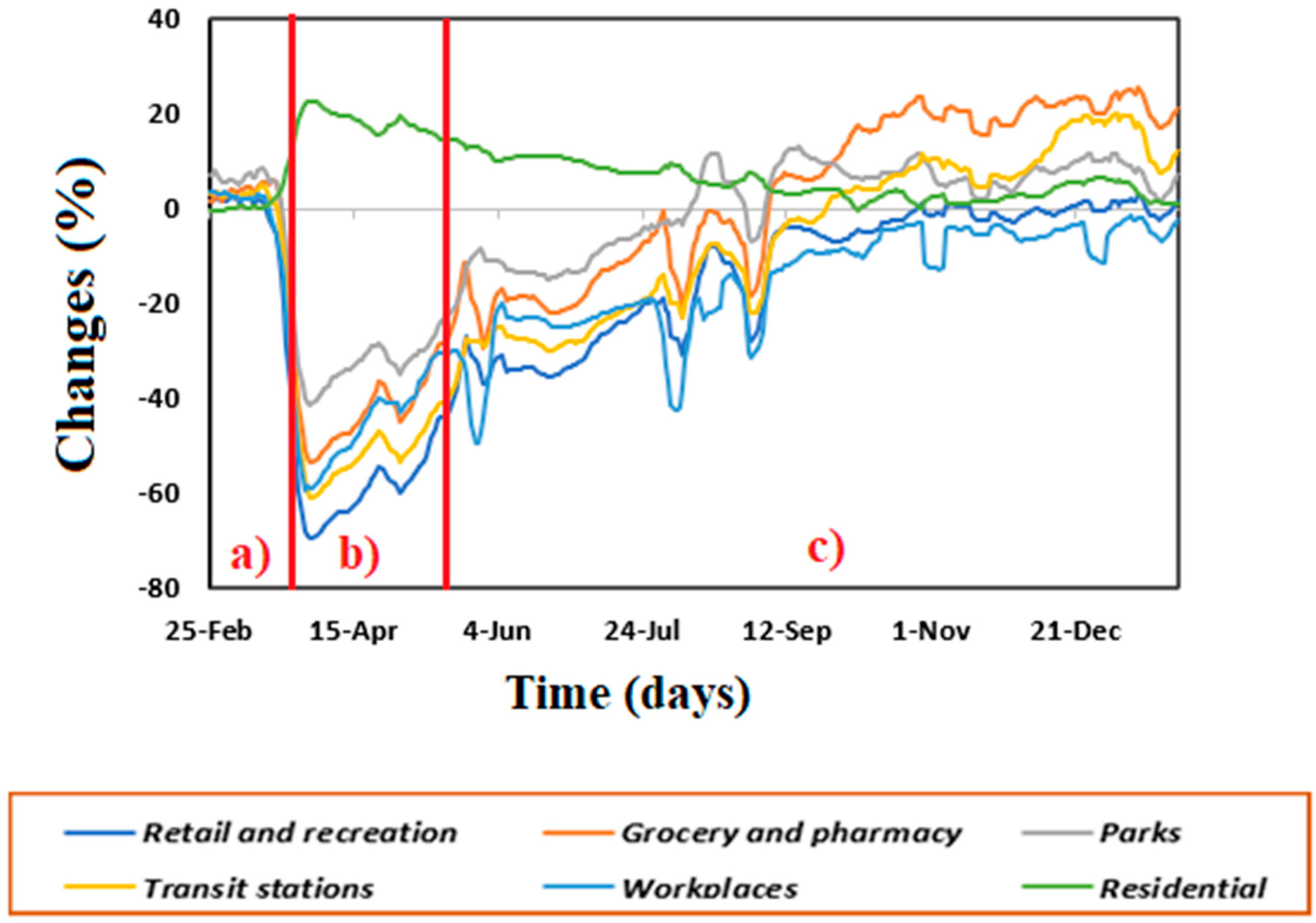
3.2. COVID-19 and Urban Mobility

The COVID-19 pandemic has impacted the pattern of human mobility [41,52]. The approach of substantial constraint has a significant influence on the pattern of demographic change in economies, groceries and pharmacies, and parks [53]. Nonetheless, the impact of lockdown and restricting activities has a positive influence on our environment, such as noise reduction, pollution, and improvement in air quality [54,55]. Many reports elaborated on how mobility patterns in most countries worldwide have decreased in response to an immediate halt to anthropogenic activities due to quarantine protocols [56,57,58]. Because of these circumstances, mobility patterns have suffered a severe breakdown.

This study examines the impact of pandemic quarantine stages on human actions using timeseries data. Figure 3 illustrates the variations in the mobility of anthropogenic actions over time in Pakistan. The trends in Google mobility reports classified normal mobility movements and actions as follows: parks, retail; and recreation; workplaces, grocery and pharmacy; transit stations; and residential. It is undeniable that all operations, such as transportation, educational institutions, workplaces, industries, and social sites, were operating normally before quarantine, but after quarantine was imposed, the urban mobility index dropped dramatically. Similarly, to the study of Shafeeque et al. [59], our results evidence that the urban mobility trend was reduced by 60–70% in Pakistan during quarantine. An apparent reduction in public activities of up to 80% as a result of quarantine enforcement has been observed in Figure 3, but it started to increase again in the LL period.

On the contrary, the mobility index of residential areas has increased since the quarantine began. As the pandemic began, Pakistan’s mobility index has decreased by 70–90% in workplaces and 60–85% in transit stations through 25 May 2020 [60]. In Pakistan, all activities, including public transportation and workplaces, were running on a trial basis until March 2020, when the government announced an SL [27].

The Google data show a decrease in human mobility patterns and an increase in the amount of time spent on a daily basis in residential areas [61]. It is obvious that as the cases increased, the movement of people was restricted. Therefore, the use of transportation was reduced enormously. Industries and other workplaces were also not in working conditions, which resulted in less fossil fuel consumption. Resultantly, we performed a Pearson correlation between urban mobility and air pollutants, and the results are presented in Table 3.

Table 5 represents the KWt and WRST results. The data has been divided into three groups: BF, SL, and LL. At the first step, KWt implies that there is a significant (p < 0.05) difference between the mean ranks of all three groups of R&R. The results show that mean rank of the SL is significantly lower than the BL and LL. The same pattern is observed for the G&P, where all the lockdown groups are significantly (p < 0.05) different from each other. SL has much lower and more significant (p < 0.05) mean rank values from other two lockdown groups. It is observed in Table 5 that the mean ranks of the Parks, TS, Workplaces, and Residential areas are significantly (p < 0.05) different from each other at different times of lockdown. After the significant results, the WRST is applied to check the pairwise comparison of the mean ranks of all parameters at different times of lockdown. The WRST illustrated that there is a significant (p < 0.05) difference among the mean ranks of BL and SL, BL and LL, and SL and LL.

The results clearly show that urban mobility has significantly reduced during the SL of all the parameters except in the residential area, where it has increased compared to BL [52,59]. It is also evident that the mobility has started to rise in the LL compared to the SL because all the activities started in that period, but it is less than BL.

3.3. COVID-19 Lockdown Impacts on the Eco-Environment

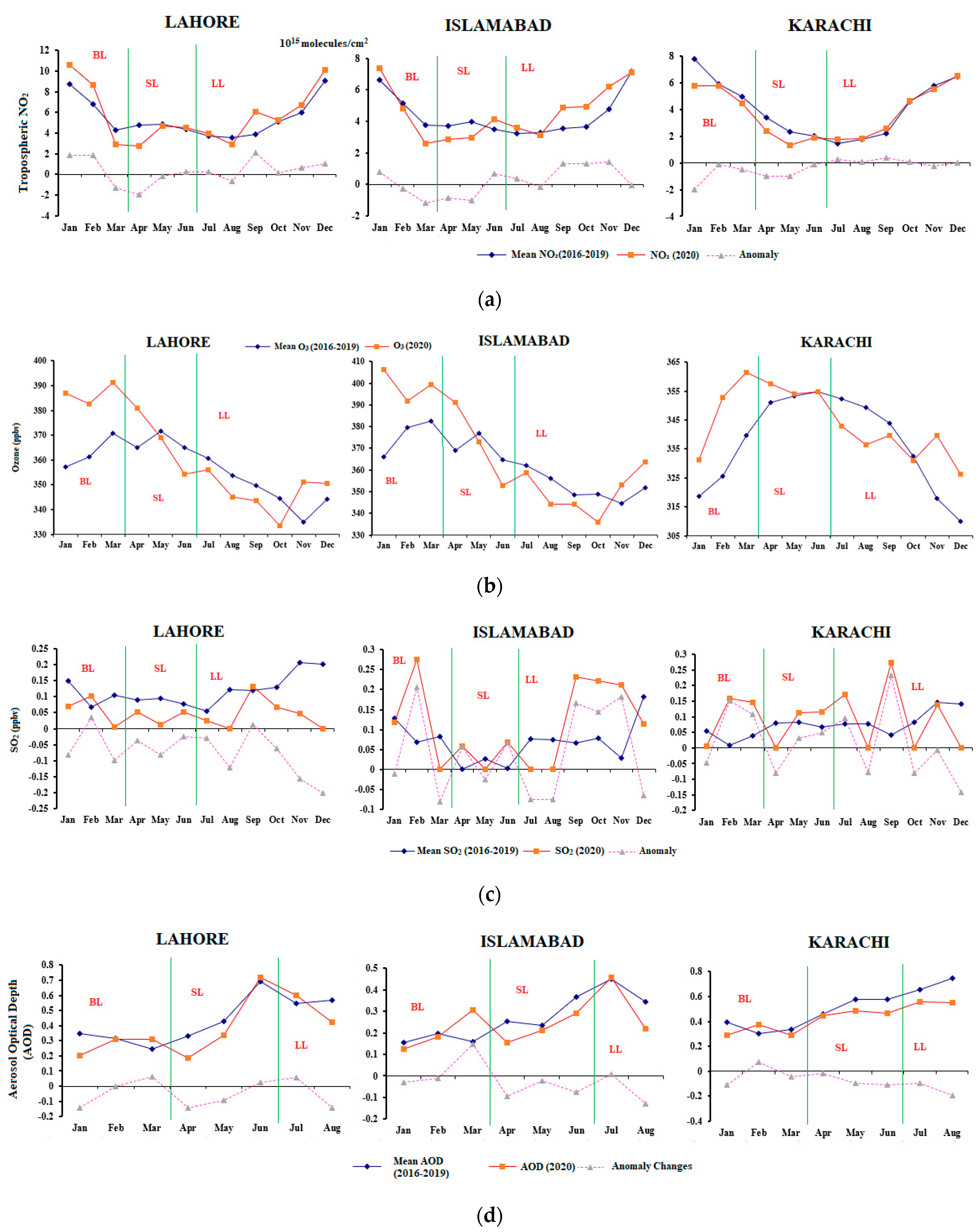
3.3.1. COVID-19 Lockdown Impact on Atmospheric Pollution

Due to the extreme pandemic, air quality has become the primary focus of atmospheric research. The study considers several changes in air pollutant concentrations because of reduced human activity [62,63,64]. The spatial and temporal variations are subsequent to the lockdown’s impact on air quality. The effects of air pollution on life are complicated. In addition to pollution source emissions, climatological conditions also have an effect on air quality [65]. In this study, we used satellite observations of various types of air pollutants, as shown in Table 2.

(a)

NO₂

Figure S1 demonstrates the variations in tropospheric column NO₂ concentrations. It manifests the daily time-averaged data of BL (January–March 2020), SL (April–June 2020), and LL (July 2020–February 2021). The maps of tropospheric NO₂ concentrations revealed that the high level of NO₂ emissions appeared before the lockdown due to mobility conditions, and the NO₂ concentrations rise across Pakistan from north to south, emerging from urban activities, transportation, and the industrial sector in Rawalpindi-Islamabad, Lahore, and Peshawar in the north to Karachi in the south (Figure S1). In the study of Zheng et al. [66], the concentration of NO₂ decreases as the temperature rises (see Figure S4 for temperature behavior (T_max, T_min, and T_mean)). Notwithstanding, before the lockdown, the spatiotemporal patterns of the tropospheric NO₂ concentration over Pakistan showed a relatively smooth pattern [67]. However, during the pandemic lockdown period in 2020, a decrease in NO₂ concentration was discovered. Compared to other provinces, Punjab is rich in NO₂ production due to urbanization, heavy traffic, and industrialization [59,68]. The European Union Copernicus Program, via the Copernicus Sentinel-5P satellite, released some new satellite images, claiming that NO₂ emissions were down ~40–50% in March–April 2020 compared to the same time period over Pakistan [69]. The current improvement in air quality is due to less fossil fuel combustion during the country’s imposed lockdown measures [69,70]. According to NASA’s Air Quality Space Observation Laboratory, the generation of energy around Pakistan has decreased by 10–25% during the quarantine period [71]. Additionally, this study examined the temporal variations in NO₂ emissions in BL, SL, and LL, particularly in three Pakistani metropolitan cities (Lahore, Islamabad, and Karachi) (Figure 4).

(b)

Ozone

Ozone (O₃) is a gas that occurs naturally at both the ground and the upper levels of the Earth’s atmosphere (stratosphere) [72]. Nevertheless, stratospheric ozone is considered “good” because it acts as a barrier to ultraviolet rays heading towards Earth. At the same time, the same O₃ in the troposphere and at ground level is a secondary air pollutant produced by a variety of actions, including urbanization and industrialization. Although ozone cleans the environment, it is also a significant greenhouse gas that is increasing due anthropogenic activities and energy production, contributing to climate change [72]. The overall change in ozone concentration has been depicted after the SL was implemented. Figure S2 represents a change in ozone during the SL versus before the lockdown was imposed. However, when we compared total column ozone before and after the SL, we could easily see a significant reduction in ozone concentration. This change has only occurred as a result of the cessation of public transportation.

(c)

PM_2.5

PM_2.5 is hazardous to both the environment and to human health [73,74,75]. Particulate matter has high environmental value, but it is also a significant contributor to air pollution, contributing to climate variability. PM_2.5 is emitted from various sources in Pakistan, with approximately 60% emitted from households, such as wood-burning during the winter, vehicle smoke, and non-exhaust transportation emissions throughout the year [76,77]. At the same time, the remainder is attributable to industries. PM_2.5 concentrations, similar to NO₂ concentrations, were at their lowest during the SL period compared to previous years [78]. Figure S3 symbolizes an obvious fluctuation in the spatial extent and magnitude of PM_2.5. Compared to before quarantine, the concentration of PM_2.5 dropped dramatically during the quarantine period (April–June).

(d)

City Level Analysis

The SL period (March–June 2020) during the COVID-19 Pandemic caused a decrease in energy consumption, power generation, and oil demand, which benefited our planet [79]. Figure 4a–d demonstrates the variation in air pollutants during 2020 compared to the baseline period (2016–2019) in Pakistan’s three major cities: Lahore, Islamabad, and Karachi. These three cities are developed cities in Pakistan with international airports. A large number of people came from other countries, primarily China and Iran, which became the cause of the COVID-19 spread [80]. During the SL period (April–June), all three cities show a gradual reduction in NO₂, Ozone, SO₂, and Aerosol Optical Depth (AOD). Furthermore, when compared to other cities, Karachi showed an exceptional reduction in NO₂ emissions. April 2020 was observed to be the month with the most considerable decrease in NO₂ concentration, with a steady recovery to the previous scenario until the end of July [81]. A remarkable change in NO₂ levels was observed in Lahore due to major contributions from transportation, as transportation is thought to be a major contributor to nitrogen oxide (NO_x) emissions in Pakistan [82].

It has been discovered that the running mean of NO₂ value during January–March 2020 (BL) has a fluctuation trend that differs from the average time series of 2016 to 2019. During the SL period (April–June 2020), the time series of average NO₂ emissions over all three cities in Pakistan moves with a slight fluctuation when compared to the baseline period (2016–2019) [28]. It has been observed that for the cities of Lahore and Islamabad, the anomaly changes in NO₂ emissions from January to March 2020 (before the lockdown) show a positive trend, demonstrating the high emissions from industrial sources and transportation compared to previous years. Despite this, anomaly changes in NO₂ emissions from April to June 2020 (SL) show a negative trend due to industrial and transportation emissions reductions.

For NO₂ emissions (10¹⁵ molecules/cm²), the orange line represents the year 2020 values compared to the blue line, which shows the average baseline period of 2016 to 2019. The vertical green line divides the quarantine period into three phases. According to the newly formed reports of NASA (National Aeronautics and Space Administration) and the ESA (European Space Agency) and other research in their studies, air pollution has eloquently decreased across metropolitan and industrialized areas over the last few months [69,71,83] because of the strict quarantine measures implemented by the government [84]. As per the results (Table 6), a consequential reduction of about 0.14% in NO₂ concentration has been observed in Lahore, 12% in Islamabad, and 28% in Karachi. Though exceptions are there, it again started increasing to the previous value in December 2020.

Figure S2 and Figure 4b display the spatial and temporal variations in O₃ concentration for Pakistan and the city-wise distribution. It has established a gradual decrease during SL (April–June 2020) and the beginning of an LL in July 2020. Compared to the baseline period, a major reduction in O₃ has not been found during the SL. However, after June in the LL period, a slight reduction was evident in the cities of Pakistan presented in Table 6. Nonetheless, a significant increase in O₃ was observed in Pakistan between March and April 2020 in the study of [4].

Both natural and anthropogenic processes cause SO₂ establishment. It occurs naturally as a result of volcanic eruptions, and man-made sources include fuel combustion, energy generation, and metal fusion [85]. Its presence in the lower troposphere layer can reduce air quality, and it is also a precursor originator of gases, including sulfate aerosols, which influence cloud reflectiveness. If hydrogen peroxide (H₂O₂) is available in the atmosphere along with the presence of O₃, it can predominantly oxidize the molecules of SO₂ and eventually produce sulfuric acid (H₂SO₄), which can further produce sulfate. Furthermore, sulfates are the mainstay of particulate matter (PM_2.5) and account for 11–65% of aerosol mass [20]. Figure 4c manifests a temporal variation in SO₂ concentration in 2020 compared with the baseline period of 2016–2019. The results show a significant reduction in SO₂ concentration through anomaly changes as ~53% in Lahore, ~38% in Islamabad, and ~45% in Karachi.

Per annum, aerosol particles are released due to anthropogenic activities which give rise to the hazardous levels of air pollution over the major cities such as Lahore, Islamabad and Karachi in Pakistan [86,87]. The atmosphere can be considered clean if the value of AOD is less than 0.1 over the whole atmospheric vertical column. However, the greater values of AOD, even 1 or higher, designate a very hazy situation and that the air is polluted. Figure 4d presented the datasets released by NASA, showing a decline in AOD in the year 2020, particularly in April to mid-May compared to the baseline period (2016–2019). As the datasets are only available until Aug 2020, we have used the monthly mean AOD data for the years 2016–2019 from January–August as a baseline period for a well-defined comparison. The reduction in AOD is in accordance with the pandemic quarantine on account of the lower emission of particles (such as NO_X, SO_X). However, an immense reduction in AOD, such as 14% in Lahore, 23% in Islamabad, and 14% in Karachi, has been observed.

3.3.2. COVID-19 Lockdown and Climatic Parameters

As discussed in the previous section, the lockdown situation in Pakistan reduces air pollutants and greenhouse gas (GHG) emissions, which ultimately leads to variations in climatic parameters [88]. Both COVID-19 and weather patterns are global issues with extraordinary and highly uncertain consequences [89,90]. Aside from changes in urban mobility, climatic factors have been impacted by the COVID-19 pandemic because of reduced transportation use. In Table 4, the climatic parameters are correlated with air pollutants to find out the change. The results revealed that temperature and precipitation are positively correlated with NO₂ and AOD, but wind speed is negatively correlated. Temperature also showed a significant (p < 0.05) change with NO₂ and AOD. Opposite to the wind speed, temperature and precipitation showed a negative association with SO₂. However, temperature and wind speed depicted a negative association with O₃, and precipitation showed a positive and significant (p < 0.05) association. We have performed a GLM between COVID-19 and air pollution and climatic parameters. The results in Table 7 illustrate that all the air pollutants and climatic parameters show a significant (p < 0.05) change, except precipitation.

Figure S4 illustrates a series distribution of COVID-19 cases and climatic parameters (Temperature, Precipitation, and Windspeed) along with the lockdown status in Pakistan. The curve of daily COVID-19 cases has reached a peak during June, which has a good trend with wind speed and precipitation. It is possible to see how precipitation abruptly decreased in SL situations. When the wind intensity is considered, comparable patterns of flow reduction can be detected for Pakistan’s SL and LL periods.

Other than that, T_max, T_min, and T_mean have the opposite direction to the COVID-19 cases data. It does not exhibit more critical fluctuations, although it is a crucial factor while discussing the influence of COVID-19. The relationship between temperature and COVID-19 cases offers valuable information in terms of its prevalence across Pakistan. It has been observed that COVID-19 cases have a lesser influence on temperature (T_max, T_min, and T_mean). Through Figure S4, it can be clearly observed that the values of temperature (T_max, T_min, and T_mean) were higher during the BL period, and as COVID-19 began, it had an abrupt decline. However, during the SL, when COVID-19 cases were at their peak, the temperature (T_max, T_min, and T_mean) also showed a sudden rise (35%) due to an average 40% reduction in tropospheric NO₂ concentration during the SL period [66].

4. Conclusions

The SL measures implemented across Pakistan not only halted the spread of the COVID-19 virus but also had a positive impact on the environment. The study’s hypothesis was that by restricting human movement, goods-trafficking, and social and industrial activities, the air pollution has been reduced significantly. Because of that, changes in air pollution caused by a ~20–30% reduction in NO₂ emissions have also predisposed the weather to change positively. The findings of this study show that since April 2020, there has been a consequential decrease (~20–30%) in air pollution in Pakistan, such as Karachi seeing a 28% decrease in NO₂ concentrations, and a 23% decrease in AOD in Islamabad during the SL. In contrast, a minor 0.55% decrease in O₃ is evident in Islamabad during the LL.

Furthermore, the regression model investigated a significant (p < 0.05) reduction in SO₂, O₃, and NO₂ emissions and climatic parameters except precipitation due to the less reliance on fossil fuels, which justified our reduction analysis results. The results of the KWt and the WRST revealed that the mean rank of the SL is significantly lower than the BL and LL only because of restrictions on human movement.

According to the findings of this study, some strategies have been recommended to improve urban air quality management, which include:

○

The government of Pakistan should impose such stringent restrictions on the use of fossil fuels. Similar to China, they should promote short individual trips on foot or by switching vehicles (e.g., motorbikes and Qingqi) to bicycles and scooters.

○

Catalytic converters are required in all large vehicles.

○

The personal mode of transportation must be replaced by group travel or local buses.

○

Controlling the emissions from large point sources.

○

The conversion of diesel-fueled buses and vans to CNG and the installation of diesel oxidation catalysts in metro and other big city buses.

○

The local government should impose some brief lockdowns (1–2 days) once a month on fossil fuel consumption and human transportation, particularly in Lahore, which has experienced the deadliest smog in the last five years.

In response to the results of the KWt and the WRST, the authors have suggested that policymakers follow the Sustainable Urban Mobility Plan (SUMP) approach for urban mobility planning, which is a strategy document meant to fulfill the demand for mobility while also maintaining an appropriate quality of life for inhabitants. This technique can also assist in mitigating the harmful effects of urban transportation. The SUMP process can be aided by a transport model known as the Multilevel Model of Transport Systems (MST). The involvement of citizens and stakeholders should be included throughout the planning process. The article proposed using the MST at various levels of planning and modelling and describing the consequences. The use of a hierarchical layout will assist in fully realizing the transport model’s potential to increase the efficacy of urban mobility planning.

References

1. Wang, L.; Wang, Y.; Ye, D.; Liu, Q. Review of the 2019 novel coronavirus (SARS-CoV-2) based on current evidence. Int. J. Antimicrob. Agents 2020, 55, 105948. [Google Scholar] [CrossRef] [PubMed]
2. Zoran, M.A.; Savastru, R.S.; Savastru, D.M.; Tautan, M.N. Assessing the relationship between ground levels of ozone (O3) and nitrogen dioxide (NO2) with coronavirus (COVID-19) in Milan, Italy. Sci. Total Environ. 2020, 740, 140005. [Google Scholar] [CrossRef] [PubMed]
3. Morita, H.; Nakamura, S.; Hayashi, Y. Changes of urban activities and behaviors due to COVID-19 in Japan; SSRN: Rochester, NY, USA. Available online: https://papers.ssrn.com/sol3/papers.cfm?abstract_id=3594054 (accessed on 15 February 2020).
4. Zhang, Z.; Arshad, A.; Zhang, C.; Hussain, S.; Li, W. Unprecedented temporary reduction in global air pollution associated with COVID-19 forced confinement: A continental and city scale analysis. Remote Sens. 2020, 12, 2420. [Google Scholar] [CrossRef]
5. Dhar, S.; Shukla, P.R. Low carbon scenarios for transport in India: Co-benefits analysis. Energy Policy 2015, 81, 186–198. [Google Scholar] [CrossRef] [Green Version]
6. Krzyzanowski, M.; Kuna-Dibbert, B.; Schneider, J. Health Effects of Transport-Related Air Pollution; WHO Regional Office Europe: Geneva, Switzerland, 2005. [Google Scholar]
7. Fullerton, D.G.; Bruce, N.; Gordon, S.B. Indoor air pollution from biomass fuel smoke is a major health concern in the developing world. Trans. R. Soc. Trop. Med. Hyg. 2008, 102, 843–851. [Google Scholar] [CrossRef] [Green Version]
8. Gordon, S.B.; Bruce, N.G.; Grigg, J.; Hibberd, P.L.; Kurmi, O.P.; Lam, K.-B.H.; Mortimer, K.; Asante, K.P.; Balakrishnan, K.; Balmes, J. Respiratory risks from household air pollution in low and middle income countries. Lancet Respir. Med. 2014, 2, 823–860. [Google Scholar] [CrossRef] [Green Version]
9. Beig, G.; Sahu, S.K.; Singh, V.; Tikle, S.; Sobhana, S.B.; Gargeva, P.; Ramakrishna, K.; Rathod, A.; Murthy, B. Objective evaluation of stubble emission of North India and quantifying its impact on air quality of Delhi. Sci. Total Environ. 2020, 709, 136126. [Google Scholar] [CrossRef]
10. Conticini, E.; Frediani, B.; Caro, D. Can atmospheric pollution be considered a co-factor in extremely high level of SARS-CoV-2 lethality in Northern Italy? Environ. Pollut. 2020, 261, 114465. [Google Scholar] [CrossRef]
11. Maji, K.J. Substantial changes in PM2. 5 pollution and corresponding premature deaths across China during 2015–2019: A model prospective. Sci. Total Environ. 2020, 729, 138838. [Google Scholar] [CrossRef]
12. Rahman, M.; Rana, R.; Khanam, R. Determinants of Life Expectancy in Most Polluted Countries: Exploring the Effect of Environmental Degradation. Res. Sq. 2020, 1–27. Available online: https://assets.researchsquare.com/files/rs-77014/v1_stamped.pdf?c=1600797547 (accessed on 15 February 2020).
13. AirVisual, I.J.I.A. World Air Quality Report, Staad, Switzerland. 2018. Available online: https://www.airvisual.com/world-most-polluted-citie (accessed on 15 February 2020).
14. Ali, S.M.; Malik, F.; Anjum, M.S.; Siddiqui, G.F.; Anwar, M.N.; Lam, S.S.; Nizami, A.-S.; Khokhar, M.F. Exploring the linkage between PM2. 5 levels and COVID-19 spread and its implications for socio-economic circles. Environ. Res. 2021, 193, 110421. [Google Scholar] [CrossRef]
15. Raunak, R.; Sawant, N.; Sinha, S. Impact of Covid-19 on Urban Mobility in Indian Cities. Transp. Commun. Bull. Asia Pac. 2020, 90, 71–85. [Google Scholar]
16. Mehmood, K.; Saifullah, M.I.; Abrar, M.M. Can exposure to PM2. 5 particles increase the incidence of coronavirus disease 2019 (COVID-19)? Sci. Total Environ. 2020, 741, 140441. [Google Scholar] [CrossRef]
17. Shi, P.; Dong, Y.; Yan, H.; Zhao, C.; Li, X.; Liu, W.; He, M.; Tang, S.; Xi, S. Impact of temperature on the dynamics of the COVID-19 outbreak in China. Sci. Total Environ. 2020, 728, 138890. [Google Scholar] [CrossRef]
18. Hitchcock, G.; Conlan, B.; Kay, D.; Brannigan, C.; Newman, D. Air Quality and Road Transport. In Impacts Solutions; RAC Foundation: London, UK, 2014. [Google Scholar]
19. Cohen, A.J.; Brauer, M.; Burnett, R.; Anderson, H.R.; Frostad, J.; Estep, K.; Balakrishnan, K.; Brunekreef, B.; Dandona, L.; Dandona, R. Estimates and 25-year trends of the global burden of disease attributable to ambient air pollution: An analysis of data from the Global Burden of Diseases Study 2015. Lancet 2017, 389, 1907–1918. [Google Scholar] [CrossRef] [Green Version]
20. Seinfeld, J.H.; Pandis, S.N. Atmospheric Chemistry and Physics: From Air Pollution to Climate Change; John Wiley & Sons: Hoboken, NJ, USA, 2016. [Google Scholar]
21. WHO. Available online: https://apps.who.int/iris/bitstream/handle/10665/69477/WHO_SDE_PHE_OEH_06.02_eng.pdf (accessed on 18 June 2020).
22. Latha, R.; Murthy, B.; Sandeepan, B.; Bhanage, V.; Rathod, A.; Tiwari, A.; Beig, G.; Singh, S. Propagation of cloud base to higher levels during Covid-19-Lockdown. Sci. Total Environ. 2021, 759, 144299. [Google Scholar]
23. Kanga, S.; Meraj, G.; Farooq, M.; Nathawat, M.; Singh, S.K. Risk assessment to curb COVID-19 contagion: A preliminary study using remote sensing and GIS. Res. Square 2020, 1–19. [Google Scholar] [CrossRef]
24. Nakajima, K.; Takane, Y.; Kikegawa, Y.; Furuta, Y.; Takamatsu, H. Human behaviour change and its impact on urban climate: Restrictions with the G20 Osaka Summit and COVID-19 outbreak. Urban Clim. 2021, 35, 100728. [Google Scholar] [CrossRef]
25. Liu, J.; Zhou, J.; Yao, J.; Zhang, X.; Li, L.; Xu, X.; He, X.; Wang, B.; Fu, S.; Niu, T. Impact of meteorological factors on the COVID-19 transmission: A multi-city study in China. Sci. Total Environ. 2020, 726, 138513. [Google Scholar] [CrossRef] [PubMed]
26. Mehmood, K.; Bao, Y.; Abrar, M.M.; Petropoulos, G.P.; Soban, A.; Saud, S.; Khan, Z.A.; Khan, S.M.; Fahad, S. Spatiotemporal variability of COVID-19 Pandemic in relation to Air pollution, Climate and Socioeconomic Factors in Pakistan. Chemosphere 2021, 271, 129584. [Google Scholar] [CrossRef] [PubMed]
27. Ali, G.; Abbas, S.; Qamer, F.M.; Wong, M.S.; Rasul, G.; Irteza, S.M.; Shahzad, N. Environmental Impacts of Shifts in Energy, Emissions, and Urban Heat Island during the COVID-19 Lockdown Across Pakistan. J. Clean. Prod. 2021, 291, 125806. [Google Scholar] [CrossRef]
28. Arshad, A.; Hussain, S.; Saleem, F.; Shafeeque, M.; Khan, S.N.; Waqas, M.S. Unprecedented reduction in airborne aerosol particles and nitrogen dioxide level in response to COVID-19 pandemic lockdown over the Indo-Pak region. Earth Space Sci. Open Arch. 2020. [Google Scholar] [CrossRef]
29. Fowler, H.; Archer, D. Conflicting signals of climatic change in the Upper Indus Basin. J. Clim. 2006, 19, 4276–4293. [Google Scholar] [CrossRef] [Green Version]
30. Raza, A.; Khan, M.T.I.; Ali, Q.; Hussain, T.; Narjis, S. Association between meteorological indicators and COVID-19 pandemic in Pakistan. Environ. Sci. Pollut. Res. 2020, 28, 40378–40393. [Google Scholar] [CrossRef] [PubMed]
31. Ali, G. Climate change and associated spatial heterogeneity of Pakistan: Empirical evidence using multidisciplinary approach. Sci. Total Environ. 2018, 634, 95–108. [Google Scholar] [CrossRef] [PubMed]
32. Khan, M.A. Climate change risk and reduction approaches in Pakistan. In Disaster Risk Reduction Approaches in Pakistan; Springer: Berlin/Heidelberg, Germany, 2015; pp. 195–216. [Google Scholar]
33. Abid, M.; Schilling, J.; Scheffran, J.; Zulfiqar, F. Climate change vulnerability, adaptation and risk perceptions at farm level in Punjab, Pakistan. Sci. Total Environ. 2016, 547, 447–460. [Google Scholar] [CrossRef]
34. Bank, W. World Development Report 2012: Gender Equality and Development; The World Bank: Washington, DC, USA, 2011. [Google Scholar]
35. Kreft, S.; Eckstein, D.; Melchior, I. Who suffers most from extreme weather events? Global Clim. Risk Index 2017, 10, 1998–2017. [Google Scholar]
36. Economic Survey of Pakistan, Economic Advisor’s Wing; Ministry of Finance: Islamabad, Pakistan, 2018.
37. McKight, P.E.; Najab, J. Kruskal-wallis test. Corsini Encycl. Psychol. 2010, 1. [Google Scholar] [CrossRef]
38. Ostertagova, E.; Ostertag, O.; Kováč, J. Methodology and application of the Kruskal-Wallis test. Proc. Appl. Mech. Mater. 2014, 611, 115–120. [Google Scholar] [CrossRef]
39. Feir-Walsh, B.J.; Toothaker, L.E. An empirical comparison of the ANOVA F-test, normal scores test and Kruskal-Wallis test under violation of assumptions. Educ. Psychol. Meas. 1974, 34, 789–799. [Google Scholar] [CrossRef] [Green Version]
40. Caraka, R.E.; Yusra, Y.; Toharudin, T.; Chen, R.-C.; Basyuni, M.; Juned, V.; Gio, P.U.; Pardamean, B. Did Noise Pollution Really Improve during COVID-19? Evidence from Taiwan. Sustainability 2021, 13, 5946. [Google Scholar] [CrossRef]
41. Caraka, R.; Lee, Y.; Kurniawan, R.; Herliansyah, R.; Kaban, P.; Nasution, B.; Gio, P.; Chen, R.; Toharudin, T.; Pardamean, B. Impact of COVID-19 large scale restriction on environment and economy in Indonesia. Glob. J. Environ. Sci. Manag. 2020, 6, 65–84. [Google Scholar]
42. Roberts–Semple, D.; Song, F.; Gao, Y. Seasonal characteristics of ambient nitrogen oxides and ground–level ozone in metropolitan northeastern New Jersey. Atmos. Pollut. Res. 2012, 3, 247–257. [Google Scholar] [CrossRef] [Green Version]
43. Noble, C.A.; Mukerjee, S.; Gonzales, M.; Rodes, C.E.; Lawless, P.A.; Natarajan, S.; Myers, E.A.; Norris, G.A.; Smith, L.; Özkaynak, H. Continuous measurement of fine and ultrafine particulate matter, criteria pollutants and meteorological conditions in urban El Paso, Texas. Atmos. Environ. 2003, 37, 827–840. [Google Scholar] [CrossRef]
44. Ahmad, S.S.; Biiker, P.; Emberson, L.; Shabbir, R. Monitoring nitrogen dioxide levels in urban areas in Rawalpindi, Pakistan. Water Air Soil Pollut. 2011, 220, 141–150. [Google Scholar] [CrossRef]
45. Wei, P.; Ren, Z.; Su, F.; Cheng, S.; Zhang, P.; Gao, Q. Environmental process and convergence belt of atmospheric NO2 pollution in North China. Acta Meteorol. Sin. 2011, 25, 797–811. [Google Scholar] [CrossRef]
46. Harkey, M.; Holloway, T.; Oberman, J.; Scotty, E. An evaluation of CMAQ NO2 using observed chemistry-meteorology correlations. J. Geophys. Res. Atmos. 2015, 120, 11775–711797. [Google Scholar] [CrossRef]
47. Piccoli, A.; Agresti, V.; Balzarini, A.; Bedogni, M.; Bonanno, R.; Collino, E.; Colzi, F.; Lacavalla, M.; Lanzani, G.; Pirovano, G. Modeling the Effect of COVID-19 Lockdown on Mobility and NO2 Concentration in the Lombardy Region. Atmosphere 2020, 11, 1319. [Google Scholar] [CrossRef]
48. Our World in Data. Available online: https://github.com/owid/covid-19-data/tree/master/public/data (accessed on 10 March 2020).
49. Shafi, M.; Liu, J.; Ren, W. Impact of COVID-19 pandemic on micro, small, and medium-sized Enterprises operating in Pakistan. Res. Glob. 2020, 2, 100018. [Google Scholar] [CrossRef]
50. Government of Pakistan (GOP). Available online: http://covid.gov.pk/stats/pakistan (accessed on 18 October 2020).
51. Siciliano, B.; Dantas, G.; da Silva, C.M.; Arbilla, G. Increased ozone levels during the COVID-19 lockdown: Analysis for the city of Rio de Janeiro, Brazil. Sci. Total Environ. 2020, 737, 139765. [Google Scholar] [CrossRef] [PubMed]
52. Pan, Y.; Darzi, A.; Kabiri, A.; Zhao, G.; Luo, W.; Xiong, C.; Zhang, L. Quantifying human mobility behaviour changes during the COVID-19 outbreak in the United States. Sci. Rep. 2020, 10, 20742. [Google Scholar] [CrossRef] [PubMed]
53. Cai, M.; Guy, C.; Héroux, M.; Lichtfouse, E.; An, C. The impact of successive COVID-19 lockdowns on people mobility, lockdown efficiency, and municipal solid waste. Environ. Chem. Lett. 2021, 2021, 355. [Google Scholar]
54. Zambrano-Monserrate, M.A.; Ruano, M.A.; Sanchez-Alcalde, L. Indirect effects of COVID-19 on the environment. Sci. Total Environ. 2020, 728, 138813. [Google Scholar] [CrossRef]
55. Sharma, S.; Zhang, M.; Gao, J.; Zhang, H.; Kota, S.H. Effect of restricted emissions during COVID-19 on air quality in India. Sci. Total Environ. 2020, 728, 138878. [Google Scholar] [CrossRef] [PubMed]
56. Gonzalez, M.C.; Hidalgo, C.A.; Barabasi, A.-L. Understanding individual human mobility patterns. Nature 2008, 453, 779–782. [Google Scholar] [CrossRef]
57. Kaltenbrunner, A.; Meza, R.; Grivolla, J.; Codina, J.; Banchs, R. Urban cycles and mobility patterns: Exploring and predicting trends in a bicycle-based public transport system. Pervasive Mob. Comput. 2010, 6, 455–466. [Google Scholar] [CrossRef]
58. Aloi, A.; Alonso, B.; Benavente, J.; Cordera, R.; Echániz, E.; González, F.; Ladisa, C.; Lezama-Romanelli, R.; López-Parra, Á.; Mazzei, V. Effects of the COVID-19 lockdown on urban mobility: Empirical evidence from the city of Santander (Spain). Sustainability 2020, 12, 3870. [Google Scholar] [CrossRef]
59. Shafeeque, M.; Arshad, A.; Elbeltagi, A.; Sarwar, A.; Pham, Q.B.; Khan, S.N.; Dilawar, A.; Al-Ansari, N. Understanding temporary reduction in atmospheric pollution and its impacts on coastal aquatic system during COVID-19 lockdown: A case study of South Asia. Geomat. Nat. Hazards Risk 2021, 12, 560–580. [Google Scholar] [CrossRef]
60. WHO. Available online: https://covid19.who.int/ (accessed on 29 May 2020).
61. Kraemer, M.U.; Yang, C.-H.; Gutierrez, B.; Wu, C.-H.; Klein, B.; Pigott, D.M.; Du Plessis, L.; Faria, N.R.; Li, R.; Hanage, W.P. The effect of human mobility and control measures on the COVID-19 epidemic in China. Science 2020, 368, 493–497. [Google Scholar] [CrossRef] [Green Version]
62. Li, L.; Li, Q.; Huang, L.; Wang, Q.; Zhu, A.; Xu, J.; Liu, Z.; Li, H.; Shi, L.; Li, R. Air quality changes during the COVID-19 lockdown over the Yangtze River Delta Region: An insight into the impact of human activity pattern changes on air pollution variation. Sci. Total Environ. 2020, 732, 139282. [Google Scholar] [CrossRef]
63. Nie, D.; Shen, F.; Wang, J.; Ma, X.; Li, Z.; Ge, P.; Ou, Y.; Jiang, Y.; Chen, M.; Chen, M. Changes of air quality and its associated health and economic burden in 31 provincial capital cities in China during COVID-19 pandemic. Atmos. Res. 2021, 249, 105328. [Google Scholar] [CrossRef]
64. Su, Z.; Duan, Z.; Deng, B.; Liu, Y.; Chen, X. Impact of the COVID-19 Lockdown on Air Quality Trends in Guiyang, Southwestern China. Atmosphere 2021, 12, 422. [Google Scholar] [CrossRef]
65. Shi, C.; Yuan, R.; Wu, B.; Meng, Y.; Zhang, H.; Zhang, H.; Gong, Z. Meteorological conditions conducive to PM2. 5 pollution in winter 2016/2017 in the Western Yangtze River Delta, China. Sci. Total Environ. 2018, 642, 1221–1232. [Google Scholar] [CrossRef]
66. Zheng, Z.; Yang, Z.; Wu, Z.; Marinello, F. Spatial variation of NO2 and its impact factors in China: An application of sentinel-5P products. Remote Sens. 2019, 11, 1939. [Google Scholar] [CrossRef] [Green Version]
67. Mehmood, K.; Bao, Y.; Petropoulos, G.P.; Abbas, R.; Abrar, M.M.; Mustafa, A.; Soban, A.; Saud, S.; Ahmad, M.; Hussain, I. Investigating connections between COVID-19 pandemic, air pollution and community interventions for Pakistan employing geoinformation technologies. Chemosphere 2021, 272, 129809. [Google Scholar] [CrossRef] [PubMed]
68. Adhikari, A.; Yin, J. Lag Effects of Ozone, PM2.5, and Meteorological Factors on COVID-19 New Cases at the Disease Epicenter in Queens, New York. Atmosphere 2021, 12, 357. [Google Scholar] [CrossRef]
69. ESA. European Space Agency. Available online: https://www.esa.int/Applications/Observing_the_Earth/Copernicus/Sentinel-5P (accessed on 4 June 2020).
70. Wang, Q.; Su, M. A preliminary assessment of the impact of COVID-19 on environment—A case study of China. Sci. Total Environ. 2020, 728, 138915. [Google Scholar] [CrossRef] [PubMed]
71. NASA. National Aeronautics and Space Administration. 2020. Available online: https://earthobservatory.nasa.gov/images (accessed on 30 May 2020).
72. Monks, P.S.; Archibald, A.; Colette, A.; Cooper, O.; Coyle, M.; Derwent, R.; Fowler, D.; Granier, C.; Law, K.S.; Mills, G. Tropospheric ozone and its precursors from the urban to the global scale from air quality to short-lived climate forcer. Atmos. Chem. Phys. 2015, 15, 8889–8973. [Google Scholar] [CrossRef] [Green Version]
73. Pope, C.A., III; Ezzati, M.; Dockery, D.W. Fine-particulate air pollution and life expectancy in the United States. N. Engl. J. Med. 2009, 360, 376–386. [Google Scholar] [CrossRef] [Green Version]
74. Myhre, G.; Samset, B.H.; Schulz, M.; Balkanski, Y.; Bauer, S.; Berntsen, T.K.; Bian, H.; Bellouin, N.; Chin, M.; Diehl, T. Radiative forcing of the direct aerosol effect from AeroCom Phase II simulations. Atmos. Chem. Phys. 2013, 13, 1853–1877. [Google Scholar] [CrossRef] [Green Version]
75. Gupta, A.; Moniruzzaman, M.; Hande, A.; Rousta, I.; Olafsson, H.; Mondal, K.K. Estimation of particulate matter (PM 2.5, PM 10) concentration and its variation over urban sites in Bangladesh. SN Appl. Sci. 2020, 2, 1993. [Google Scholar] [CrossRef]
76. Amato, F.; Favez, O.; Pandolfi, M.; Alastuey, A.; Querol, X.; Moukhtar, S.; Bruge, B.; Verlhac, S.; Orza, J.; Bonnaire, N. Traffic induced particle resuspension in Paris: Emission factors and source contributions. Atmos. Environ. 2016, 129, 114–124. [Google Scholar] [CrossRef]
77. Zhang, Y.; Favez, O.; Petit, J.-E.; Canonaco, F.; Truong, F.; Bonnaire, N.; Crenn, V.; Amodeo, T.; Prévôt, A.S.; Sciare, J. Six-year source apportionment of submicron organic aerosols from near-continuous highly time-resolved measurements at SIRTA (Paris area, France). Atmos. Chem. Phys. 2019, 19, 14755–14776. [Google Scholar] [CrossRef] [Green Version]
78. Viatte, C.; Petit, J.-E.; Yamanouchi, S.; Van Damme, M.; Doucerain, C.; Germain-Piaulenne, E.; Gros, V.; Favez, O.; Clarisse, L.; Coheur, P.-F. Ammonia and PM2. 5 Air Pollution in Paris during the 2020 COVID Lockdown. Atmosphere 2021, 12, 160. [Google Scholar] [CrossRef]
79. Muhammad, S.; Long, X.; Salman, M. COVID-19 pandemic and environmental pollution: A blessing in disguise? Sci. Total Environ. 2020, 728, 138820. [Google Scholar] [CrossRef]
80. Srivastava, A. COVID-19 and air pollution and meteorology-an intricate relationship: A review. Chemosphere 2020, 263, 128297. [Google Scholar] [CrossRef]
81. Solberg, S.; Walker, S.-E.; Schneider, P.; Guerreiro, C. Quantifying the Impact of the Covid-19 Lockdown Measures on Nitrogen Dioxide Levels throughout Europe. Atmosphere 2021, 12, 131. [Google Scholar] [CrossRef]
82. Gottlicher, S.; Gager, M.; Mandl, N.; Mareckova, K. European Union Emission Inventory Report 1990–2008 under the UNECE Convention on Long-Range Transboundary Air Pollution (LRTAP); Technical Report No. 9292131028; European Environment Agency: Copenhagen, Denmark, 2010.
83. Nakada, L.Y.K.; Urban, R.C. COVID-19 pandemic: Impacts on the air quality during the partial lockdown in São Paulo state, Brazil. Sci. Total Environ. 2020, 730, 139087. [Google Scholar] [CrossRef] [PubMed]
84. Chauhan, A.; Singh, R.P. Decline in PM2. 5 concentrations over major cities around the world associated with COVID-19. Environ. Res. 2020, 187, 109634. [Google Scholar] [CrossRef]
85. Šerbula, S.M.; Ţivković, D.T.; Radojević, A.A.; Kalinović, T.S.; Kalinović, J.V. Emission of SO2 and SO42-from copper smelter and its influence on the level of totals in soil and moss in Bor and the surroundings. Hem. Ind. 2015, 69, 51–58. [Google Scholar] [CrossRef]
86. Tiwari, S.; Tiwari, S.; Singh, A. A study of outdoor and indoor exposure to particulate matters on students of Banaras Hindu University and city side over Varanasi, India. Earth Sci. India 2015, 9, 79–99. [Google Scholar] [CrossRef]
87. Gopal, K.R.; Reddy, K.R.O.; Balakrishnaiah, G.; Arafath, S.M.; Reddy, N.S.K.; Rao, T.C.; Reddy, T.L.; Reddy, R.R. Regional trends of aerosol optical depth and their impact on cloud properties over Southern India using MODIS data. J. Atmos. Sol. Terr. Phys. 2016, 146, 38–48. [Google Scholar] [CrossRef]
88. Samani, P.; García-Velásquez, C.; Fleury, P.; van der Meer, Y. The impact of the COVID-19 outbreak on climate change and air quality: Four country case studies. Glob. Sustain. 2021, 4, e9. [Google Scholar] [CrossRef]
89. Rosenbloom, D.; Markard, J. A COVID-19 Recovery for Climate. Am. Assoc. Adv. Sci. 2020, 368, 447. [Google Scholar] [CrossRef] [PubMed]
90. Syed, A.; Liu, X.; Moniruzzaman, M.; Rousta, I.; Syed, W.; Zhang, J.; Olafsson, H. Assessment of Climate Variability among Seasonal Trends Using in situ Measurements: A Case Study of Punjab, Pakistan. Atmosphere 2021, 12, 939. [Google Scholar] [CrossRef]
Figure 1. Location map of the study area (Pakistan).
Atmosphere 12 01190 g001
Figure 2. (a) The new confirmed cases of COVID-19, (b) the total COVID-19 cases, new cases, and total deaths in Pakistan during the period February 2020–February 2021.
Atmosphere 12 01190 g002
Figure 3. Urban mobility changes: (a) Before lockdown, (b) Strict lockdown, and (c) Loosening lockdown in Pakistan during the period Febuary 2020–February 2021.
Atmosphere 12 01190 g003
Figure 4. (a) Tropospheric NO2 situation along with the lockdown scenarios in three metropolitan cities of Pakistan during the period January 2019–December 2020. (b) Total column ozone concentration along with the lockdown scenarios in three metropolitan cities of Pakistan during the period January 2019–December 2020. (c) SO2 concentration along with the lockdown scenarios in three metropolitan cities of Pakistan during the period January 2019–December 2020. (d)AOD concentration along with the lockdown scenarios in three metropolitan cities of Pakistan during the period January 2019–August 2020.
Atmosphere 12 01190 g004