
A Simple Model for Wildland Fire Vortex–Sink Interactions


Abstract
:1. Introduction
2. 2D Model
2.1. Solution Method
2.2. Model Configuration
3. Results
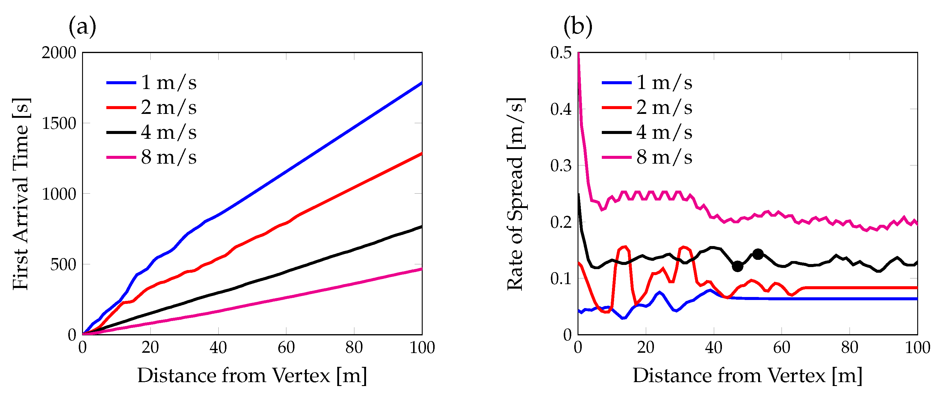
3.1. Head Fire
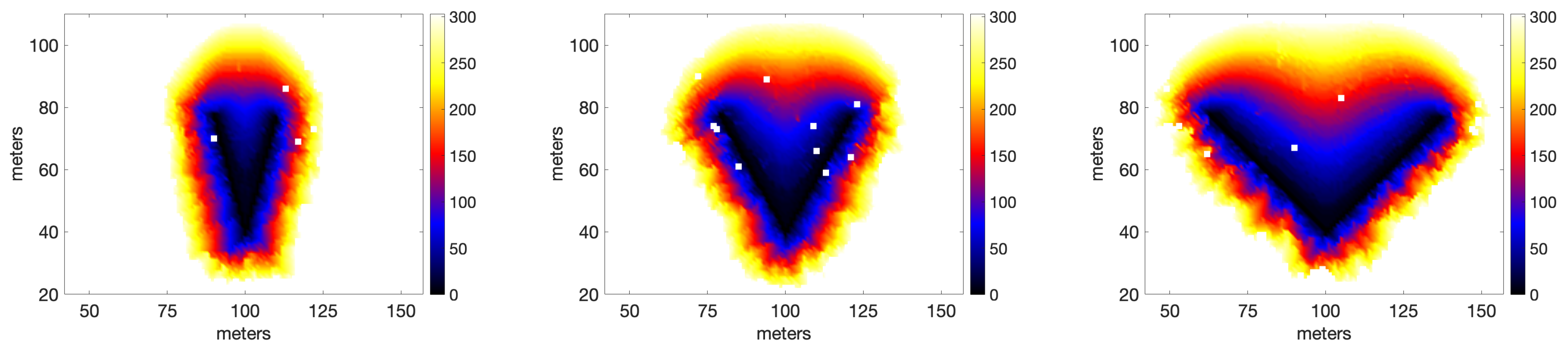
3.2. Junction Ignition Patterns
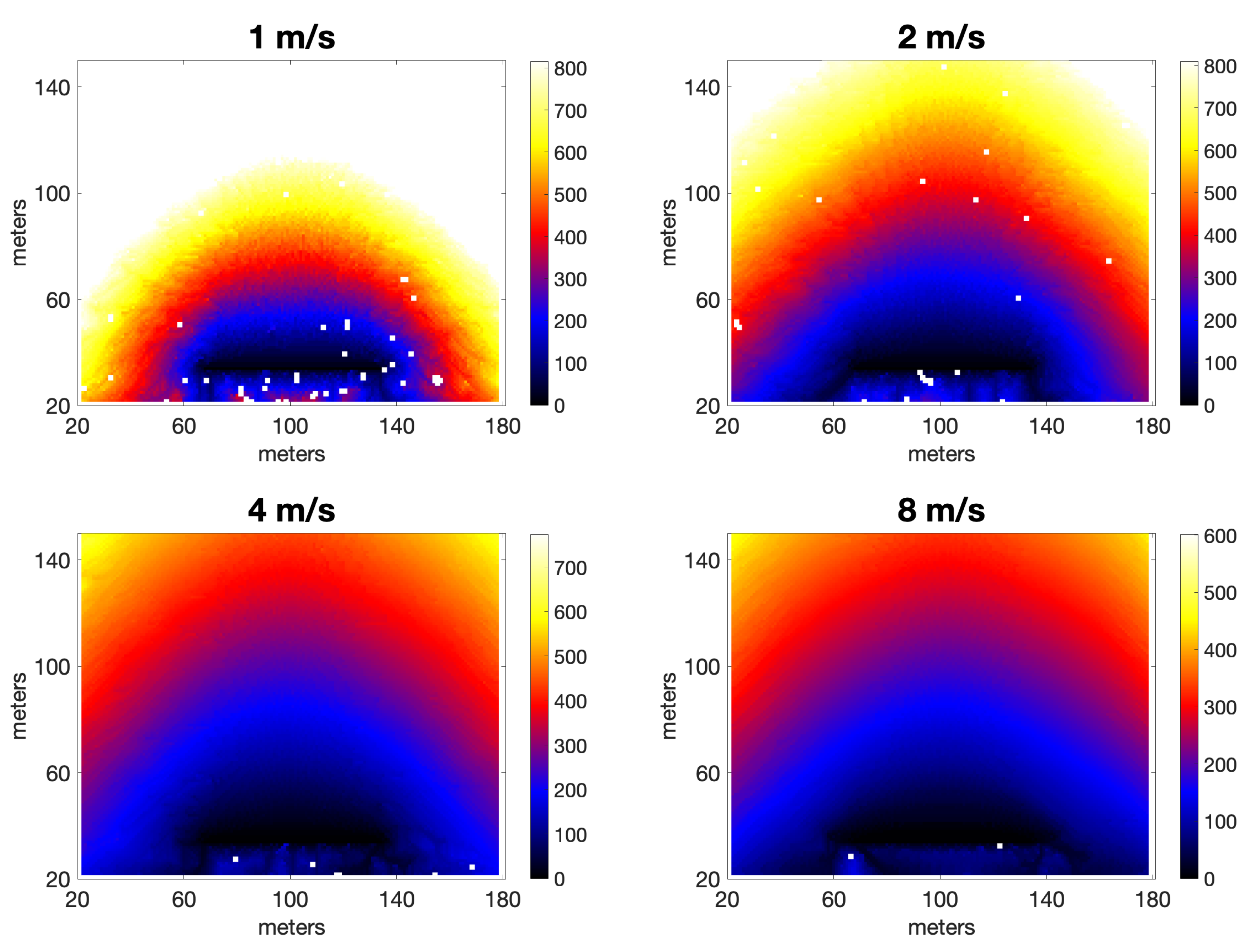
3.3. Lateral Spread in the Presence of Positive Vorticity
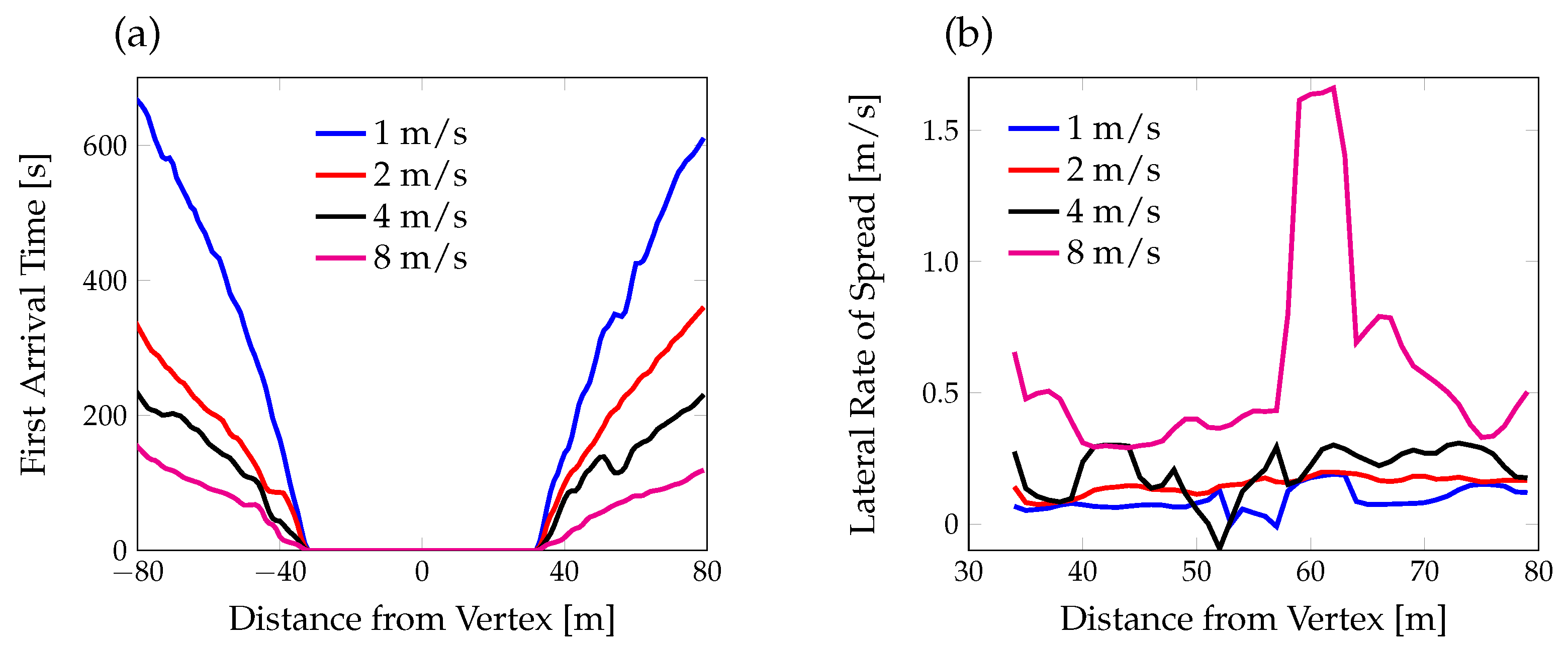
3.4. Formation of Heads by Negative Vorticity
4. Discussion and Conclusions
Author Contributions
Funding
Data Availability Statement
Conflicts of Interest
References
- Brunet, Y. Turbulent Flow in Plant Canopies: Historical Perspective and Overview. Bound. Layer Meteorol. 2020, 177, 315–364. [Google Scholar] [CrossRef]
- Sun, R.; Krueger, S.K.; Jenkins, M.A.; Zulauf, M.A.; Charney, J.J. The importance of fire–atmosphere coupling and boundary-layer turbulence to wildfire spread. Int. J. Wildland Fire 2009, 18, 50–60. [Google Scholar] [CrossRef]
- Cunningham, P.; Goodrick, S.L.; Hussaini, M.Y.; Linn, R.R. Coherent vortical structures in numerical simulations of buoyant plumes from wildland fires. Int. J. Wildland Fire 2005, 14, 61–75. [Google Scholar] [CrossRef] [Green Version]
- Clements, C.; Lareau, N.; Kingsmill, D.; Bowers, C.; Camacho, C.; Bagley, R.; Davis, B. RaDFIRE—The rapid deployments to wildfires experiment: Observations from the fire zone. Bull. Amer. Meteor. Soc. 2018, 99, 2539–2559. [Google Scholar] [CrossRef]
- Babak, P.; Bourlioux, A.; Hillen, T. The Effect of Wind on the Propagation of an Idealized Forest Fire. SIAM J. Appl. Math. 2009, 70, 1364–1388. [Google Scholar] [CrossRef] [Green Version]
- Morandini, F.; Simeoni, A.; Santoni, P.A.; Balbi, J.H. A Model for the Spread of Fire Across a Fuel Bed Incorporating the Effects of Wind and Slope. Combust. Sci. Technol. 2005, 177, 1381–1418. [Google Scholar] [CrossRef]
- Bebieva, Y.; Oliveto, J.; Quaife, B.; Skowronski, N.; Heilman, W.E.; Speer, K. Role of horizontal eddy diffusivity within the canopy on fire spread. Atmosphere 2020, 11, 672. [Google Scholar] [CrossRef]
- Clark, T.L.; Jenkins, M.A.; Coen, J.L.; Packham, D.R. A Coupled Atmosphere-Fire Model: Role of the Convective Froude Number and Dynamic Fingering at the Fireline. Int. J. Wildland Fire 1996, 6, 177–190. [Google Scholar] [CrossRef] [Green Version]
- Clark, T.L.; Radke, L.; Coen, J.; Middleton, D. Analysis of Small-Scale Convective Dynamics in a Crown Fire Using Infrared Video Camera Imagery. J. Appl. Meteorol. 1999, 38, 1401–1420. [Google Scholar] [CrossRef] [Green Version]
- Baum, H.R.; McCaffrey, B.J. Fire Induced Flow Field—Theory and Experiment. Fire Saf. Sci. 1989, 2, 129–148. [Google Scholar] [CrossRef] [Green Version]
- Eftekharian, E.; Ghodrat, M.; He, Y.; Ong, R.H.; Kwok, K.C.; Zhao, M. Numerical analysis of wind velocity effects on fire-wind enhancement. Int. J. Heat Fluid Flow 2019, 80, 108471. [Google Scholar] [CrossRef]
- Clark, T.L.; Jenkins, M.A.; Coen, J.; Packham, D. A Coupled Atmosphere Fire Model: Convective Feedback on Fire-Line Dynamics. J. Appl. Meteorol. 1996, 35, 875–901. [Google Scholar] [CrossRef] [Green Version]
- Miller, C.H.; Tang, W.; Finney, M.A.; McAllister, S.S.; Forthofer, J.M.; Gollner, M.J. An investigation of coherent structures in laminar boundary layer flames. Combust. Flame 2017, 181, 123–135. [Google Scholar] [CrossRef] [Green Version]
- Canfield, J.; Linn, R.; Sauer, J.; Finney, M.; Forthofer, J. A numerical investigation of the interplay between fireline length, geometry, and rate of spread. Agric. For. Meteorol. 2014, 189–190, 48–59. [Google Scholar] [CrossRef]
- Thomas, C.M.; Sharples, J.J.; Evans, J.P. Modelling the dynamic behaviour of junction fires with a coupled atmosphere–fire model. Int. J. Wildland Fire 2017, 26, 331–344. [Google Scholar] [CrossRef]
- Clements, C.B.; Lareau, N.P.; Seto, D.; Contezac, J.; Davis, B.; Teske, C.; Zajkowski, T.J.; Hudak, A.T.; Bright, B.C.; Dickinson, M.B.; et al. Fire weather conditions and fire–atmosphere interactions observed during low-intensity prescribed fires–RxCADRE 2012. Int. J. Wildland Fire 2016, 25, 90–101. [Google Scholar] [CrossRef]
- Hilton, J.; Sullivan, A.; Sharples, W.S.J.; Thomas, C. Incorporating convective feedback in wildfire simulations using pyrogenic potential. Environ. Model. Softw. 2018, 107, 12–24. [Google Scholar] [CrossRef]
- Sharples, J.J.; Hilton, J.E. Modeling Vorticity-Driven Wildfire Behavior Using Near-Field Techniques. Front. Mech. Eng. 2020, 5, 69. [Google Scholar] [CrossRef]
- Maynard, T.; Princevac, M.; Weise, D.R. A Study of the Flow Field Surrounding Interacting Line Fires. J. Combust. 2016, 2016, 6927482. [Google Scholar] [CrossRef]
- Bresenham, J.E. Algorithm for computer control of a digital plotter. IBM Syst. J. 1965, 4, 25–30. [Google Scholar] [CrossRef]
- Currie, M.; Speer, K.; Hiers, K.; O’Brien, J.; Goodrick, S.; Quaife, B. Pixel-Level Statistical Analyses of Prescribed Fire Spread. Can. J. For. Res. 2018, 49, 18–26. [Google Scholar] [CrossRef]
- Lareau, N.P.; Clements, C.B. The Mean and Turbulent Properties of a Wildfire Convective Plume. J. Appl. Meteorol. Climatol. 2017, 56, 2289–2299. [Google Scholar] [CrossRef]
- Johnston, J.M.; Wheatley, M.J.; Wooster, M.J.; Paugam, R.; Davies, G.M.; DeBoer, K.A. Flame-Front Rate of Spread Estimates for Moderate Scale Experimental Fires Are Strongly Influenced by Measurement Approach. Fire 2018, 1, 16. [Google Scholar] [CrossRef] [Green Version]
- Paugam, R.; Wooster, M.J.; Roberts, G. Use of Handheld Thermal Imager Data for Airborne Mapping of Fire Radiative Power and Energy and Flame Front Rate of Spread. IEEE Trans. Geosci. Remote. Sens. 2013, 51, 3385–3399. [Google Scholar] [CrossRef]
- Cruz, M.G.; Alexander, M.E. Uncertainty associated with model predictions of surface and crown fire rates of spread. Environ. Model. Softw. 2013, 47, 16–28. [Google Scholar] [CrossRef]
- Raposo, J.R.; Viegas, D.X.; Xie, X.; Almeida, M.; Figueiredo, A.R.; Porto, L.; Sharples, J. Analysis of the physical processes associated with junction fires at laboratory and field scales. Int. J. Wildland Fire 2018, 27, 52–68. [Google Scholar] [CrossRef]
- Simeoni, A.; Salinesi, P.; Morandini, F. Physical Modelling of Forest Fire Spreading Through Heterogeneous Fuel Beds. Int. J. Wildland Fire 2011, 20, 625–632. [Google Scholar] [CrossRef] [Green Version]


| (m/s) | ||
|---|---|---|
| 1 | 0 | |
| 2 | 0 | |
| 4 | 0 | |
| 8 | 0 |
Publisher’s Note: MDPI stays neutral with regard to jurisdictional claims in published maps and institutional affiliations. |
© 2021 by the authors. Licensee MDPI, Basel, Switzerland. This article is an open access article distributed under the terms and conditions of the Creative Commons Attribution (CC BY) license (https://creativecommons.org/licenses/by/4.0/).
Share and Cite
Quaife, B.; Speer, K. A Simple Model for Wildland Fire Vortex–Sink Interactions. Atmosphere 2021, 12, 1014. https://doi.org/10.3390/atmos12081014
Quaife B, Speer K. A Simple Model for Wildland Fire Vortex–Sink Interactions. Atmosphere. 2021; 12(8):1014. https://doi.org/10.3390/atmos12081014
Chicago/Turabian StyleQuaife, Bryan, and Kevin Speer. 2021. "A Simple Model for Wildland Fire Vortex–Sink Interactions" Atmosphere 12, no. 8: 1014. https://doi.org/10.3390/atmos12081014
APA StyleQuaife, B., & Speer, K. (2021). A Simple Model for Wildland Fire Vortex–Sink Interactions. Atmosphere, 12(8), 1014. https://doi.org/10.3390/atmos12081014