The Role of Heat Flux in an Idealised Firebreak Built in Surface and Crown Fires

Abstract

The disruptions to wildland fires, such as firebreaks, roads and rivers, can limit the spread of wildfire propagating through surface or crown fire. A large forest can be separated into different zones by carefully constructing firebreaks through modification of vegetation in firebreak regions. However, the wildland fire behaviour can be unpredictable due to the presence of either wind- or buoyancy-driven flow in the fire. In this study, we aim to test the efficacy of an idealised firebreak constructed by unburned vegetation. The physics-based large eddy simulation (LES) simulation is conducted using Wildland–urban interface Fire Dynamic Simulator (WFDS). We have carefully chosen different wind velocities with low to high values, 2.5~12.5 m/s, so the different fire behaviours can be studied. The behaviour of surface fire is studied by Australian grassland vegetation, while the crown fire is represented by placing cone-shaped trees with grass underneath. With varying velocity and vegetation, four values of firebreak widths (Lc), ranging from 5~20 m, is tested for successful break distance needed for the firebreak. For each failure or successful firebreak width, we have assessed the characteristics of fire intensity, mechanism of heat transfer, heat flux, and surface temperature. It was found that with the inclusion of forest trees, the heat release rate (HRR) increased substantially due to greater amount of fuel involved. The non-dimensional Byram’s convective number (N_C) was calculated, which justifies simulated heat flux and fire characteristics. For each case, HRR, total heat fluxes, total preheat flux, total preheat radiation and convective heat flux, surface temperature and fire propagation mode are presented in the details. Some threshold heat flux was observed on the far side of the firebreak and further studies are needed to identify them conclusively.

1. Introduction

For managing wildland fires, the traditional approach is to deploy firefighters to control fire with the help of different suppression techniques. With the rapid expansion of WUI, there is a need to apply more alternative approaches to different fuel modification practices that have been applied in many countries around the world [1]. The State Board of Forestry recommended the early firebreak construction in 1886 for blocking out the forest with strips of “waste” land wide enough to prevent fire crossing [2]. The fuel-break approach was first introduced in California, US in 1957, echoing the old concept of clearing strategically located areas before a fire breaks out. However, the new fuel-break concept is more about removing, controlling and replacing old vegetation with desirable vegetation cover as a part of long-term management strategies [2] to manage wildland fire. Moreover, the fuel break is used a safety zone from where the firefighters will attend a fire to protect properties at WUI.

Pimont et al. [3] validated the FIRETECH model against wind tunnel experimental data for a wind flow over canopy and fuel break, which showed some evidence of wind flow modification and gust formation across the fuel break. However, the study was limited to wind flow structure and some aspects of turbulent flow over heterogeneous canopies. It was observed that the presence of a firebreak on one hand can reduce the fire intensity, whereas on the other hand, it may increase wind velocity and gusts through the firebreak resulting in an enhanced rate of spread [3]. Dupuy et al. [4] studied the efficiency of a firebreak with the introduction of a mixture of shrubs at the ground and spatial distribution of biomass stand based on Mediterranean pine trees to study the effect of crown fire spreading towards a fuel break. The simulation establishes a connection between surface and crown fire and spreading towards a fuel break. The solid fuel elements were removed for the two sets of fuel treatment, which shows some fundamental characteristics of fuel modification effect on the firebreak. Later, Morvan [5] extended this work in detail to study the behaviour of surface fire through a firebreak illustrating the role of convective and radiative heat flux on a firebreak. The firebreak was tested for three wind velocities with the introduction of four sets of firebreak widths, which presented a little more detail about fire intensity, forefront locations and rate of spread (ROS) of fire. However, the study was limited to two-dimensional (2D) model with Reynolds Averaged Navier–Stokes (RANS) methodology.

A better insight could be obtained using large eddy simulation (LES) modelling technique in a three-dimensional (3D) model for surface fires as well as for crown fires. The consequences of fire behaviour was studied by Ziegler et al. [6] in varying intensities of conifer removal, a kind of fuel modification technique, across a range of wind speeds. The study was conducted using Wildland-urban interface Fire Dynamic Simulator (WFDS) to identify how heavier treatment on conifer forest could facilitate reintroduction of fire while also dampening the effect of wildfires on forest structure. Ziegler et al. did not focus on the role of heat flux or surface temperature.

An obvious criticism of the firebreak approach [2] is the possibility of spot fires ahead of the main fire front. In a plume, dominated fires and firebrands may be transported up to 1–2 km ahead of the main fire front. Therefore, a spot fire can spread quickly ahead of the main fire front as multiple discrete sources of fires. A post-fire investigation on the origin of the destruction of houses and buildings on Canberra fires [7] has shown that 50% of the houses were ignited by firebrands, 35% from firebrands and radiant heat and only 10% from radiant heat alone. Therefore, there is a need to address the spot fire danger at WUI when designing the firebreak system. While there is no doubt about the danger of spot fires in a real wildfire, the simulation of such spot fires in physics-based modelling is still having difficulties due to the lack of reliable firebrand generation data [8], such as firebrand numbers, sizes and shapes and thermo-physical properties.

Recently, some experimental studies [9,10,11,12] attempted to quantify the firebrand generation data, which were based on ideal conditions, for example, at no wind or low wind velocity, with constrained atmospheric conditions, and with limited influence of forest morphologies. The Lagrangian particle-based script, representing firebrands, available in WFDS/FDS that can be used for particle transportation if a reliable firebrands generation data is available, which is still missing in the scientific community. Moreover, the hot firebrands are only responsible for the spotting [12] and there is a need to have a practical ignition model that represent such spot fire scenarios. Since there is no reliable quantification method for spot fires, we are not considering the spot fire effects on this study; this may be a subject of future study.

As the firebreak studies are still limited to 2D RANS modelling techniques [4,5], this study expands it into 3D perspective for calculating more accurate turbulence flow characteristics and heat fluxes. In this study, we aim to conduct an idealised firebreak study for both surface and crown fires in LES perspective using 3D physics-based WFDS model. We focus on the role of heat flux and surface temperature in the efficacy of firebreaks. Moreover, we expand our analysis with a Byram’s convective number analysis, which is instrumental in identifying the modes of fire propagations. Different modes of fire propagation can cause different levels of contribution of radiative or convective heat flux. This study incorporates realistic surface vegetation as grass and forest trees as crown vegetation together to investigate flow dynamics, fire intensity, preheat flux after the firebreak, mechanism of heat transfer, a relative comparison of radiation and convective heat flux in more detail that can provide insight to operating agencies in designing a firebreak in WUI and in the middle of a forest.

2. Model Setup and Methodology

The study was conducted with WFDS (compatible with 6.0.0 version of Fire Dynamics Simulator, FDS developed by NIST, USA for building a fire). Vegetative fuel burning was added jointly by US Forest Department and NIST. FDS and WFDS solve governing equations for species and mass conservation equation using finite difference method with low-Mach number approximation. The energy conservation equation is not solved explicitly, rather it is defined implicitly by source terms for combustion and radiation via solving the divergence flow fields. The turbulence is modelled using LES methodology, where the large scale of turbulent structures is resolved explicitly, while the effect of subgrid scales on large scales is modelled. The details of model physics, including LES formulation, combustion model, numerical schemes and solution technique, can be found in McDermott et al. [13], McDermott et al. [14], Perez-Ramirez et al. [15], Moinuddin et al. [16], Sarwar et al. [17], etc.

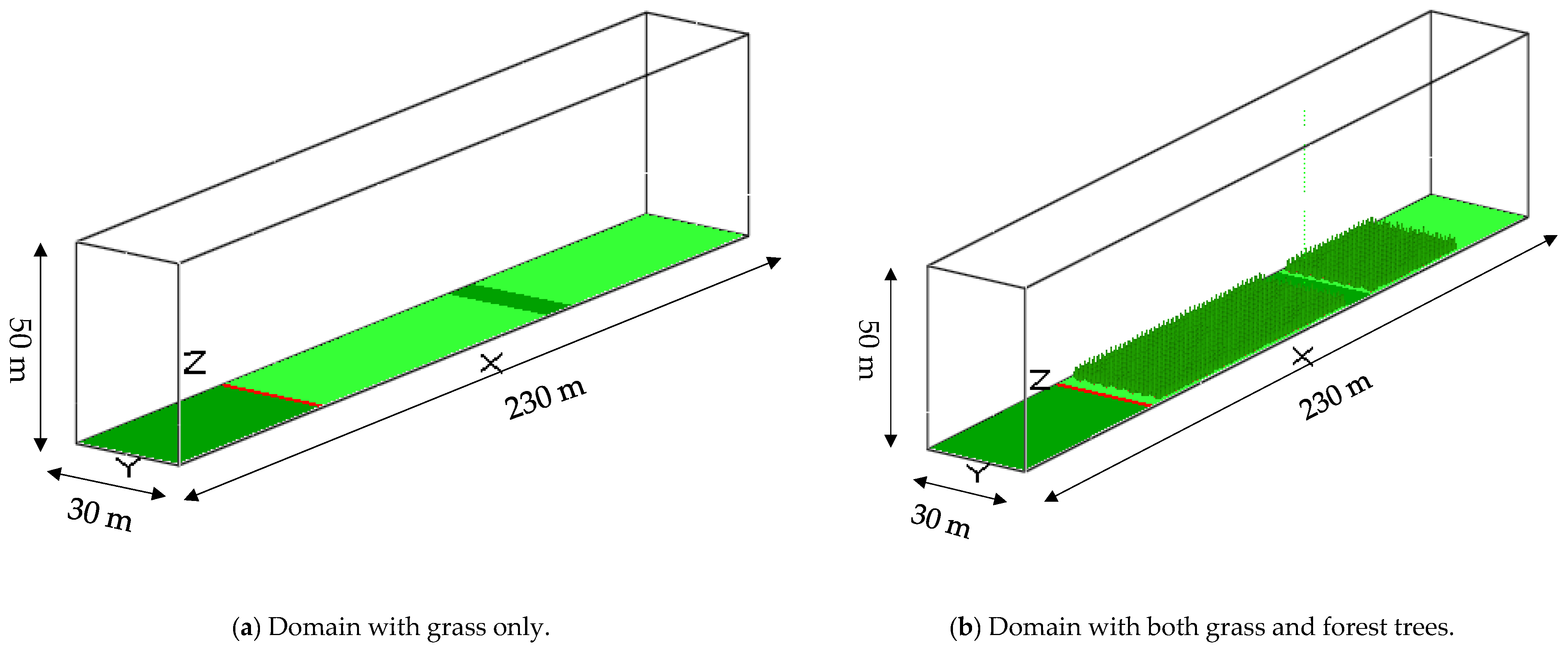
The numerical domain is 230 m long, 30 m wide and 50 m high, as shown in Figure 1. In Figure 1a, there are five sections with the following color schemes: dark green (from left) for the unburned grass, red for line fire, light green for burnable grass, dark green for firebreak and light green for burnable grass sections beyond. The burnable vegetation section is modified in Figure 1b with the inclusion of columns and rows of trees. The ignition line (red colour), 2 m depth and 30 m width, is situated at 58 m from the inlet of the domain in both cases. It represents a line fire ignited simultaneously at 620 s simulation time (after the well-developed wind field).

Adjacent to the ignition line, the light green burnable grass/forest trees starts at 60 m from the inlet and extend to 150 m. For all cases, the firebreak is set up from 150 m from the inlet of the domain. The geometry consists of 16 mesh segments with a fine uniform grid resolution of 0.25 m × 0.25 m × 0.25 m for up to 10 m height and the rest 10–50 m height was discretised by a uniform grid of 0.5 m × 0.5 m × 0.5 m size. This is because Moinuddin et al. [18] studied grid sensitivity from which the required grid size was determined for the fine mesh segments as 0.25 m × 0.25 m × 0.25 m. The total grid cell amounts in x, y and z-direction were 2240, 840 and 1200; respectively.

The grass vegetation and thermo-physical parameters are shown in

Table 1. Vegetation, thermophysical, pyrolysis, and combustion parameters.

Parameters Input (WFDS)	Values	Units	Description
Grass vegetation
VEG_SV	9770	m−1	Surface to volume ratio
VEG_MOISTURE	0.063	%	Moisture
VEG_CHAR_FRACTON	0.17		Vegetation char fraction
VEG_DRAG_COEFFICIENT	0.125		density
VEGE_DENSITY	440	kg	Vegetation density
VEG_DEGRADATION	Linear		Degradation model
EMISSIVITY	0.99		Emissivity index
VEG_HEIGHT	1.0	m	Vegetation height
VEG_LOAD	1.2	kgm−2	Vegetation load
HEAT_OF_COMBUSTION	16400	kJkg−1	Heat of combustion
SOOT_YIELD	0.008	gg−1	Soot
HUMIDITY	40	%	Relative humidity
TMPA	30	°C	Ambient temperature
Tree canopy (CONE)
CROWN_WIDTH	2.0	m	Width of the tree
CROWN_BASE_HEIGHT	0.5	m	Base height of tree
TREE_HEIGHT	4	m	Tree height
Tree Trunk (CYLINDER)
CROWN_WIDTH	0.3	m	Width of the tree trunk
CROWN_BASE_HEIGHT	0.0	m	Base height of tree trunk
TREE_HEIGHT	0.5	m	Height of tree trunk

, which are similar to the previous study of Moinuddin et al. [18,19] and Sutherland et al. [20] except the vegetation height that is mentioned in the next paragraph. For the forest vegetation, tree canopies and tree trunks are defined as cone and cylindrical geometry, respectively as shown in Table 1. The tree model is set up with thermophysical parameters similar to the study of Moinuddin et al. [19] but the tree dimensions are different.

A symmetry plane (Mirror) boundary condition is applied on the left, right and top boundaries, while an OPEN boundary condition is applied on the outlet plane (at the end of x_max plane). The inlet velocity was prescribed according to a 1/7th power law wind profile in a neutral atmospheric boundary layer (ABL) following Morvan et al. [21]. To reduce the spin-up time and ground length (prior to the ignition line) for the wind development as well as for initial perturbation, the Synthetic Eddy Methodology (SEM) proposed by Jerrin et al. [22] was applied for introducing turbulent flow in the domain. We used N_EDDY = 200, L_EDDY = 1.0 based on the domain size, grid, and eddies.

We artificially injected eddies to the domain to make sure that the initial perturbation to the flow field and the subsequent development of wind flow take place quickly. The cases, shown in

Table 2. Simulated cases with break status.

Velocity (m/s)	No of Cases	Break Width (LC)	Vegetation before Break	Vegetation after Break	Time to Reach Fire at Break (sec)	Successful Break Width (m)
2.5	4	5, 10, 15, 20	Grass	Grass	865	10, 15, 20
2.5	4	5, 10, 15, 20	Grass + forest	Grass + forest	765	15, 20
2.5	4	5, 10, 15, 20	Grass + forest	Grass	765	15, 20
6.0	4	5, 10, 15, 20	Grass	Grass	834	10, 15, 20
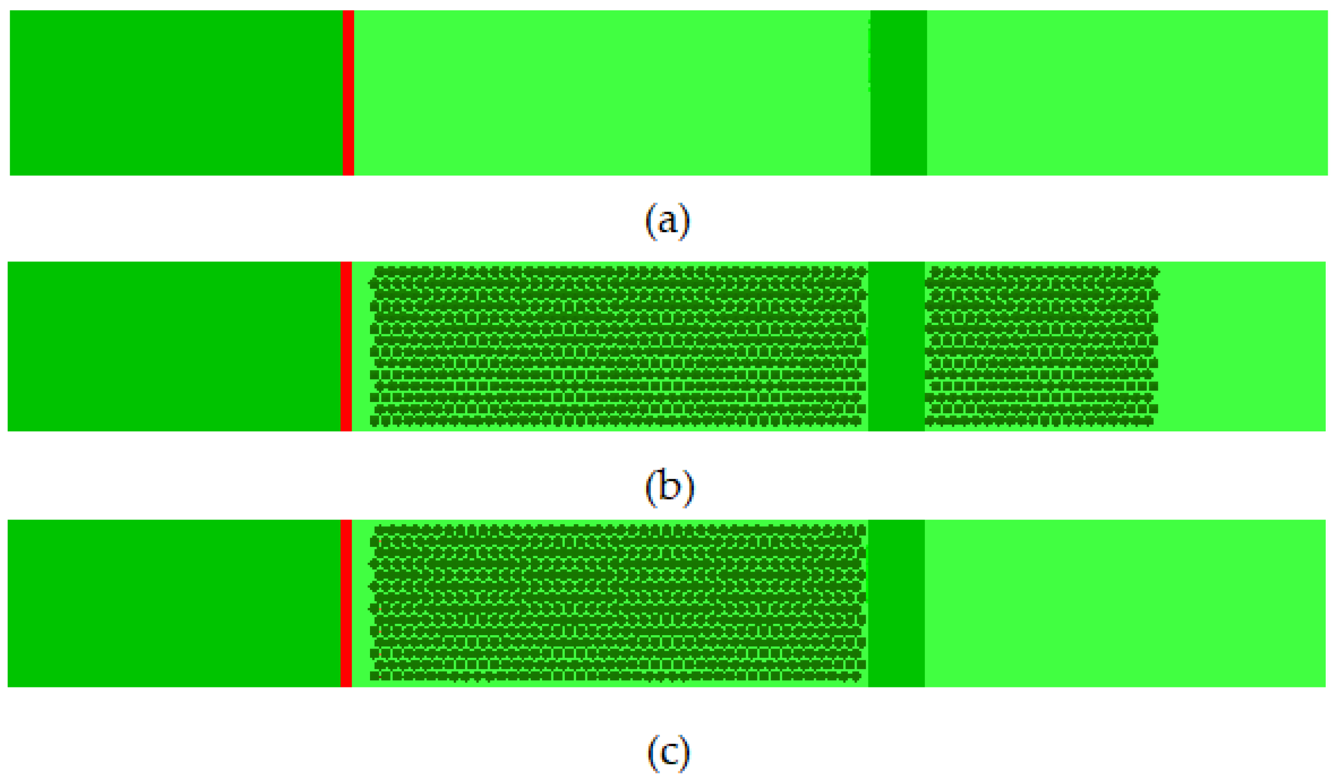
12.5	4	5, 10, 15, 20	Grass	Grass	760	15, 20

, were set up for three driving wind velocities: 2.5, 6.0 and 12.5 m/s (at 2 m above the ground at inlet) while the vegetation layout was varied as shown in Figure 2a–c. In this study, a grass height of 1.0 m was chosen for studying the effect of tall grass. According to Moor [23], in Australia major tall grass can be >90 cm. The fuel load was 12 t/ha (1.2 kg/m2). The trees of this study represent a typical Australian Chapparal vegetation composed of broad-leaved evergreen shrubs, bushes, and small trees. The vegetation layout is shown in Figure 2a–c. The vegetation layout is modified with the inclusion of forest vegetation on the burnable section before and after the firebreak. There are 20 cases simulated in total as shown in Table 2 for 4 break widths (Lc): 5, 10, 15 and 20 m.

The wind field plays an important role in both combustion and heat transfer processes. The ABL development is allowed for sufficient time in simulations to adjust with the turbulent flows at the top of the grass. For each velocity case, 2.5, 6.0, 12.5 m/s with grass as burning fuel and 2.5 m/s cases with forest trees with grass underneath, the streamwise mean velocity is shown in Figure 3. For each case, the fully developed wind field is used in the simulation. The stream-wise mean velocity, u (m/s), is plotted against the height of the domain for up to 10 m in height to see the U₁₀ velocity in the domain. The velocity profiles show an early inflection point at the top of the grass height of 1 m and then developed a vertical profile with some deflection at different x locations. The profiles at xd = 30, 40, 50 and 60 are found subsequently undergoing a trend of higher drag force leading to increased Kelvin-Helmholtz shear instability similar to the study of Dupont and Brunet’s [24] coherent structures in canopy edge flow. Therefore, the ABLs are generally well-developed, as shown in Figure 3, and the velocity profiles are matching at different x locations except for some variation in locations from 3 to 5 in grass height (especially with grass and forest case), where the velocity is varying each other due to the drag forces with respective x locations.

3. Results and Discussion

The simulation results are presented in both quantitative and qualitative manners where applicable. Although the efficacy of the firebreak is fundamental aspect to this study, the characteristics of heat flux, fire intensity, and temperature are also vital to understand the behaviour of wildfires in the presence of a firebreak built in WUI or elsewhere. In the following subsections, the results of twenty simulations are summarised highlighting the role of heat flux in an idealised firebreak built in surface and crown fires.

3.1. Effect of Firebreak

The purpose of the firebreak is to stop fires that are propagating through a specific region. This is done by various fuel modification techniques, for example, a variety of fuel gap starting with homogenous to heterogenous or absence of any vegetation. These fuel modification techniques can develop various degrees of wind gust, recirculation that would make the modelling more complex. However, for this study, the firebreak is defined by unburned grass to study the effect of heat flux in the firebreak region irrespective of any complex fuel modification. We are interested in the characteristics of heat flux and temperature on the far side of the firebreak regions from the inlet of the domain, where the burning of vegetation and the failure of the break may occur.

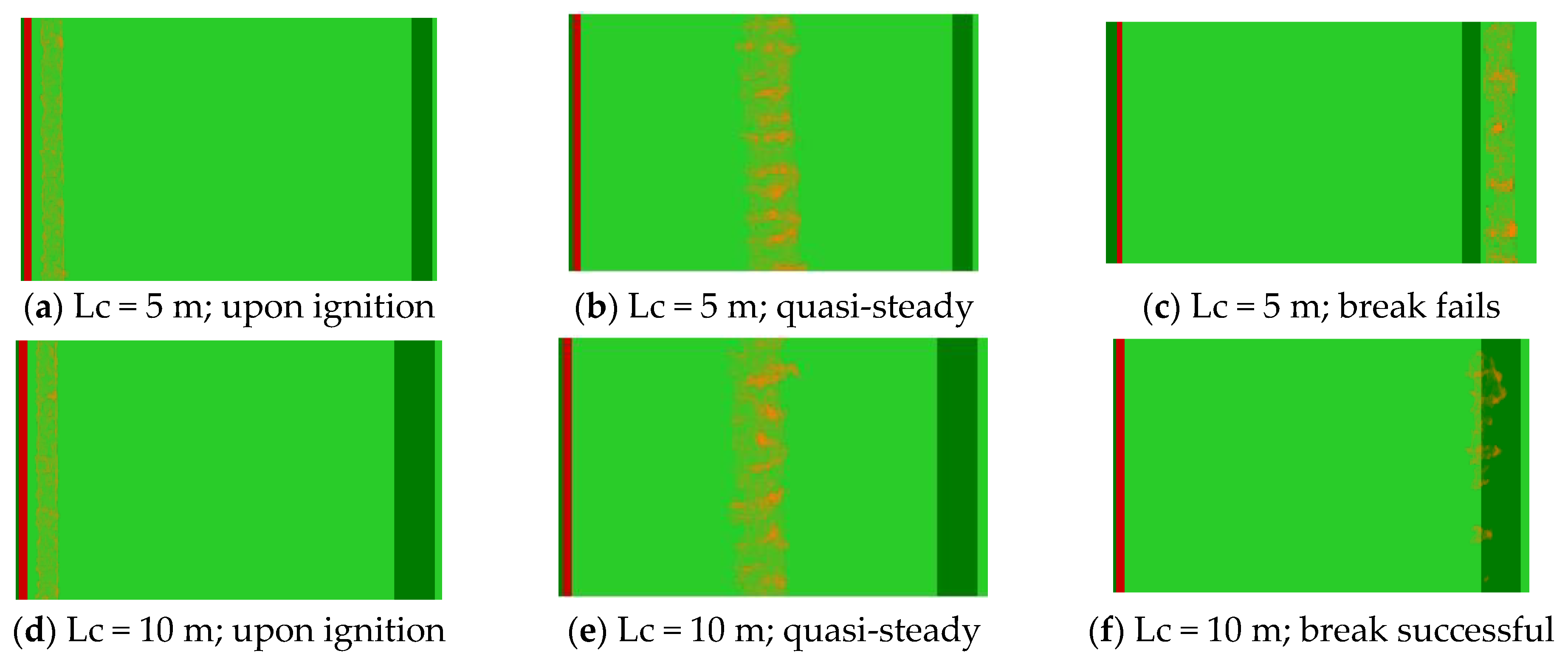
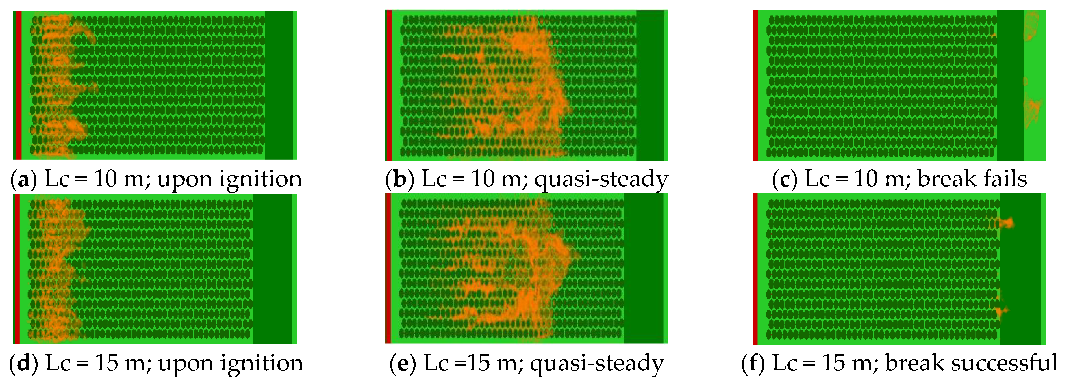
The contour plot of heat release rate per unit volume (HRRPUV) as shown in Figure 4 and Figure 5 are presented here to demonstrate the firebreak failure and success with two break widths in each case. The contour plots are shown with a fire cut-off value of 80 kW/m³. HRRPUV often represents flame structure. In the 2.5 m/s velocity cases, unsuccessful and successful break widths were at 5 m and 10 m, respectively. Similarly, the contour plots of the 2.5 m/s case with grass and forest tree cases are shown in Figure 5, where the break was successful at 15 m width. For the same velocity of 2.5 m/s, the forest fire was stronger in terms of fire intensity, heat flux (discussed below), and it took a 15 m break width to stop the fire.

Similarly, for all the cases, we have viewed the HRRPUV in Smokeview to identify the break status, whether it fails or succeeds. With a specific break width, if the fire is unable to continue vegetation burning on the opposite side of the break, the break width is assumed to be successful; otherwise, it was flagged as unsuccessful. A list of break status is shown in Table 2, which shows that a minimum break width of 15 m is needed to stop the fire crossing the firebreak for the cases simulated in this study. Although the vegetations of this study was different from the study of Morvan [5], a minimum safe break width was found 15 m in both studies.

3.2. Heat Release Rate

The HRR indicates the potential risk and vulnerability magnitude in both building and wildland fire. It is also a measure of the fire size in kW or MW. In the wildfire literature, often fireline intensity, I (HRR divided by fireline length) is used. HRR or I can vary based on many parameters such as fuel density, wind velocity, moisture content, the heat capacity of vegetation, slope, or terrain features, and some of them were investigated by Dupuy et al. 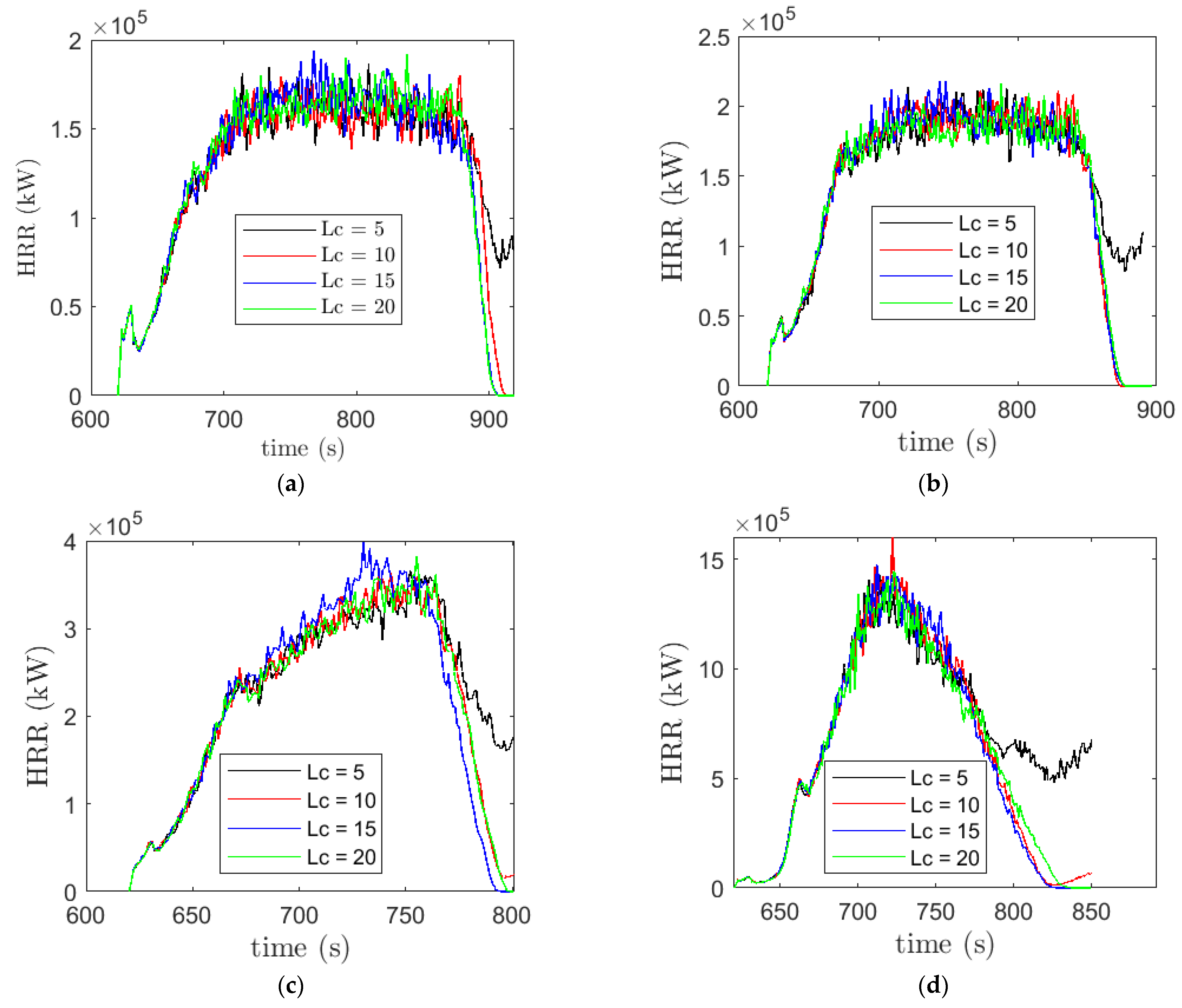[18]. In this study, we have evaluated growth and decay of HRR in both surface and crown fires for the three velocities as shown in Figure 6. For all the cases, the HRR first steadily grows upon ignition. For the lower velocity cases, 2.5 and 6.0 m/s; we found that the HRR grows to roughly quasi-steady values, while the other two sets had a sharp increase of the HRR. The quasi-steady period is very short for the 12.5 m/s cases and there is no quasi-steady period for grass and forest cases.

Among the grass cases, as expected [18,25], the HRR increases with the increase of velocity from 2.5 m/s to 12.5 m/s. For the event of a successful break, the HRR falls to zero as the fire is extinguished and could not propagate to the other side of the break. The transition from grass to forest fire cases (Figure 6d) is highly fire-intensive, which shows a triangular-shaped distribution of the HRR. Moreover, the HRR does not change much before the firebreak regions with varying break widths and the HRR profiles collapse onto each other at Lc = 5, 10, 15 and 20 m before the break. At the same time, the HRR starts to grow after the firebreak for the unsuccessful cases (Figure 6).

In the following subsections, we discuss heat fluxes in detail, which are directly linked to the HRR as the heat flux largely depends on the HRR. However, we will limit our discussion to case with successful break width and the other one with unsuccessful break width for each velocity. To see the effect of break widths on preheat fluxes, the results are presented for all the break widths.

3.3. Mechanism of Heat Flux

To understand the role of radiation or convective heat flux on vegetation burning, the contour plot of the heat flux is presented in Figure 7 and Figure 8 for the two sets of velocity cases; 2.5 and 12.5 m/s.

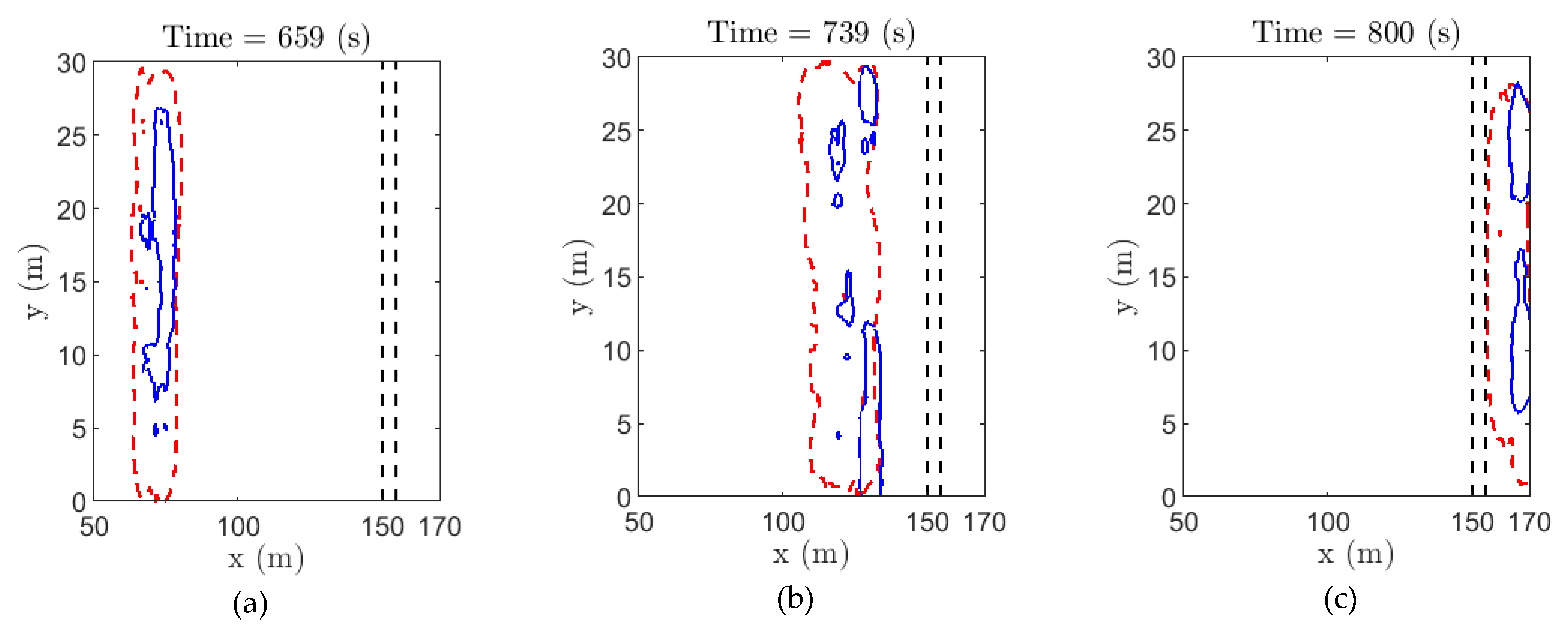
As the heat flux varies due to wind velocity, atmospheric conditions and thermophysical parameters of vegetations, there is no physical threshold value for the heat flux. We have filtered data to find the trailing edge of pyrolysis regions, where data are normalised to generate the range from 0 (T < 400) to 1(T ≥ 400) and the contour plots are presented at 0.5, where T stands for the temperature of the flame. Therefore, 50% of the heat transfer occurs inside of the contour. The contour plots are taken at random time steps to show the changes in time and space of heat transfer in the numerical domain up to firebreak regions. In the beginning, the convective (blue) and radiative heat flux (red) contours are overlapping each other (Figure 7). The convective flux contours lie ahead of radiative contours at the end of 800 s. At a higher velocity case (Figure 8), as of 12.5 m/s, the convective contours clearly lie ahead of radiative contours during all the times. These results are demonstrating that the convective heat flux is leading over the radiative heat flux as the driving wind velocity is increasing. With the higher the driving wind velocity, the more propagation becomes wind-driven and convective heat flux becomes more relevant.

3.4. The Role of Temperature in Firebreak

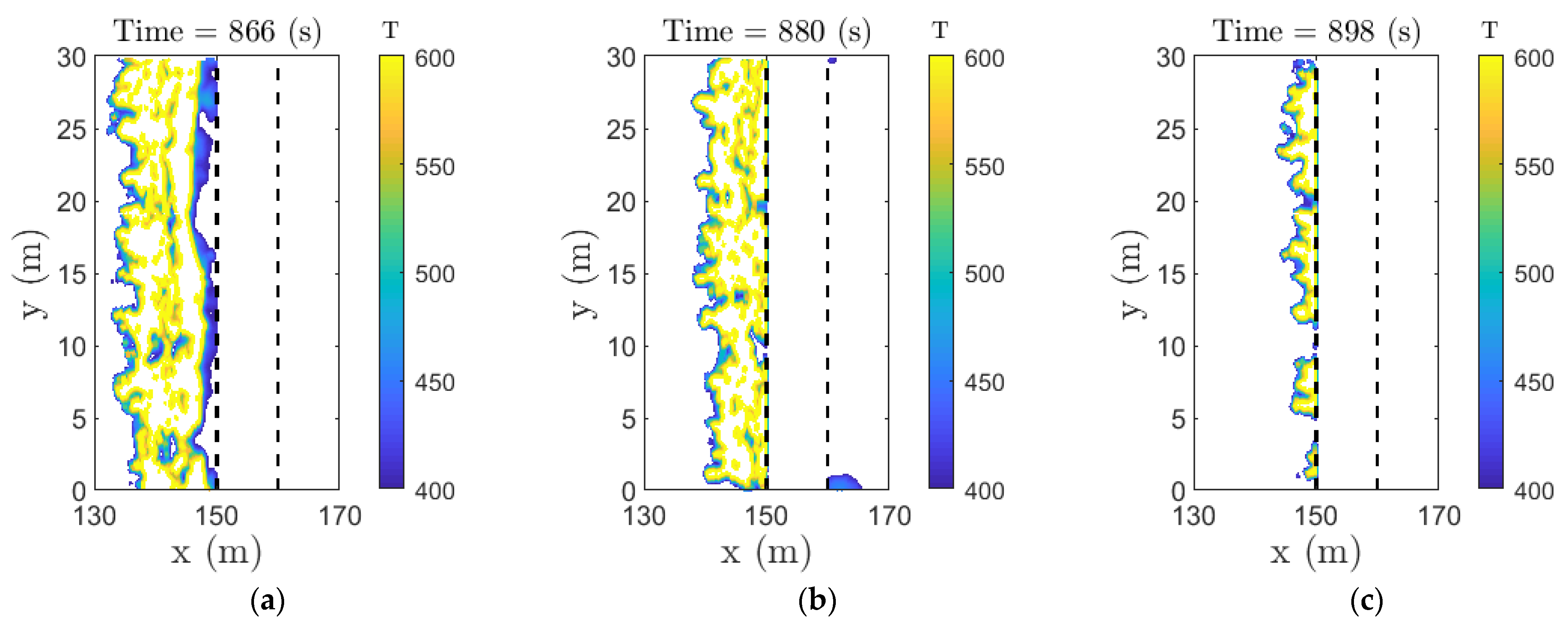
The surface temperature is an indicative of heat transfer from flames to the surrounding fuels. Whether it is due to radiative or convective heat flux, the surface temperature is a single parameter that can be useful to measure extend of heat transfer to the vegetation that may reach pyrolysis temperature. The contour plot of temperature is shown in Figure 9 and Figure 10 for the two break widths, 5 m, and 10 m, respectively, for the 2.5 m/s velocity cases. The contour data are filtered for a limit of 400–600 K to see whether the vegetation is hot enough to continue the fire propagation. The break was failed at 5 m width at a velocity of 2.5 m/s (Figure 9), where we observe the threshold temperature appearing on the other side of the firebreak. On the other hand, the firebreak was successful at a break width of 10 m (Figure 10), which shows only a few dots of temperature around 400 K to appear in the other side of the break at a time of 880 s. However, this discrete temperature value of around 400 K was not sufficient to ignite the required amount of vegetation on the other side of the break. It demonstrates that the fire did not propagate on the side of the break, even though the temperature was around 400 K.

3.5. Heat Flux in Vegetation Burning

Heat flux characteristics are important to understand the efficacy of a firebreak in a real case scenario. In fact, the vegetation is preheated by heat flux at the other side of the break, which in turn ignites the vegetation when the temperature reaches the pyrolysis temperature of fuels. The total radiation and convective heat flux are shown in Figure 11. The time to reach the firebreak is labeled by dashed lines. For each failure or successful break width, the fire’s time to reach the firebreak was 865, 765, 834 and 760 s for the different velocities as shown in Table 2.

The total convective heat flux was higher than the corresponding radiative flux for all the cases. For the velocity 2.5 m/s, grass with forest tree cases, the heat fluxes are observed to be higher than in the other cases (Figure 11d). For the higher velocity of 12.5 m/s, the difference between the radiative and convective heat flux lessened compared to all the other cases due to the increase in radiative heat flux.

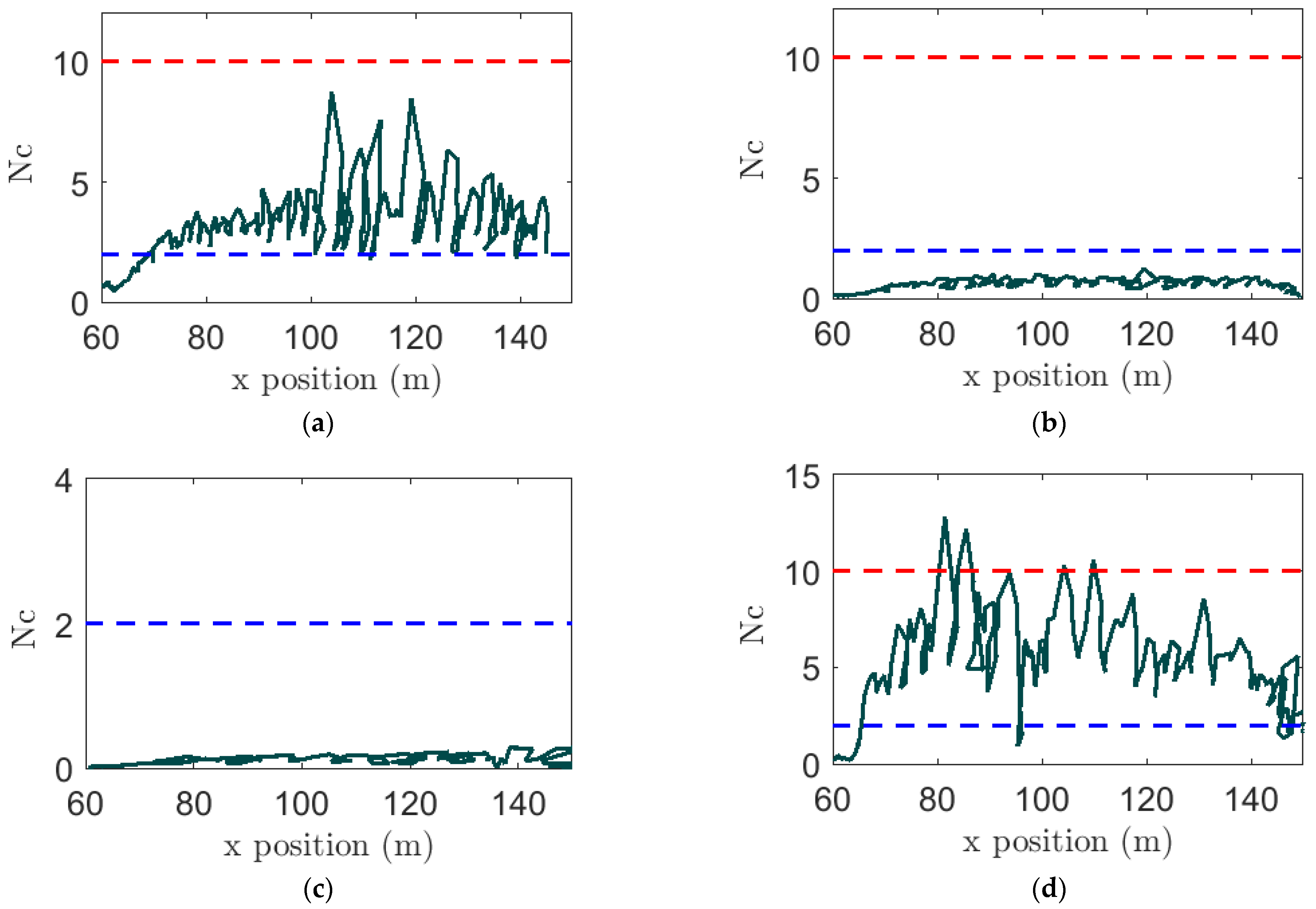
To investigate the fire characteristics and associated heat flux, we calculated Byram’s convective number (N_C) as shown in Figure 12. The equation for N_C, which is the ratio between buoyancy and inertia forces, is defined [5,20] as the following:

$${\mathrm{N}}_{\mathrm{C}}=\frac{2\mathrm{gQ}}{{\mathsf{\rho }\mathrm{C}}_{\mathrm{p}}{\mathrm{T}}_0{\left({\mathrm{U}}_{10}-\mathrm{ROS}\right)}^3}$$

(1)

Here U₁₀ is the velocity at 10 m height, which is far from the flame, taken here as the time averaged velocity from Figure 3. The fire intensity, Q was computed as globally averaged heat release rate (HRR) divided by the fire line length [20]. The other parameters used to compute N_C were: g is acceleration of gravity (9.81 m/s²), $\mathsf{\rho }$ is air density (1.171 kg/m³), ${\mathrm{T}}_0$ (300 k) and ${\mathrm{C}}_{\mathrm{p}}$ (1010 J/kg.k) are temperature and specific heat of ambient air, the ROS is rate of fire spread. We determined fire front locations, x, as a function of time using an in-house MATLAB code. The location is when the surface temperature is first reached at 400 K or above. Then, by taking the time derivative of fire front location, the ROS is calculated [18].

According to wildfire data and experimental fires, Morvan and Frangieh [26] determined that if N_C is less than 2, the fire is considered as wind-driven and if N_C is more than 10, the fire is buoyancy-driven. If N_C values fall between 2 and 10, the fire is in the transition region and the fire is neither wind nor buoyancy driven. There is a possibility of surge-stalled regime [27,28], where fires oscillate between wind-driven, and buoyancy-driven modes. For the higher velocity cases, 6.0 and 12.5 m/s, we found N_C values less than 2 (Figure 12b,c), which is reflective of wind-driven propagation. For the lower velocity 2.5 m/s cases, we found the N_C values lie in between 2 and 10, which is reflective of the transition regime (Figure 12a,d). When the fire propagation is transitory in nature, either convective or radiative heat flux can be higher and in this study the cases with 2.5 m/s wind velocity; at times, higher convective heat flux is observed (Figure 11a,d).

3.6. Preheat Flux after Firebreak

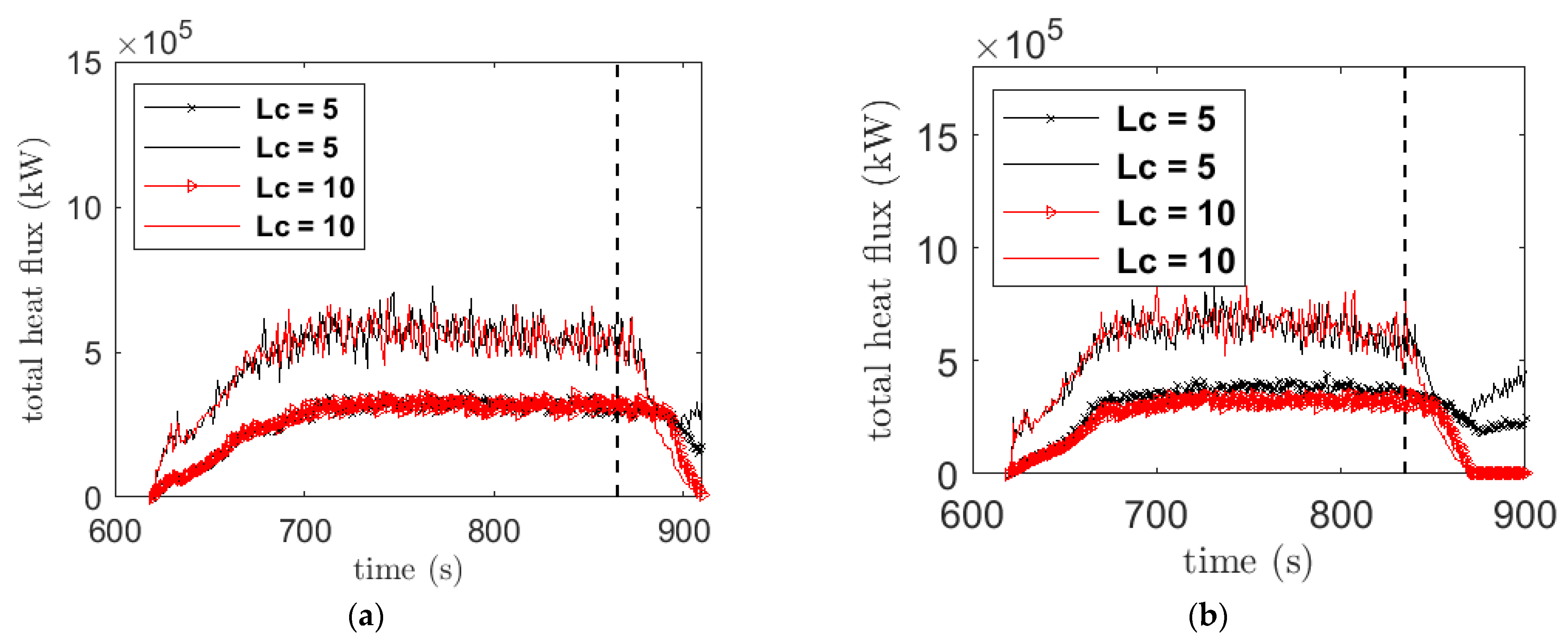
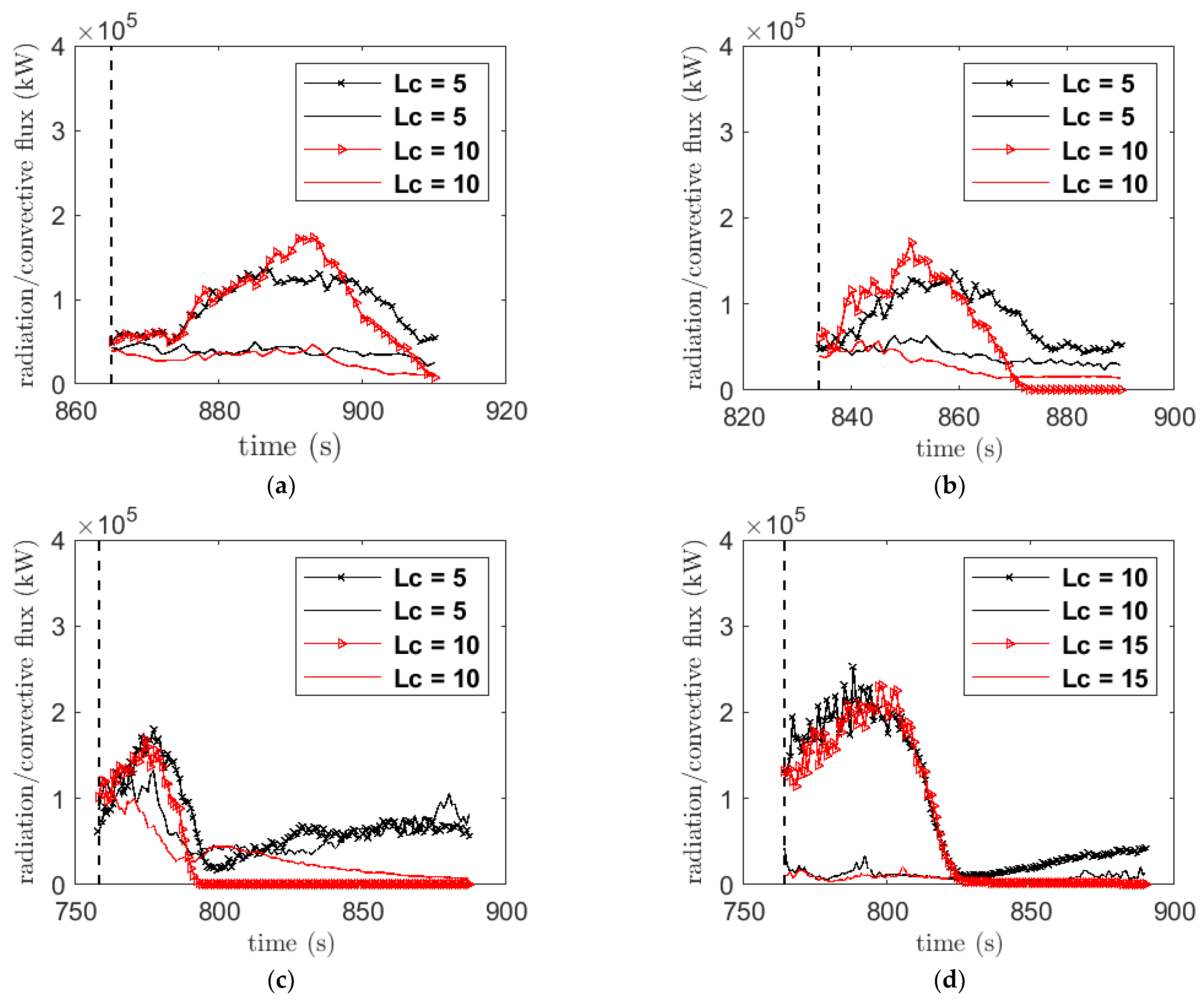
The preheat flux is defined as the amounts of heat flux transferred to burnable vegetation ahead of the fire front location, while the temperature is still below the pyrolysis temperature (400 K) of vegetation. The preheat flux after firebreak indicates the strength of heat flux at break regions, which is useful to understand the effectiveness of break widths. The preheat flux is shown in Figure 13 for 16 cases (excluding the set with forest on both sides of the firebreak). The preheat fluxes are shown for all the four break widths, which show variation of fluxes with respect to widths as expected. For velocity 2.5 m/s, the successful widths were 10, 15 and 20 m, which is reflected in the preheat flux results although at Lc = 10, the heat flux was relatively higher at some point compared to the Lc = 5 case, but the fire was unable to cross the break width. For velocity 6.0 m/s, the successful break widths were also 10, 15 and 20 m but the preheat flux at Lc = 10 was following similar trend to the higher break width cases (Figure 13b). Interestingly, this difference in flux profiles with 2.5 m/s and 6.0 m/s cases at Lc = 10 may be due to the mechanism of heat transfer as depicted in Figure 12a,b, as these two cases represented different mechanisms of heat transfer process. For the cases with 12.5 m/s and 2.5 m/s with forest trees, in Figure 13c,d, there is a smooth variation of fluxes with respect to their break widths and the successful break widths in these cases were 15 and 20 m; respectively. The peak total preheat flux, which includes both radiative and convective heat flux, is of order 3 × 10⁵ kW, which is much lower than the combined radiative and convective fluxes as shown in Figure 11 before the break regions. For the unsuccessful firebreak cases, it appears that the break fails when preheat flux reaches above the range of 0.5 × 10⁵~1 × 10⁵ kW as opposed to successful break cases when preheat flux falls below 0.5 × 10⁵ kW. This preheat flux range can be useful in designing a real firebreak.

To see the contributions of radiative and convective preheat flux, we presented these separately in Figure 14. However, the convective heat flux is higher elsewhere before the break regions; the situation is reversed when the fire reached the firebreak. The total radiative preheat flux is much higher than the corresponding convective flux in a typical firebreak region. This should be considered when designing such a firebreak in a practical application.

4. Conclusions

A physics based LES simulation has been conducted in WFDS for testing the efficacy of firebreak built in surface and crown fires. The simulation domain and grid resolution were chosen based on previous studies so that the results are independent of the computational domain and grid. Before igniting the fire, the simulations were allowed sufficient time to establish a stable ABL in the domain. For each velocity and vegetation layout, a stable wind field was ensured through an investigation of the mean velocity field in streamwise directions. It was found that the wind field for the 5 sets of simulations is well developed with some exceptions due to the presence of grass and forest trees as mentioned earlier.

The study was conducted for a range of wind velocities, 2.5~12.5 m/s, for studying the mechanism of heat transfer that may occur due to flow dynamics associated with different velocity fields. The efficacy of firebreaks has been tested for 20 simulations with four varying break widths for each velocity and vegetation layout. It is found that the minimum safe break distance varies with both velocity and vegetation layouts depending on their heat transfer characteristics. The quantifiable safe break distances were determined for each case, and it was found that the minimum threshold break distance of 15 m is enough to contain the fires. Note that the efficacy of the firebreak may be compromised due to some extreme conditions, such as, fuse effect on steeply sloping landscape, fires in heavy and hazardous fuel in intervening land, and spot fires ahead of the main fire front. Moreover, the presence of hills or ridges on the landscape, fuel heterogeneity, and extreme weather conditions may affect the efficacy of the firebreak. Apart from these extreme conditions, the firebreak may provide a significant support for managing fires at WUI either by completely stopping or slowing down the spread of fires, which may save properties and lives.

A detailed heat flux scenarios are presented, including total heat flux, preheat flux, mechanism of radiative and convective heat fluxes. The HRR values are indicative of the heat flux scenarios. The highest HRR is found in crown fires as the forest fire is supported by underneath grass vegetation fires. The Byram’s convective number is calculated for each case, which justifies mechanisms behind the heat flux values, the dominance of radiation, or convective terms in the fires. Even though the minimum safe break distance of 15 m is enough to contain fires, the operating agencies should be careful in selecting safe break distances as there is an uncertainly of wind or buoyancy-driven flow in the transition region. The preheat flux values were determined to understand the limiting range of preheating flux that might be important for designing a firebreak. However, more studies are needed to determine a quantifiable preheating flux value that can be used in firebreak design.

The main findings of this study are:

• The minimum effective break distance is found to be 15 m in an ideal situation irrespective of any extreme conditions mentioned earlier. However, the heat flux characteristics must be considered for the safety of the firefighters and the owner of the property.
• The convective heat flux is a dominant mode when the flow is wind-driven, as expected. In transition mode also in the cases studied here, where the dominant heat transfer mechanism is the convective flux.
• The preheat flux after the break shows some threshold values in the range 0.5 × 10⁵~1 × 10⁵ kW after which the fire was stopped. However, more studies are needed to justify the threshold values so they can be useful for designing a real firebreak.
• The convective heat flux increased with the increase of wind velocity in all the cases, with the exception of after the firebreak regions, where the radiation heat flux was higher than the convective flux.
• For the successful break, despite the high temperature, more than 400 K, was found on the other side of the break, the fire could not continue. However, more studies are needed to suggest any temperature threshold for the successful firebreak.

Overall, the role of heat flux in vegetation burning is successfully identified by physics-based simulation. This study can be helpful to understand the fire behaviour at firebreaks and the fire management agencies can use this knowledge for designing, planning and building of firebreaks in WUI. Further investigations using physics-based models, such as in WFDS, would help to understand the efficacy of breaks with the inclusion of more complex scenarios, such as wind gust, wind recirculation and fuel gap. In addition, a Lagrangian particle-based firebrand model (which is available in WFDS) can be used for simulating spot fires once a set of reliable firebrand generation data is available.