Assessing Hydrological Impact of Forested Area Change: A Remote Sensing Case Study

Abstract

The interaction between precipitation and vegetation plays a significant role in the formation of runoff, and it is still a widely discussed issue in hydrology. The difficulty lies in estimating the degree to which a forest influences runoff generation, especially flood peaks, on the one hand, due to the small amount of information regarding the evolution of the forest area and density, and, on the other hand, the correlations between these indicators and the runoff and precipitation values. The analysis focuses on a small basin in the mountain region of Romania, the upper basin of the Ruscova River located in northwestern Romania. In this river basin, there is no significant anthropic influence, other than the intense deforestation and reforestation actions. Using satellite images captured by Landsat missions 5, 7 and 8 for the period 1985–2019, the forest canopy density vegetation index was extracted. Using a gridded precipitation dataset, a hydrological model was calibrated based on three scenarios to assess the impact of forest vegetation on the runoff. Analysis of the results of these models conducted on scenarios allowed us to deduce a simple equation for estimating the influence of forest area on maximum river flows. The analysis showed that even small differences in the forest surface area exert an influence on the peak flow, varying between −5.28% and 8.09%.

1. Introduction

Land use and land cover change (LULCC) represents one of the most important factors that alters the natural runoff regime. Andréassian (2004) [1], citing Pliny the Elder, from the first century AD, already identified a correlation between forest removal and the subsequent increase in streamflow. At the global level, many researchers have tried to estimate/evaluate the impacts of LULCC on the evolution and changes in runoff regimes [1,2,3,4].

Forests play an important role in the natural water balance, influencing runoff and generally regions’ water resources. Anthropogenic deforestation and reforestation are among the most important land use and land cover changes worldwide [5]. In forested catchments, the climate change impact is significant since a rising temperature can reduce trees’ vitality even though precipitation amounts do not change [6]. A recent study found that, in some cases, changes in land use influence the surface runoff response more significantly than climate change [7].

According the PannEx White Book, it is particularly vital to study the effect of deforestation on catchment runoff [8]. Understanding the influence of LULCC on river flow regimes is important from many points of view, such as sustainable catchment management, establishing a correlation between floods and deforestation and assessment of drought periods.

A significant part of the worldwide weather-related natural hazards are generated by extreme rainfall, since their impact has become more and more costly and dangerous through the last century [9,10]. Most climate scenarios estimate an increase in extreme precipitation events’ intensity and frequency [11,12]. A higher intensity of rain would lead, in many parts of Europe, to an increased risk of floods.

In Romania, as one of the most flood-prone countries in Europe [13], floods are among the most important natural hazards, causing significant direct and indirect, tangible and intangible damages. They are generated by stronger intensity precipitation events that have become more frequent over recent decades [12].

Since both changes in the area covered by forests and precipitation variations are fundamental factors of runoff regime changes, in this paper, we aimed to estimate their impact on the natural discharge, referring, here, especially to the influence of forests on flood peaks. There are some approaches for LULCC analysis which assess the forest canopy density (FCD) by remote sensing [14]; for this study, forested areas were important. Numerous studies around the world have shown a direct correlation between forest-covered area and flood frequency [15], with a significant impact at the local scale (head waters, small basins) [16,17].

Numerous authors have tried to link land use to flood wave attenuation by using HEC-HMS (Hydrologic Engineering Center-Hydrologic Modeling System), or SWAT (Soil & Water Assessment Tool) in conjunction with the NDVI (normalized difference vegetation index) or LAI (leaf area index) [18,19].

Analyzing the effect of changes on land use as well as the impact of these changes on hydrological systems, Dwarakish et al., 2015 [20] performed a comprehensive analysis of several hydrological models. To determine the patterns for land use changes, they considered the evolution of human society and the growing need to expand the agricultural land area. On the same topic, another author considered that climate change and the increase in agricultural areas against forested areas will have an impact on available water resources [21].

Lately, in Romania, there has been increasing emphasis on green measures to protect settlements from the effects of floods, and more and more funds have been invested for the creation of flood control reservoirs, relocation of dikes or measures regarding the restoration of aquatic habitats and species, measures for high waters to have more transit space and aquatic life to develop in these areas, the creation of wetlands, etc. [22,23,24]. Among the green measures proposed in these projects, reforestation actions should have a significant place. The questions that arise in such cases are how effective such measures are, and how is the peak flow influenced by an increase in the forested area. By this method, we should provide such answers.

2. Materials and Methods

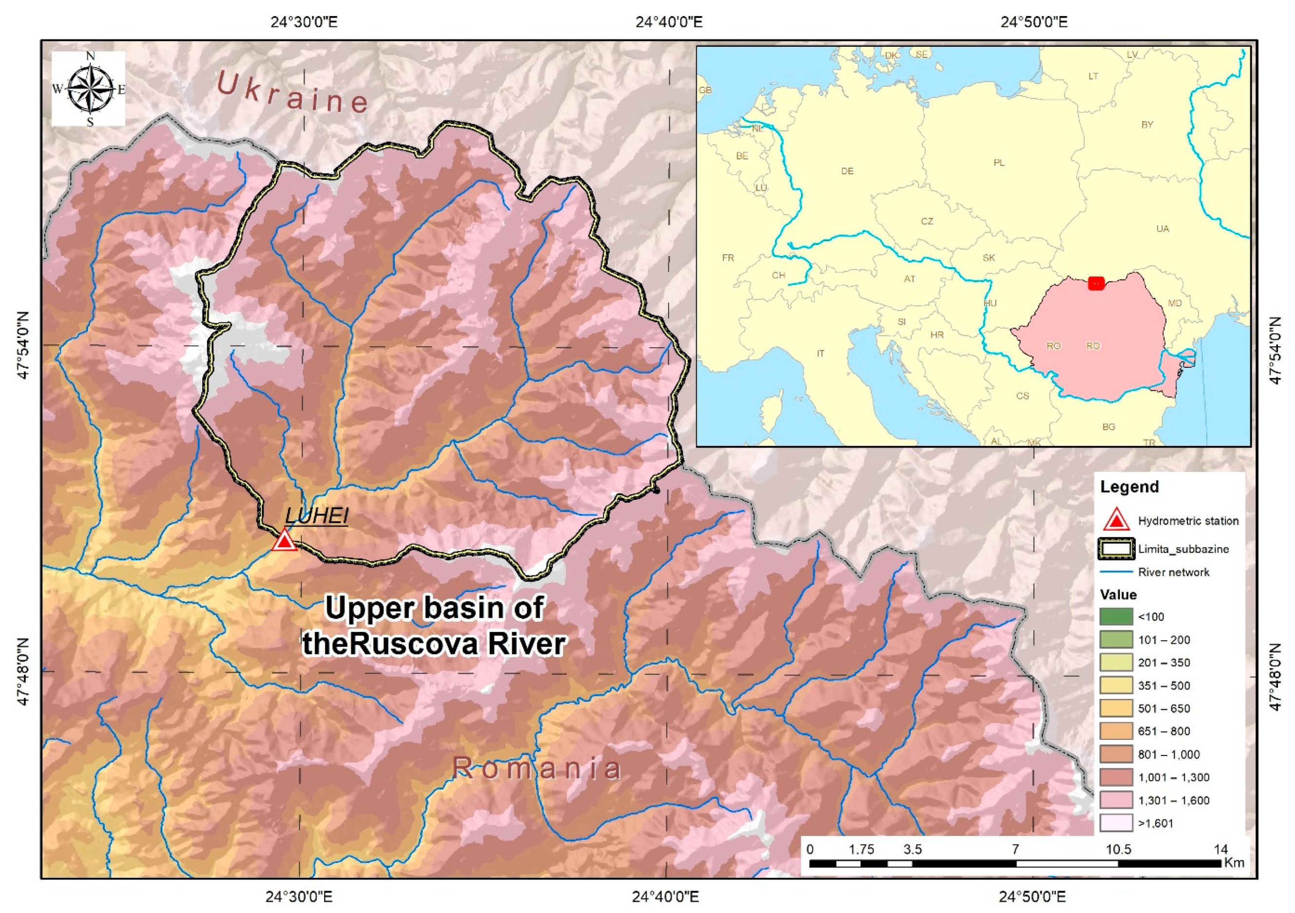
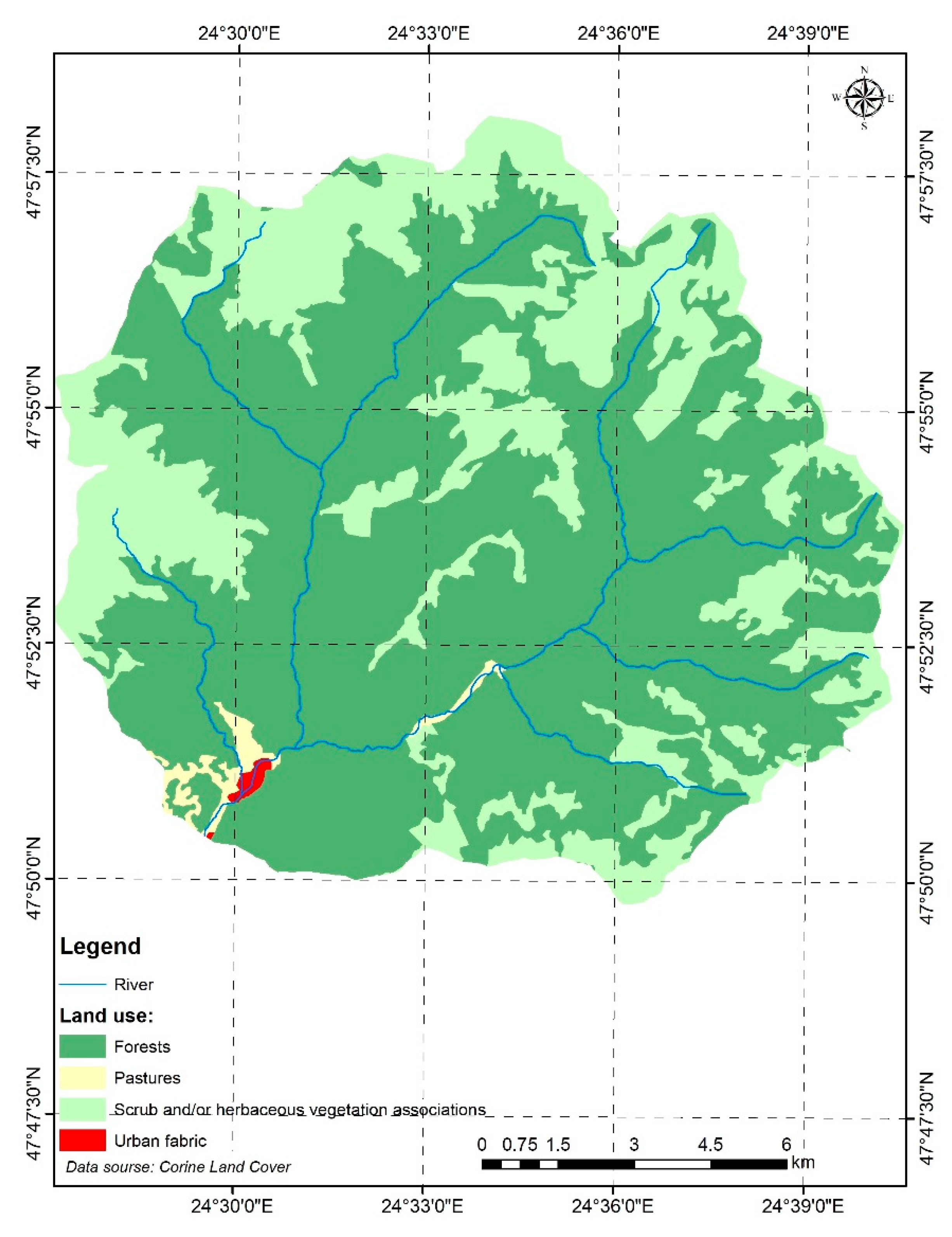
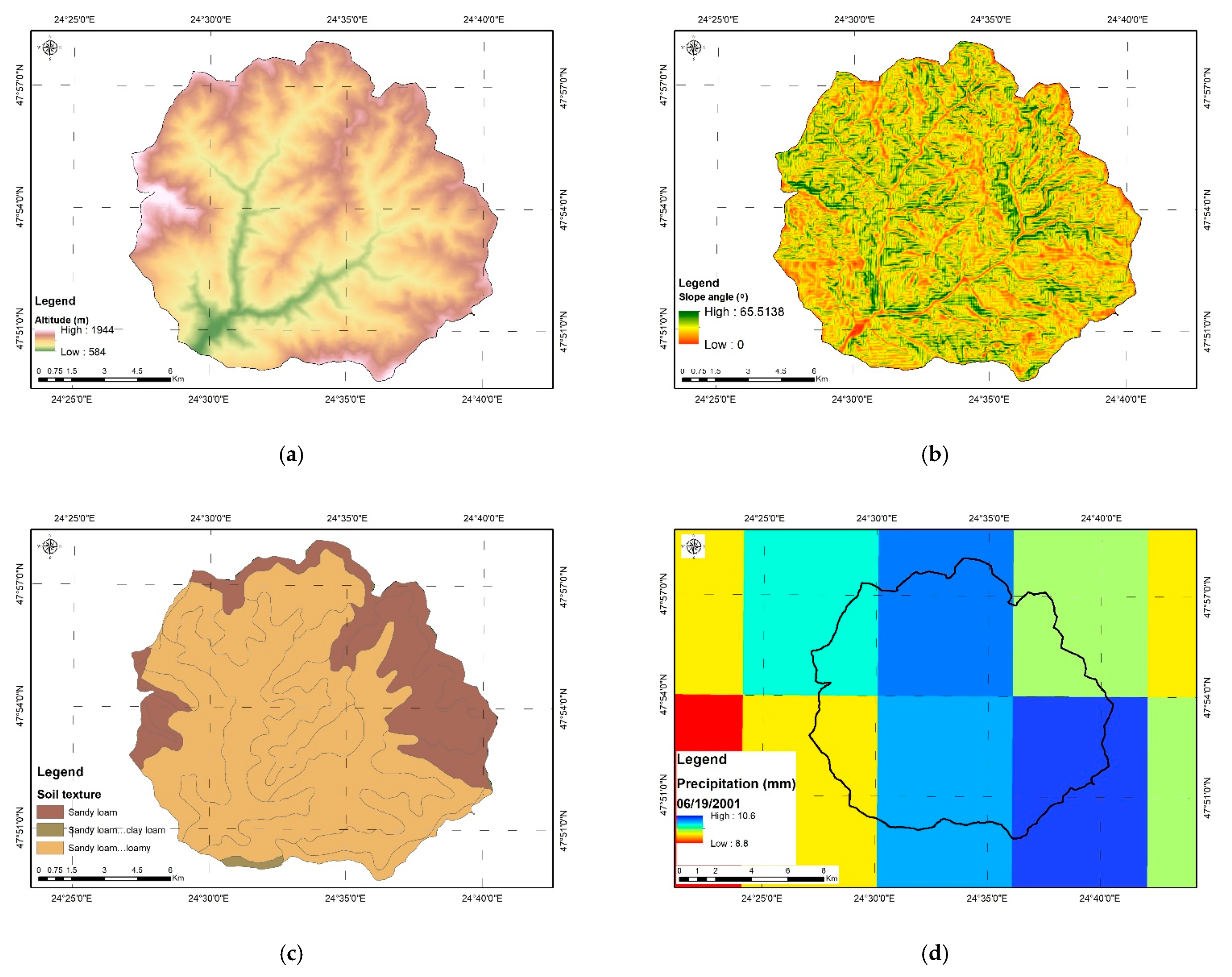
2.1. Study Area

For this study, the upper basin of the Ruscova River (right tributary of the Viseu River) was chosen. This small basin (185.6 km²) is located in northern Romania (47°50′ N and 24°30′ E), close to the border with Ukraine (Figure 1). Over a period of 70 years (1950–2020), the focus region registered a multi-annual average amount of precipitation of 913 mm, and the snow cover lasts, on average, 240 days (from October to May). The mean multi-annual temperature of the region is 3.4 °C.

In the study area, a snow-dominated hydrologic regime is characteristic. In spring, there are high waters dominated by melting snow and high amounts of precipitations; in summer and autumn, waters are generally low due to the global evaporation which is interrupted by floods due to torrential rains. At the end of autumn and in winter, there are also low waters: in autumn due to the lack of precipitation, and in the cold season because a part of the water is retained in the ice formations and because the precipitations are in a solid form.

Concerning the altitude of the basin, the upper basin of the Ruscova River is located between 584 and 1944 m. The topography is characterized by steep slopes (the average slope of the basin is 42.52%).

From the total surface of the upper basin of the Ruscova River, 69% (in the year 2018) is covered by forests (Figure 2). The predominant types of forests are mixed forest, formed by coniferous and broad-leaved forests (26.5%), followed closely by coniferous (25.2%) forests and, with a smaller weight, broad-leaved forests (17.3%). Among the tree species, fir and spruce are dominant, but soft-deciduous mixed forests are present too.

The basic criteria for choosing this river basin were the following:

• The surface of the river basin must be covered as much as possible by forest;
• There are no human settlements or elements of infrastructure that would lead to the permanent reduction in forested areas;
• Afforestation and deforestation actions were detected in the focus area over recent decades.

The upper basin of the Ruscova River is characterized by large areas covered by forests. Over time (especially in the period 1995–2010, in the focus region, more or less legal deforestation has been carried out, or numerous destructions due to natural causes (storms or erosions) have occurred. There were also several campaigns to reforest the area by ROMSILVA (Romania’s National Forest Administration is the Romanian state company in charge of protecting and managing the Romanian public property forests).

Out of the total area of the focus region, 70.1% is covered by acid brown soils. These types of soil are formed in cold and humid climates, which causes the organic matter to be only partially decomposed by microorganisms, and the very slow process leads to an increased acidification of the soil. They are poor in nutrients with a high-permeability texture and are generally covered with forest vegetation. Along with acid brown soils, lithosols (1.3%) and feriiluvial brown soils (podzolic) (28.6%) are present.

2.2. Data Used

2.2.1. Precipitation

Precipitation data were extracted from the daily gridded dataset provided by the European Climate Assessment and Dataset project (EOBS) [25,26]. The EOBS daily gridded database is an ensemble dataset developed at the European level for the period 1950–2020 (updated year by year). The spatial resolution of the grid is 0.1° × 0.1° (~8 km × 8 km). The comparative analysis between the EOBS gridded dataset and the observed values for the NW area of Romania recommended their use for this type of analysis [27].

2.2.2. Runoff Data

For the runoff data, we used one gauging station which is part of the Romanian national network of hydrology and water management: Luhei Hydrometric Station on the Ruscova River (Figure 1), and the data were daily mean discharge values for the entire study period.

2.2.3. Satellite Images

Analysis of the evolution of the forest area was made based on the Landsat Multispectral Scanner (MSS) Surface Reflectance images freely provided by the United States Geological Survey (USGS) for the period 1985–2019 (Landsat 4–8) [28]. All used images are cloud-free.

The analysis of the method’s accuracy was performed based on the orthophoto images provided by the Romanian National Cadastral Agency and Real Estate Advertising service [29].

2.3. Methods

The forest plays a significant role in the soil–water–atmosphere system [30]. Thus, precipitation water partially seeps into the looser soil of the forest, another part is retained by the canopy of trees and subjected to the process of evapotranspiration and perspiration, another amount is consumed by tree roots and transformed into sap and another significant part flows as surface runoff [1,10,30]. Therefore, in the analysis of the influence exerted by the forest on the runoff, the following information and data are needed:

• The amount of precipitation falling in a certain area;
• The evolution of the forest area over a certain period of time (afforestation and deforestation actions) in the focus region;
• The evolution of potential evapotranspiration;
• The amount of water drained (flow) at the closing section of the analyzed basin.

2.3.1. Estimating the Amount of Precipitation

Correct determination of the amount of precipitation is an essential step in this analysis. Using the geographical limits of the basin, all the daily data series contained in the EOBS gridded dataset for the period 1985–2019 were extracted. Then, the extracted values for each grid were mediated to determine the average amount of precipitation falling in the watershed.

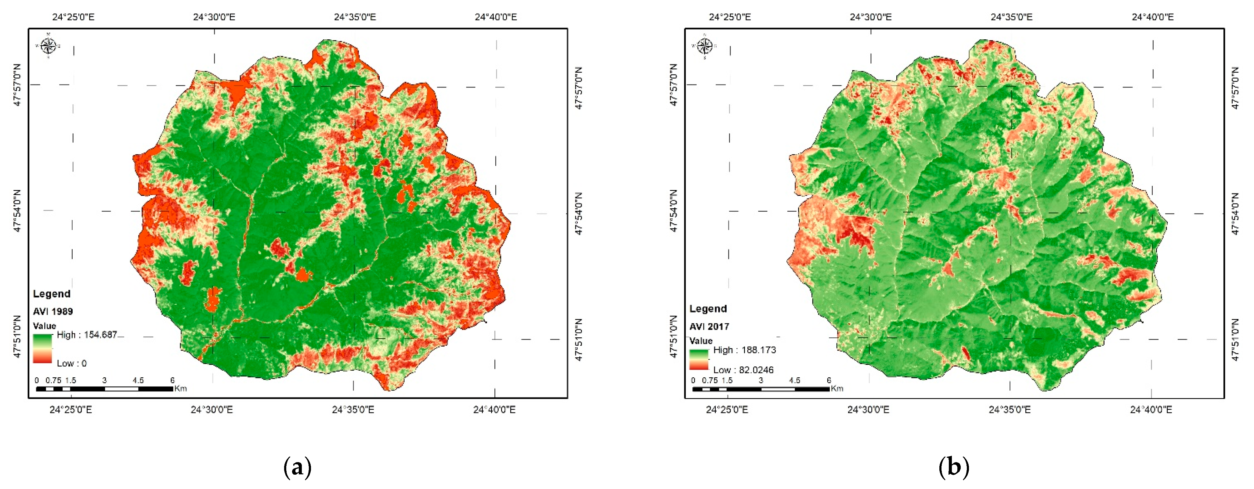
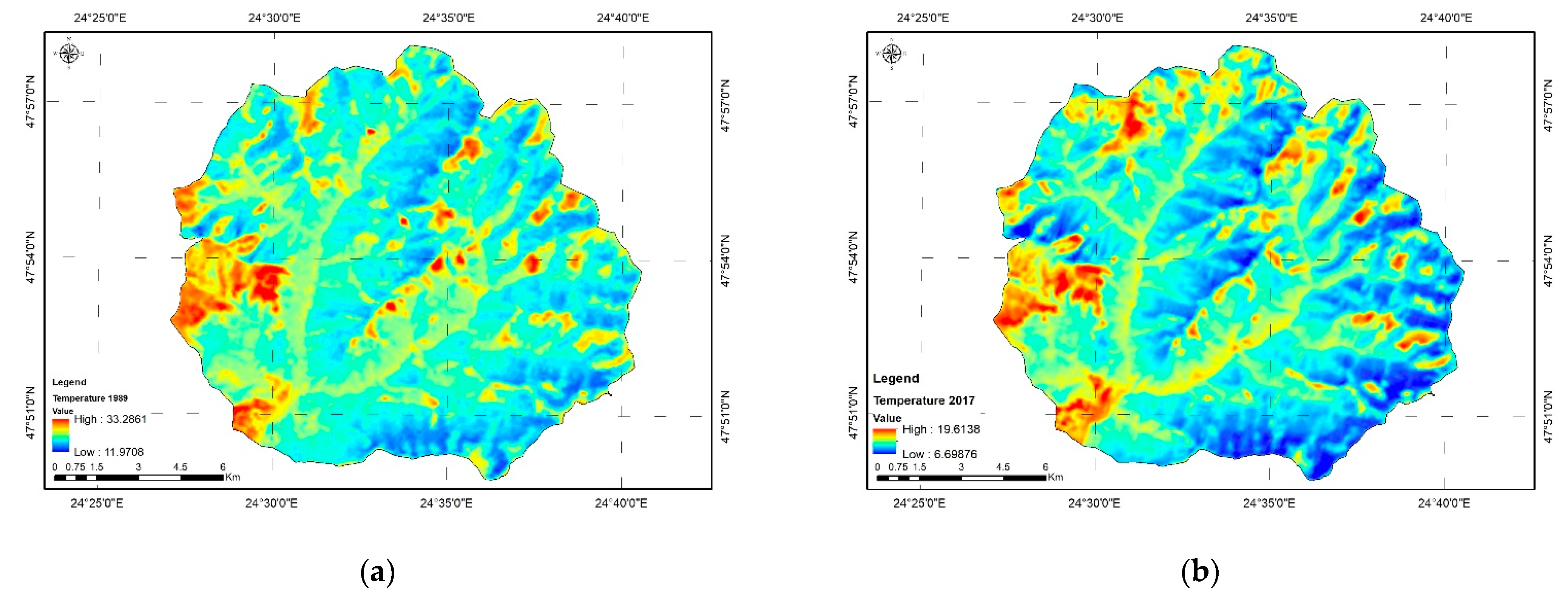
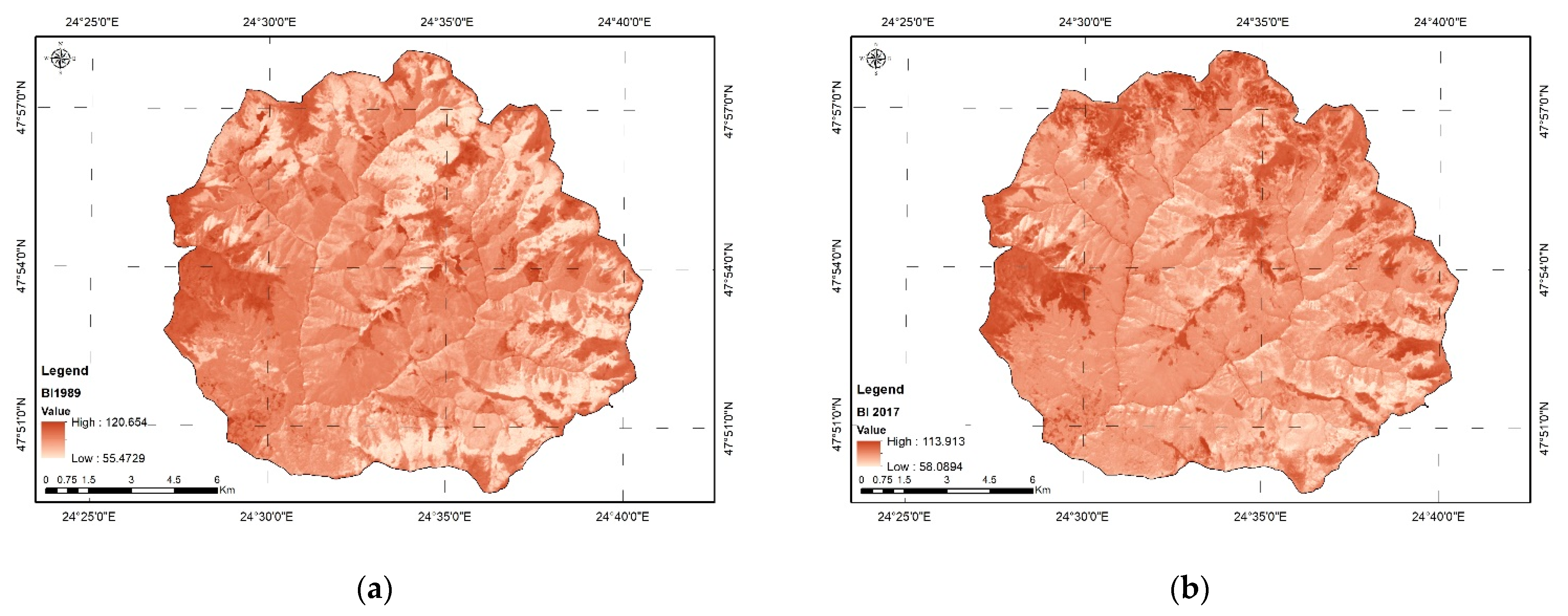
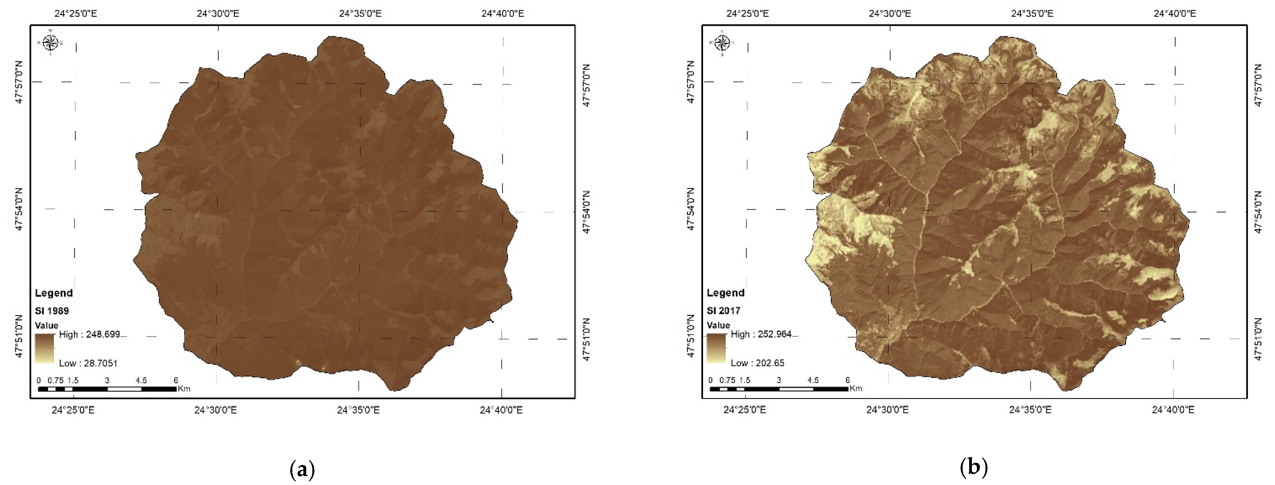
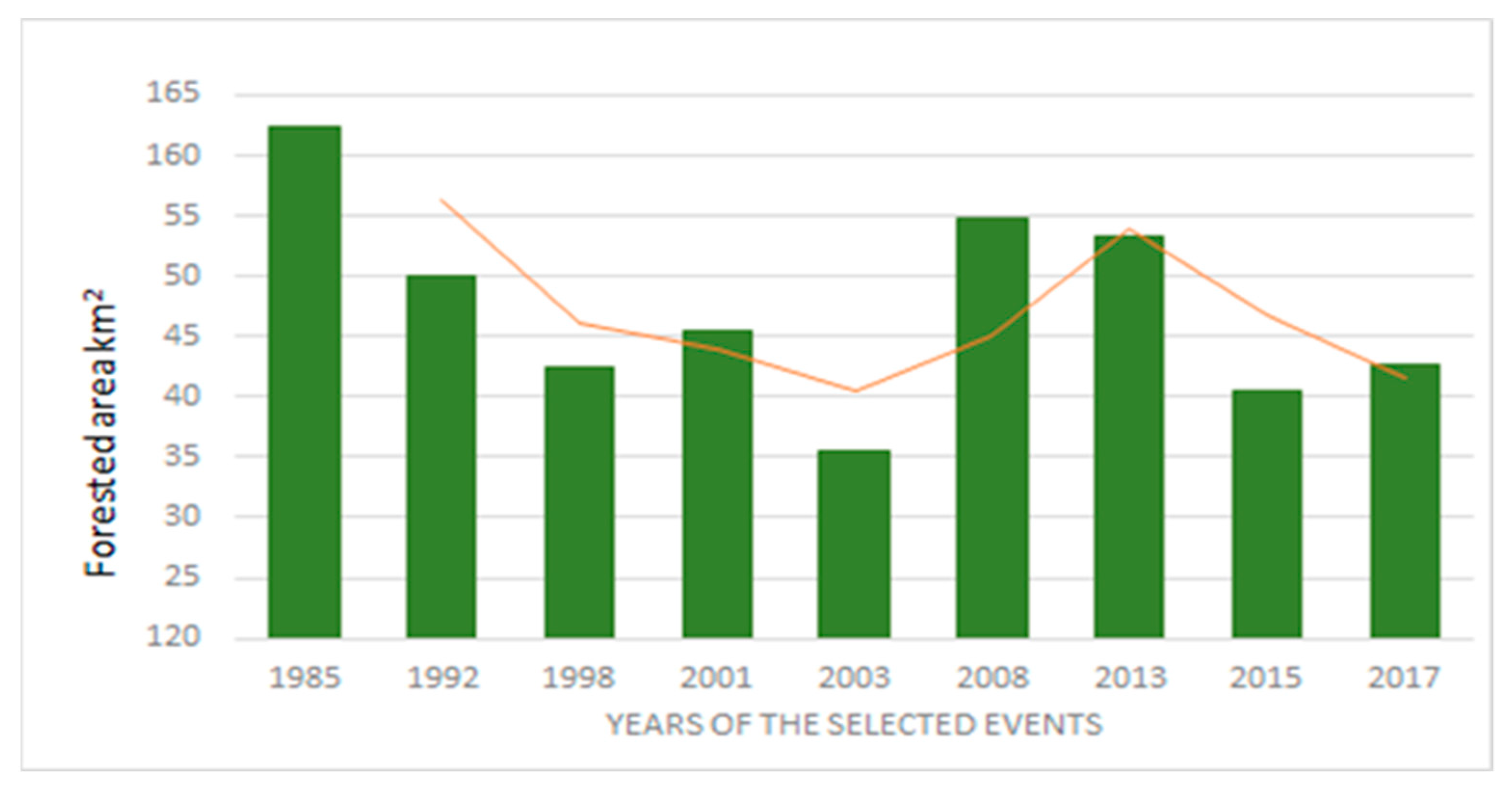
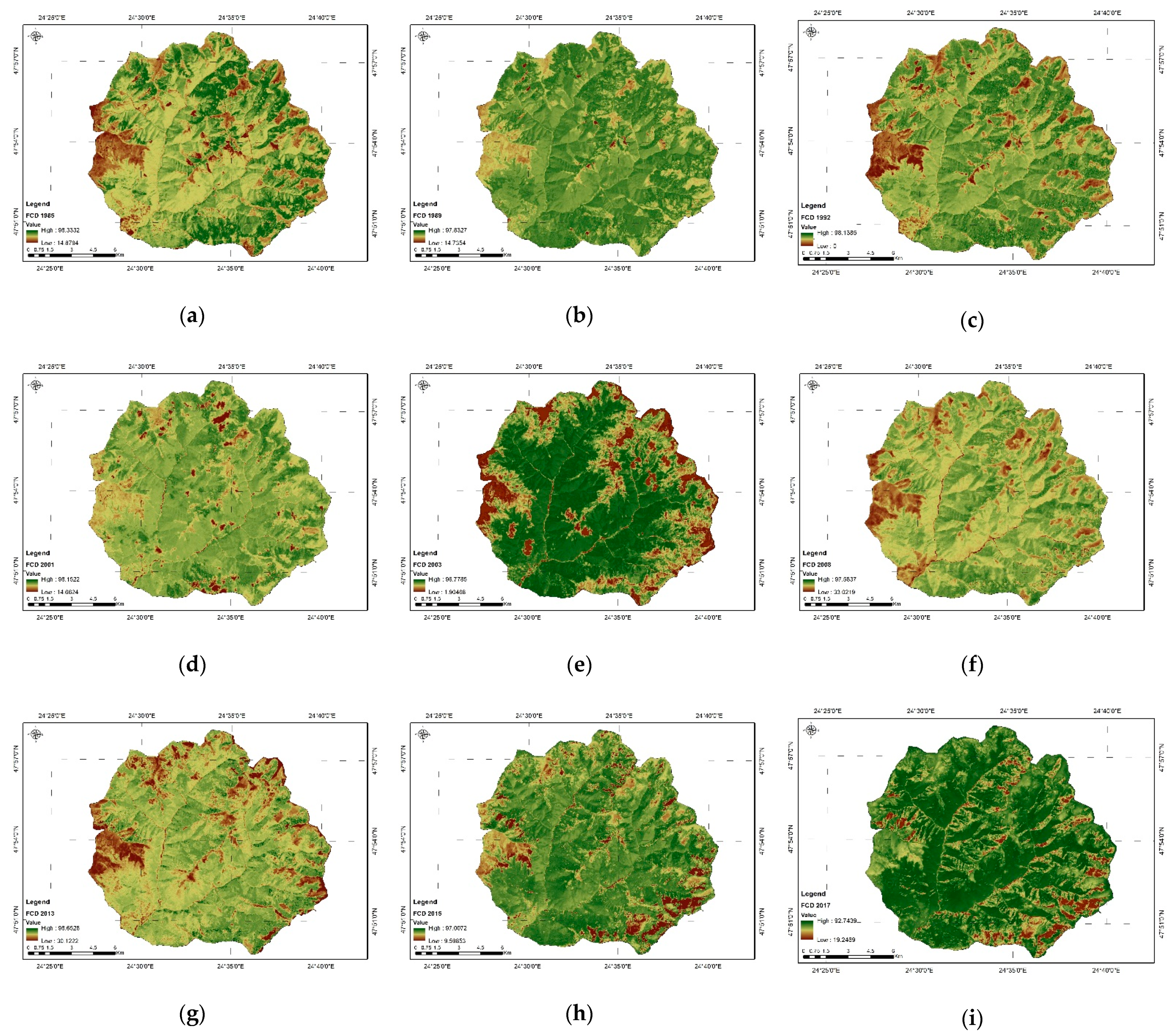
2.3.2. Evolution of Forest Area and Density

In the analyzed area, for the period after 1985, no first-hand reliable information was found regarding the evolution of forested areas. To follow the evolution of the afforested surfaces in the study area, several vegetation indices were extracted and analyzed from the Landsat images for the period 1985–2019. The following issues were taken into account:

• The image collection period should be in the interval between the end of May and the start of October so that the phenophase of the forest is somewhat similar, fully developed canopy;
• The analyzed surfaces should not be covered by clouds.

Since the research area is located in a mountain region characterized by high cloudiness, it was quite difficult to identify images without significant cloud cover for each year after 1985.

Table 1. Specification of Landsat data used in study.

Sensor	Data	PATH/ROW	Scene Center Time
Landsat 5 TM	14 August 1985	184/027	08:38:11.6210310Z
Landsat 5 TM	25 September 1992	185/027	08:36:35.8650620Z
Landsat 5 TM	10 September 1998	185/027	08:53:24.1940000Z
Landsat 5 TM	16 July 2001	185/027	08:55:05.7030940Z
Landsat 7 ETM	27 May 2003	185/027	09:03:24.1067109Z
Landsat 5 TM	13 August 2008	185/027	08:54:29.1940500Z
Landsat 8 OLI_TIRS	5 October 2013	185/027	09:16:35.6672900Z
Landsat 8 OLI_TIRS	8 August 2015	185/027	09:14:20.7774850Z
Landsat 8 OLI_TIRS	14 September 2017	185/027	09:14:48.6049790Z
Landsat 8 OLI_TIRS	19 August 2019	185/027	09:14:51.5805550Z

shows the data and characteristics of satellite images considered in this analysis; all images have a 30 m spatial resolution and are from the T1 collection category.

Landsat Surface Reflectance images provided by the U.S. Geological Survey were used [28]. These images measure the fraction of incoming solar radiation reflected from Earth’s surface to the Landsat sensor, for Landsat missions 5, 7 and 8.

All images are converted within an 8-bit range.

To choose the best method, we tested several vegetation indices (VI) obtained based on the analysis of the spectral bands of Landsat satellite images: leaf area index (LAI), normalized difference vegetation index (NDVI), enhanced vegetation index (EVI), a soil-adjusted vegetation index (SAVI), forest canopy density (FCD). In this evaluation, we used predefined indices in different programs, such as the Raster Function module of ArcGIS PRO software (produced by ESRI US) for NDVI and LAI indices, or we analyzed the satellite images using the software function Sentinel Application Platform (SNAP) produced by the European Space Agency (ESA) for SAVI and EVI indices.

The best results were obtained using the method proposed in [31,32,33] for the determination of the FCD index. It is defined as the proportion of coverage of the forest floor by the vertical projection of the peaks of trees, and it is also known as crown coverage or canopy coverage [34,35]. The FCD index is achieved by composing four other indices: advanced vegetation index (AVI), canopy shadow index (SI), bare soil index (BI), thermal index (TI).

Using the Model Builder implemented in the ArcGIS desktop program, a workflow was implemented (see Supplementary Material Figure S1) to obtain the FCD map, as described in Figure 3.

Image Normalization. The first step in obtaining the four already mentioned indicators was the normalization of the spectral bands. This stage involves the elimination of distortions caused by the angle of the Sun with the vertical of the place at the zenith, the average Earth–Sun distance when taking the image, atmospheric conditions, etc. [36].

The Landsat TM bands (except for band 6) were normalized using linear transformation (Equations (1)–(3)):

$$\mathrm{A}=\frac{\left(Y1+Y2\right)}{\left(X1-X2\right)}=\frac{20-220}{\left(M-2S\right)-\left(M+2S\right)}=\frac{50}{S}$$

(1)

$$B=AX1+Y1$$

(2)

$$Y=-AX+B$$

(3)

where $X1=M-2S$; $X2=M+2S$; $Y1=20$; $Y2=220$; M—mean; S—standard deviation; X—original data; and Y—normalization data.

Obtaining the Four Vegetation Indices.

According to the methodology proposed by Rikimaru [31,32], we employed the following vegetation indices, derived from satellite images.

Advanced Vegetation Index (AVI). This method uses the combination of red and near-infrared (NIR) bands. By raising the power, the spectral signature of chlorophyll is amplified. This way, the index is able to capture the factors and type of vegetation (it is able to identify vegetation inversions, but especially the anthropogenic influence of reforestation). Equation (4) shows how to obtain this indicator:

$$\begin{array}{c}AVI={\left[\left(B4+1\right)\times \left(256-B3\right)\times \left(B4-B3\right)\right]}^{1/2}\\ AVI=0 If B4<B3 \mathrm{after} \mathrm{normalization}\end{array}$$

(4)

where:

B4—near-infrared band;

B3—red band.

Results of the analysis performed for the years 1989 (a) and 2017 (b) (Landsat 5 and 8) are shown in Figure 4.

Bare Soil Index (BI). Adding an index to identify bare soil surfaces, in combination with vegetation indices, results in a stronger contrast in the analysis [31,32,33]. The basic logic of this approach is to build on the high reciprocity between the state of the bare soil and the state of vegetation. By combining vegetation and bare soil indices in the analysis, one can assess the state of forests on a continuum ranging from high vegetation conditions to exposed soil conditions.

BI (Figure 5) was calculated by using Equation (5):

$$BI=\frac{\left(B5+B3\right)-\left(B4+B1\right)}{\left(B5+B3\right)+\left(B4+B1\right)}\times 100+100$$

(5)

where:

B5—shortwave infrared band;

B1—blue band.

Shadow Index (SI). The use of this index highlights the three-dimensional characteristics of the forest by placing the focus on the shaded areas of the forest canopy. It is based on the low brightness of the visible bands. Through this process, younger tree structures can be identified [31,32,33]. These structures usually have a lower brightness than more mature trees. At the same time, this index allows the delineation of the surfaces covered by bushes and shrubs from the surfaces with trees.

The shadow index is calculated using Equation (6):

$$SI=\sqrt{\left(256-B1\right)\times \left(256-B2\right)\times \left(256-B3\right)}$$

(6)

where:

B2—green band.

The SI value is directly proportional to the height of the canopy and the density of the forest (Figure 6).

Thermal Index (TI). This index was developed considering that bare surfaces (without vegetation) have a higher temperature at ground level than shaded surfaces in areas covered by forests [33]. This indicator allows distinguishing between the shaded slopes with forests and the shaded slopes without forests.

The first step in obtaining the brightness temperature is to convert the reflectance values into radiant values by using relation 7:

$$L=\frac{L_{MAX}-L_{MIN}}{255}\times DN+L_{MIN}$$

(7)

where:

L—spectral radiance at the pixel level (meter squared * ster* μm):

For Landsat missions 5 and 7, L_MAX = 15.303 (spectral radiance of DN value 255), and L_MIN = 1.238 (spectral radiance of DN value 1); for Landsat 8, L_MAX = 22.00180 (spectral radiance of DN value 65,535), and L_MIN = 0.10033 (spectral radiance of DN value 1);

DN—digital number or spectral value of the pixel.

By employing the spectral radiance and some calibration coefficients (K1, K2), the temperature at ground level is derived, as presented in Equation (8):

$$T=K2/(\ln \left(\frac{K1}{L}+1\right))/275$$

(8)

where:

T—brightness temperature (°C).

For Landsat missions 5 and 7, K1 = 666.09 watts (m2/sr/µm), and K2 = 1282.71 K; for Landsat 8, K1 = 774.8853 watts (m2/sr/µm), and K2 = 1321.0789 K.

In Figure 7, images with the TI for the years 1989 (a) and 2017 (b) are presented.

Combining Indices to Achieve the FCD Model.

The composition of the FCD model implies the derivation from the initially obtained indices of two other indicators: the vegetation density (VD) and the scaled shadow index (SSI).

VD is obtained by synthesizing the AVI and BI indices by the principal component analysis method [31,32,33]. Next, each pixel value is divided by the maximum value and multiplied by 100 to obtain the percentage value.

The SI index is an index whose value depends on the low irradiant area of each visible band. The use of the SI indicator to determine the SSI may present false information due to the possibility of delimiting including the shaded slopes. As bare soils have a higher temperature than the shady ones (due to their higher capacity to absorb solar radiation), the SI was combined with the TI index. Thus, the possible errors generated by the exposure of the slopes are avoided [31,32,33]. In the next step, this indicator was transformed by relating each pixel to the absolute maximum value. The SSI value is scaled from 0 to 100%: the value of SSI 100 corresponds to a forest with the highest shadow value, whereas the value of 0 indicates a forest with the lowest shadow value. Thus, in areas where the SSI is 100, forest is present.

FCD. This step involves combining the VD and SSI (Equation (9)) [31,32,33]. As the values of the two parameters represent the percentage of values, the FDC ranges from 0 to 100:

$$FCD=\sqrt{\left(VD\times SSI+1\right)-1}$$

(9)

Figure 8 shows the images with the FCD for 1989 (a) and 2017 (b).

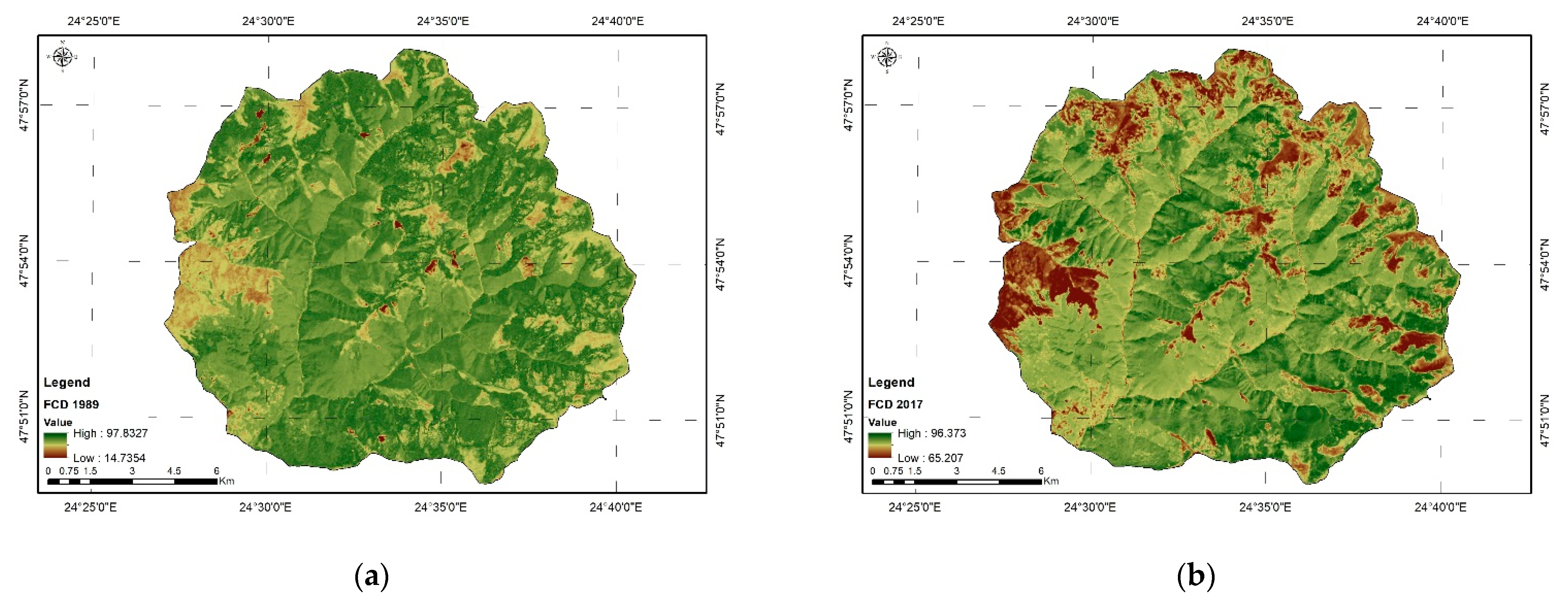
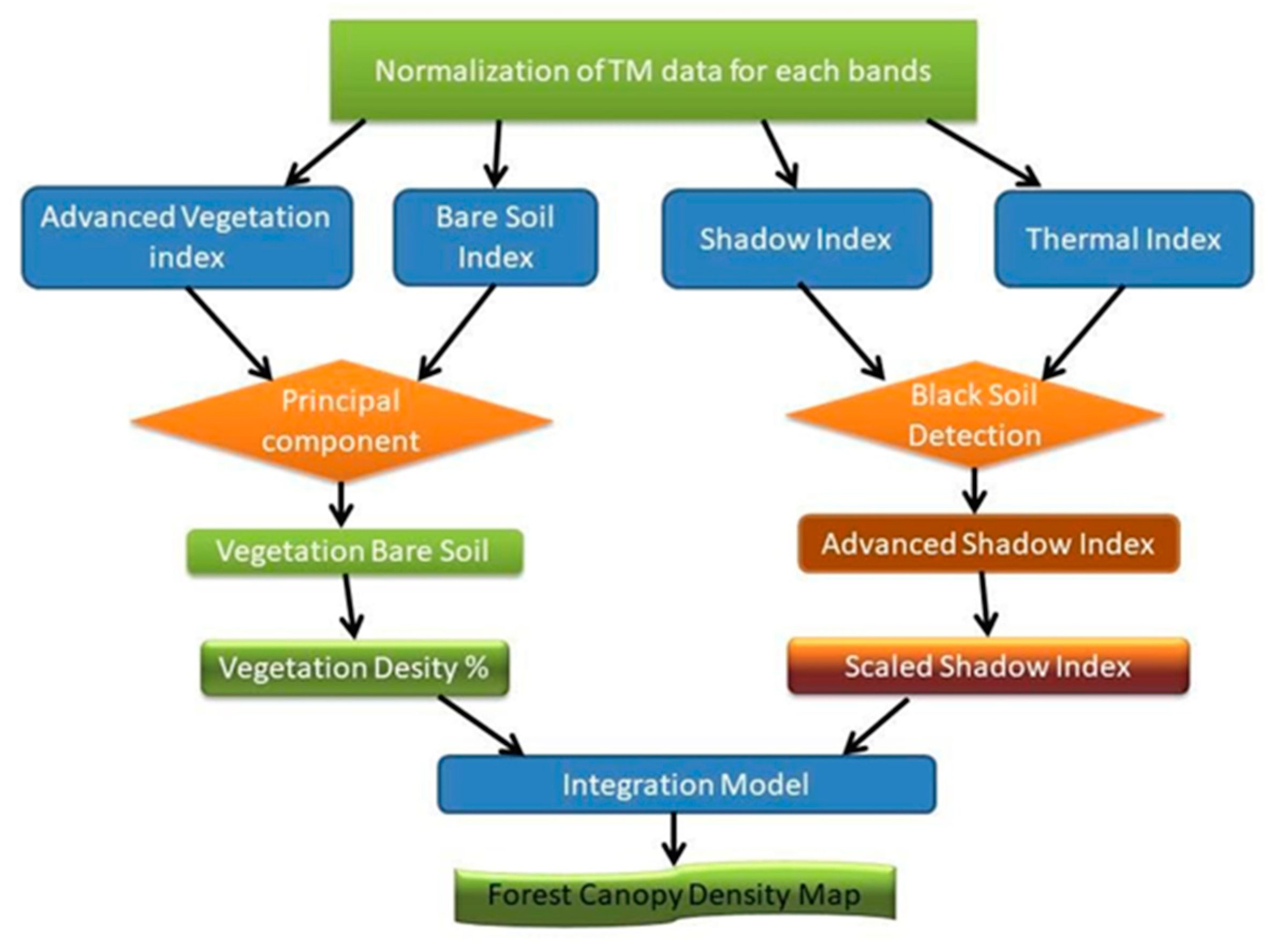
2.3.3. Evaluation of the Method for Determining the FCD Index

For evaluating the method, we used the kappa coefficient (κ), which is employed to measure the accuracy of a method by evaluating the actual values, derived from observations and the estimated ones, determined by calculation [37].

To perform this analysis, we created 20 random points that we intersected with the FCD layers made for each analyzed year. For intersections with forest areas, they were quantified as 1; for intersections with pasture areas, we used 0. The comparison of these estimated values with the observed values was conducted by comparing them with aerial photographs from 2018, where the same scores of 1 and 0 were given.

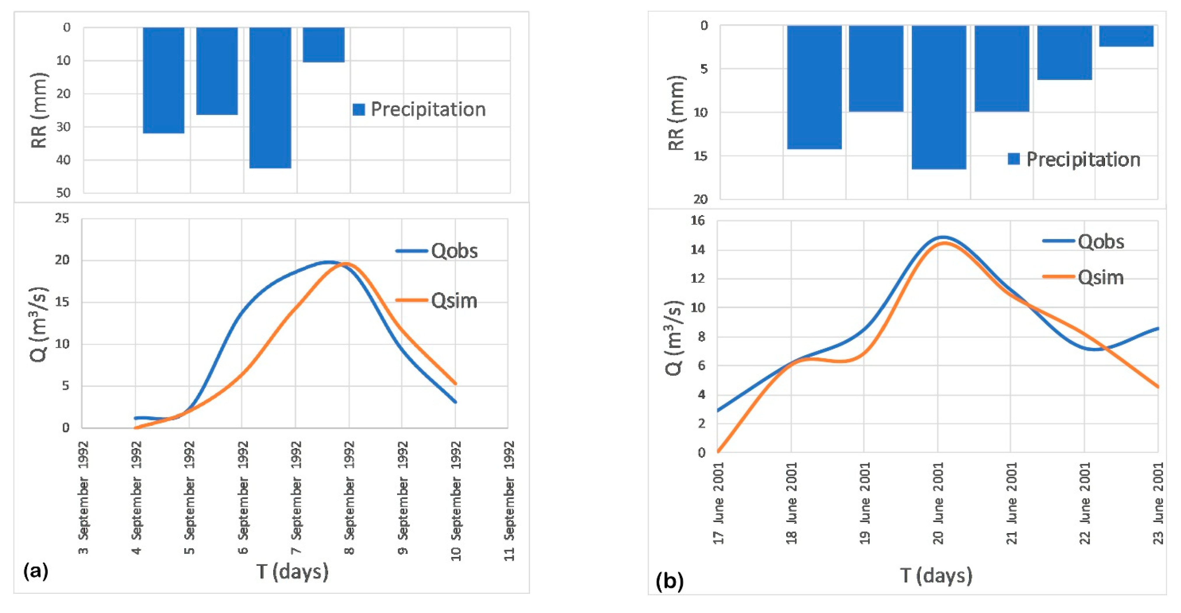
2.4. Analysis of Precipitation Values and Flow Hydrographs Related to the Evolution of Forest Surfaces

The entire amount of precipitation that falls in a region does not reach the hydrographic network. Part of this amount is returned to the atmosphere by evapotranspiration, another part is absorbed by vegetation at the interception level and yet another part infiltrates and forms underground runoff and/or hypodermic runoff.

The comparative analysis of the discharge values with the surface covered by forest or a comparative analysis between runoff coefficients with the forest surface values can give us an image of the influence of the forest surfaces on the river discharge in the analyzed area. However, this comparative analysis is not sufficient to determine the impact that the forest has on the runoff. For such an analysis, a hydrological model able to simulate hydrological processes is required. One of the setting parameters of the model should be the vegetation, or an index derived from it.

For this study, we used the well-known unit hydrograph method (UHM) from the Mike Hydro River modeling system produced by DHI [38,39].

This type of model cannot simulate events in which snow influences the flow of the watercourse. That is why this model is not recommended to be used for those events in which snow or melting snow influences the runoff. In the UHM module, the excess rain is calculated assuming that the losses to infiltration can be described by the SCS generalized CN (Soil Conservation Service curve number) method [39], which is a simple and efficient method for determining the approximate amount of runoff from a rainfall event in a particular area. The curve number is a dimensionless index, which can take values from 0 to 100. It is based on both land use and the hydrologic soil group and reflects the potential to generate water runoff on different surfaces.

2.5. Hydrologic Model

2.5.1. The Basin Model

The main thematic map layers used in setting up the model are presented in Figure 9. For the digital elevation model (DEM) (Figure 9a), we used the Shuttle Radar Topography Mission (SRTM) freely downloaded from the U.S. Geological Survey website, with a spatial resolution of 30 m.

By processing the DEM using the spatial analysis tools of the ArcGIS Pro software (ESRI, US), a series of parameters required by the model was extracted: slope angle (Figure 9b), flow direction, flow length, sub-basin delineation.

The data source referring to the soil texture, used in the model to determine the value of the CN index (Figure 9c), is the National Research-Development Institute for Pedology, Agrochemistry and Environmental Protection Bucharest (ICPA). The spatial resolution of the soil map is 1:25,000.

Based on the river basin catchment area, we extracted the related precipitation data series. The spatial representation of the extracted values is points located in the center of each grid cell. Further on, based on the grid pixel centers, Thiessen polygons were derived, and their overlap in the basin area allowed us to calculate a weighted average of precipitation values for the considered area (Figure 9d).

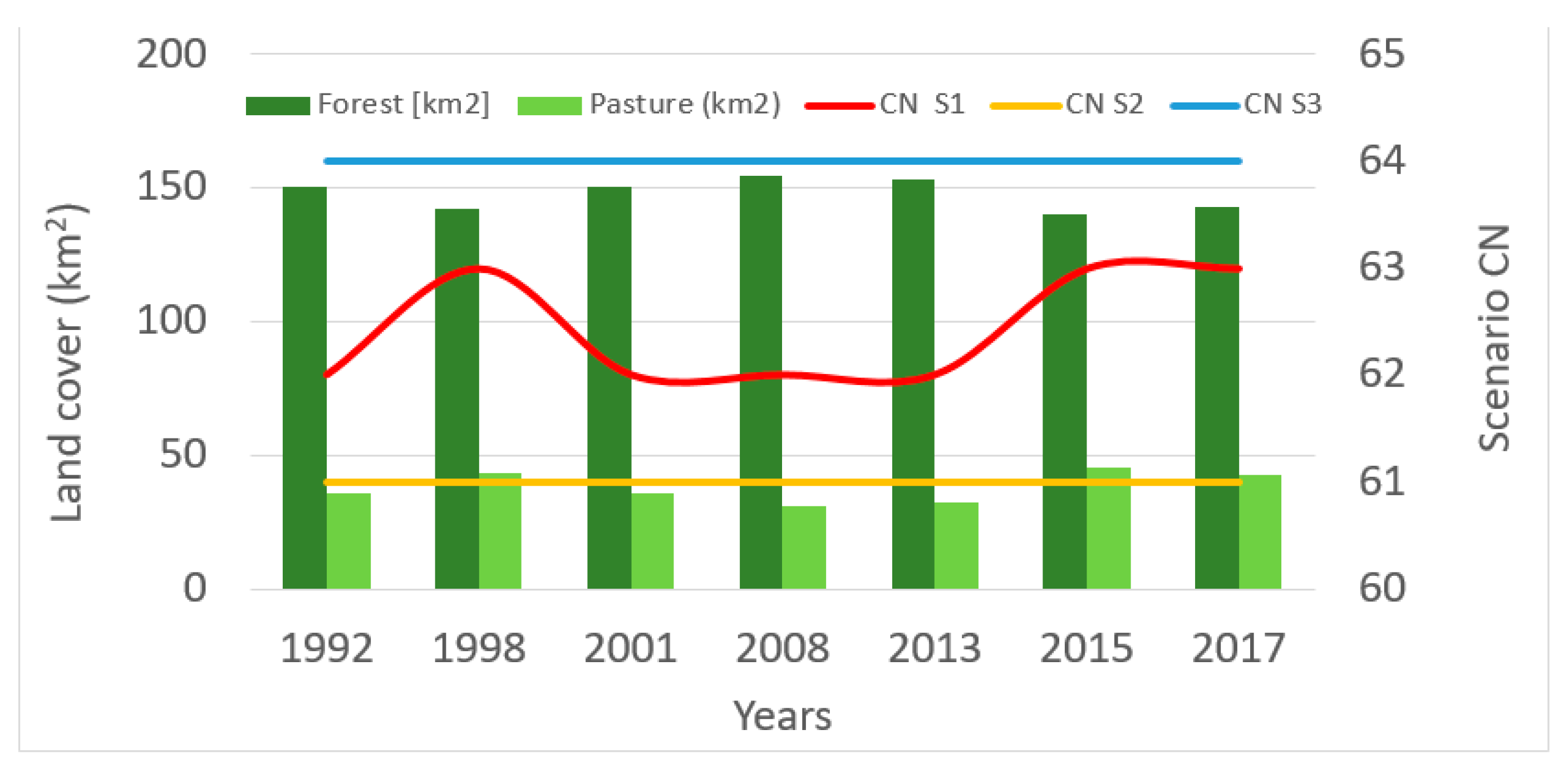
2.5.2. Soil Conservation Service (SCS) Generalized (CN) Loss Method

As mentioned above, the CN is based on the area’s hydrologic soil group, the type of land use and the hydrologic condition. The U.S. Soil Conservation Service developed this method for computing losses from storm rainfall in 1972 [37,38,39].

The general equation for the SCS CN method is as in Equation (10):

$$Q=\frac{{\left(P-I_a\right)}^2}{\left(P-I_a\right)+S}$$

(10)

where:

Q—runoff(m³/s);

P—precipitation (mm);

S—potential maximum retention after runoff begins;

I_a—user-defined initial loss (mm).

According to the DHI Mike 11 Reference Manual [38,39], an empirical relation was developed after testing several small experimental watersheds (Equation (11)).

I_a = 0.2 × S

(11)

The potential maximum retention S is calculated from a dimensionless CN using the empirical formula derived by SCS based on rainfall runoff analyses of a large number of catchments. The value of S can be calculated with the formula (Equation (12))

$$S=\frac{25400}{CN}-254$$

(12)

In this analysis, we used the SCS generalized method. The main difference from the SCS CN method is that the SCS generalized method does not make use of the concept of an antecedent moisture content (AMC) but applies a storage initial abstraction depth [38,39,40].

Establishing the Soil Hydrological Groups

As presented in Equation (11), the maximum retention potential is based on the CN, which is determined based on the hydrological group of soils and land use at the level of the river basin. From this point of view, the soils were classified into 4 hydrological groups (A, B, C and D), depending on the water infiltration rate. Chendes [41] adapted the soil hydrological groups classification to the Romanian soil classification system. Here, we used the same approach. The classification is based on the texture of the soil, assessing the percentage of sand, silt and clay in each type of soil, which provides a characteristic from permeable to impermeable soil or from light (sandy) to heavy soil (clays) (see Supplementary Material Table S1).

The analyzed area does not have a great diversity of soil textures. Only three types of textures were identified: sandy-loam–loamy (75.7%), sandy-loam (23.8%) and sandy-loam–clay-loam (0.5%). The high percentage of the sandy–loamy soil texture is due to the fact that most of the focus region is forest land, and the main species are coniferous (Figure 9c).

CN Calculation

Based on the soil texture and land use categories, the following CN values were determined (

Table 2. The CN values of land use types and hydrologic soil groups used in the present study.

Nr.crt	Land Use	Hydrologic Soil Group
		A	B	C	D
1	Discontinuous urban fabric	-	89	-	-
2	Pastures	-	69	-	-
3	Broad-leaved forest	-	66	-	-
4	Coniferous forest	34	60	73	-
5	Mixed forest	38	62	75	-
6	Natural grasslands	49	69	79	-
7	Moors and heathland	49	69	-	-
8	Transitional woodland-shrub	45	60	-	-

CN values adjusted for Romania after Chendes [41].

):

In order to determine a single value of the CN index, a weighted average value was computed using the corresponding area for every land use type (Equation (13)):

$$\overline{x}=\frac{{{\displaystyle \sum }}_1^{n}ci x_i}{A}$$

(13)

where:

($\overline{x}$)—area weighted average CN;

c_i—certain land use area;

x_i—the values x₁, x₂…x_n represent the CN values from the original reference table [39,41];

A—total area of the river basin.

The above procedure is necessary to measure the contribution of the land use type (in our case, forested areas) to the runoff. In essence, by modifying the surface area of the forest and the pastures, we automatically obtain a different CN, which influences the simulation of the runoff during a certain event.

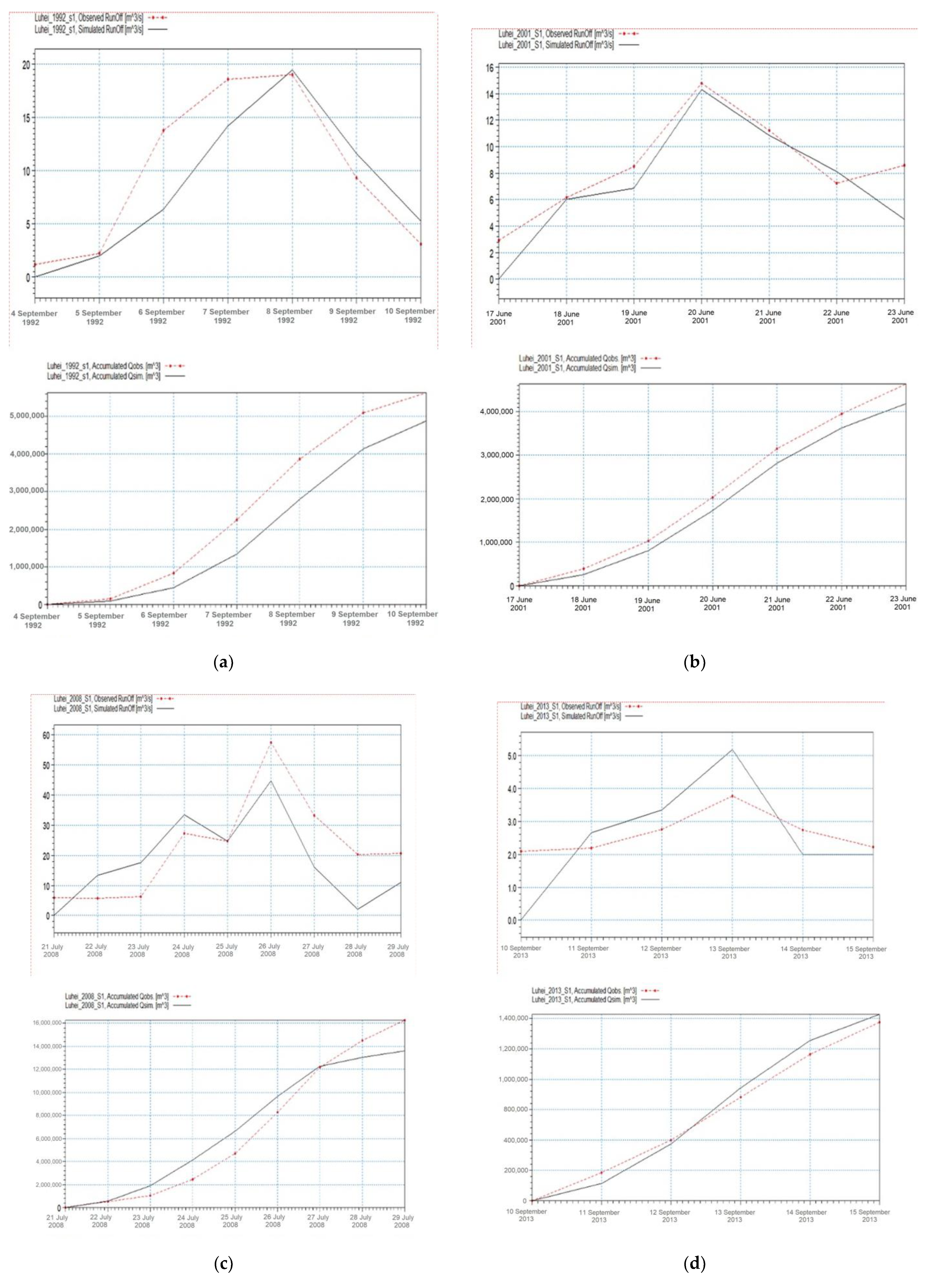
2.5.3. Model Calibration and Event Isolation

UHM is used to estimate the runoff of a single storm event using the well-known unit hydrograph technique. The models divide storm rainfall into excess rainfall (or runoff) and water loss (or infiltration). From a conceptual point of view, this model represents the average response of a unitary surface of the hydrographic basin to the impulse generated by the excess of precipitations. Therefore, for each calculation time step, the model determines the response of the basin to excess rainfall, as generated by the loss model during the time step, and cumulates this response with the flow values formed in the previous time steps [38].

The following parameters were used for model calibration: lag time, hydraulic length, slope of the catchment, baseflow, catchment area and the CN.

Most of these parameters (except for the CN value) were extracted from the DEM, using the spatial analysis tools of the ArcGIS Pro program. The values used to calibrate the model are presented in

Table 3. Values of parameters used to calibrate the model.

Hydraulic Length (km)	Slope (%)	Baseflow (m3/s)	Catchment Area km2
6.124 km	42.5	2	185.656

. The CN values are variable values depending on the land use area obtained for each year. Its values will be mentioned in the Results section.

The lag time can either be specified directly or may be calculated from catchment characteristics using the standard SCS formula as in (Equation (14)) [39]:

$$t_1={\left(L\times 3.28\times {10}^3\right)}^{0.8}\times {\left(\frac{1000}{CN-9}\right)}^{0.7}/\left(1900\times Y^{0.5}\right)$$

(14)

where:

t_l—lag time in hours;

L—hydraulic length of the catchment (km);

CN—SCS curve number;

Y—average catchment slope (%).

For each analyzed year, an event was isolated to show the evolution of runoff in relation to the precipitation (Figure 10).

The average altitude of the basin and its location favor a long snow cover duration, usually from October to May, but sometimes it extends even into June. The high peak flow of March–April is well above the value of the simulated flow, due to the large amount of snow accumulated during the winter and which begins to melt in April. The situation is somewhat opposite starting from autumn, when the simulated flow values are higher than the observed ones. This situation may be explained by the large amount of precipitation falling and accumulated as a snow layer in the high mountains. The climatic parameter temperature plays an extremely important role in this case; therefore, the model cannot correctly simulate the events that took place during the winter season. Under these circumstances, for model calibration, we selected events only from the warm season (June to September) when the influence of snow melting and deposition is absent.

A difference can be observed between the simulated and the observed values (Figure 10). The causes can be multiple, but the most important seem to be the uncertainties regarding the spatial and temporal variation in the precipitation value, as well as the initial humidity state of the basin; further, the structure of the model can be suspected as a cause, which is too simple. The generalized SCS model used is the only model that captures the influence of vegetation on runoff, using only two parameters for calibration (lag time, CN).

The daily precipitation value contained in the gridded dataset does not allow the detailed capture of the rainfall–runoff response. Although the shape of the simulated discharge hydrograph does not precisely follow the observed one, the overall accuracy of the amplitude and phase of the discharge hydrograph fall under the accepted and recommended thresholds, which confirms the reliability of the model for testing the proposed methodology. The main purpose of this analysis is to calculate the influence of the forested area on the runoff and not a rigorous analysis of the precipitation–runoff phenomenon.

In choosing the events under analysis, we did not necessarily take into account certain characteristics of the phenomenon to look for each year (amount of precipitation, similar duration, etc.) because the pre-event moisture conditions are different from case to case (e.g., the moisture condition prior to the occurrence of the rain event with a direct influence on soil permeability, air temperature, wind speed, etc.). Thus, the events themselves cannot be compared among them in terms of total rainfall amount over a period of time. What we followed in choosing the events was to identify events in which the simulated values are as close as possible to those observed.

2.5.4. Simulated Land Use Change Scenarios

In order to evaluate and understand the influence of reforestation and deforestation actions, it is necessary, first of all, to observe the effects that this change in land use has on the discharge values over time. As the precipitation amount is not the same each year, it is quite difficult to take a reference situation only based on precipitation values and forested areas (identifying two years with similar land use values and observing whether the discharge values are similar). However, because the volume of precipitation events is different, the runoff response or the volume of drained water is expected to be different.

We appreciate that the best method is to take into consideration three scenarios: scenario 1 (S1) is the initial one and by which we calibrate the model for each year event; scenario 2 (S2) assumes the hypothesis that the forested area is at the maximum potential area calculated by the FCD index method (the forested area determined in 1986 was 162 km²); scenario 3 (S3), opposite to S2, refers to the minimum area calculated based on the FCD index and corresponds to that identified for the year 2003 (135 km²) (Figure 11).

3. Results

3.1. Delimitation of Forest-Covered Areas Using the FCD Index

The values of the FCD index for the analyzed years are presented in detail in Figure 12.

Evaluation of the Method for Determining the FCD Index

Analyzing

Table 4. Confusion matrix.

Year	Forest	Non-Forest	Forest	Total	User’s Accuracy	Kappa Coefficient
1985	Non-Forest	2	6	8	0.65	0.186
	Forest	1	11	12
	Total	3	17	13
	Producer’s Accuracy	66.67
1992	Non-Forest	4	4	8	0.75	0.444
	Forest	1	11	12
	Total	5	15	15
	Producer’s Accuracy	80.00
1998	Non-Forest	4	4	8	0.75	0.444
	Forest	1	11	12
	Total	5	15	15
	Producer’s Accuracy	80.00
2001	Non-Forest	3	5	8	0.70	0.400
	Forest	1	11	12
	Total	4	16	14
	Producer’s Accuracy	75.00
2003	Non-Forest	6	2	8	0.75	0.490
	Forest	3	9	12
	Total	9	11	15
	Producer’s Accuracy	66.67
2008	Non-Forest	5	3	8	0.80	0.500
	Forest	1	11	12
	Total	6	14	16
	Producer’s Accuracy	83.33
2013	Non-Forest	6	2	8	0.90	0.706
	Forest	0	12	12
	Total	6	14	18
	Producer’s Accuracy	100.00
2015	Non-Forest	3	5	8	0.65	0.314
	Forest	2	10	12
	Total	5	15	13
	Producer’s Accuracy	60.00
2017	Non-Forest	4	4	8	0.80	0.545
	Forest	0	12	12
	Total	4	16	16

, the low value of the kappa coefficient for 1985 is due to the much larger forest area in the period before 1989. Therefore, some points identified as being areas covered with pasture in 2018 were identified as areas covered with forests in 1985. A quite similar situation occurred for 2015, but this time, the error is also for forests found as pastures and pastures as forests.

The assessment of the method’s accuracy was conducted by comparing the extension of the calculated forest area with the values observed on the orthophoto images from 2018.

The result of this analysis is presented in Table 4.

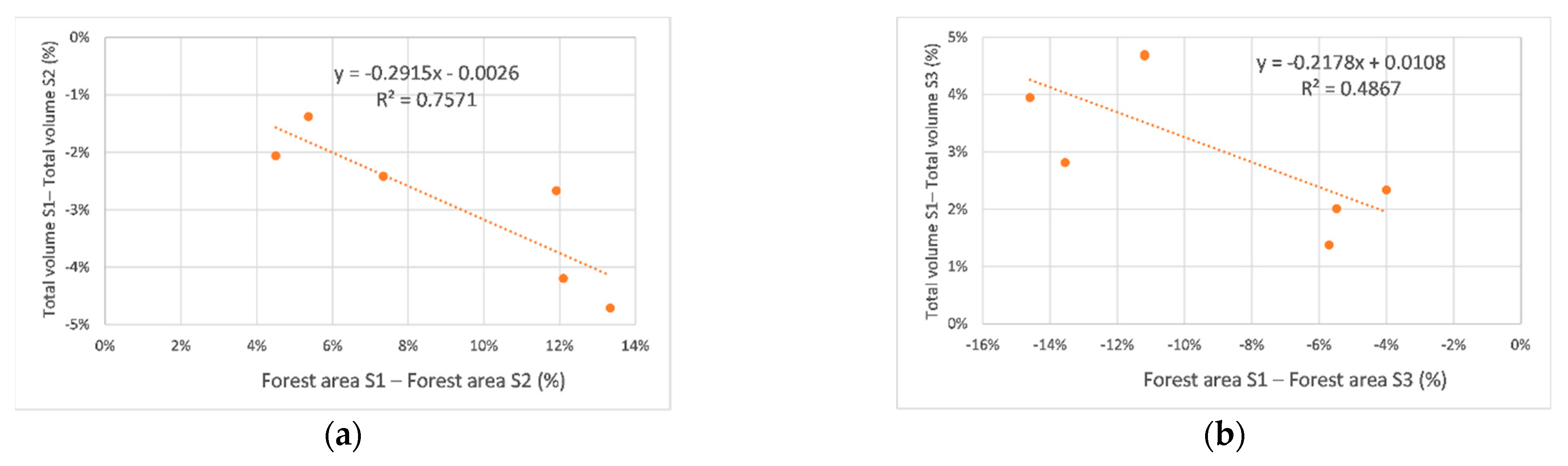
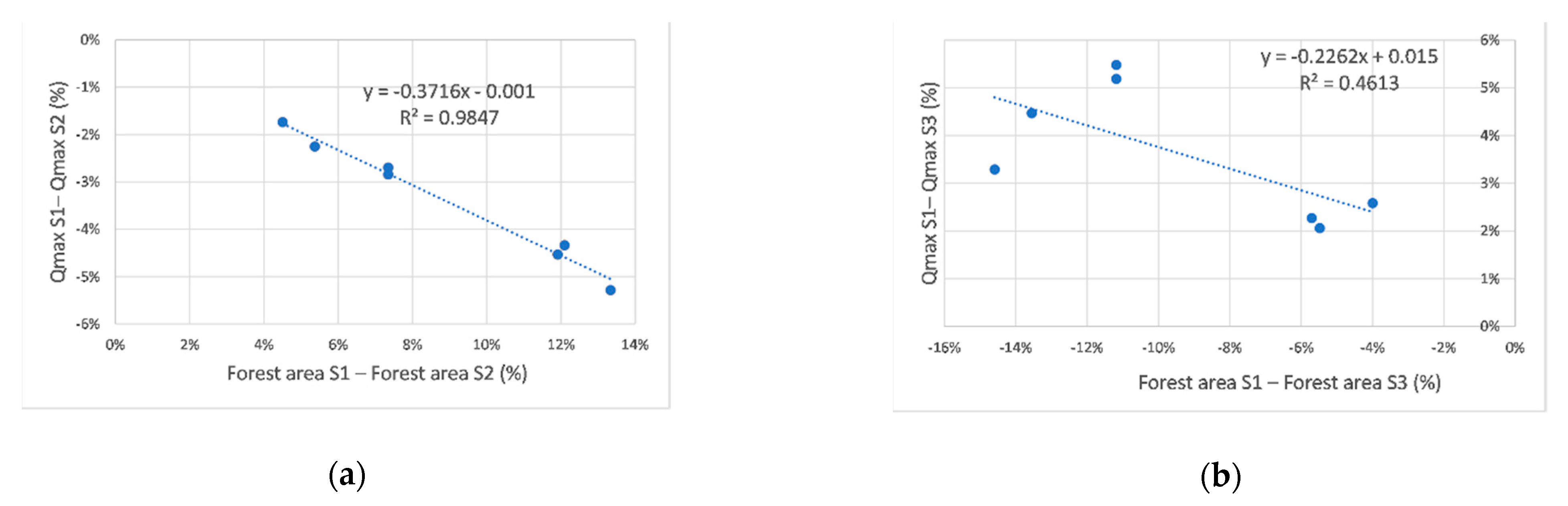
3.2. The Impact of Changes in Forested Areas on Peak Flood Discharges

As described in the methodology chapter, we used three scenarios to assess the impact of forest vegetation on runoff.

By modifying the values of the forested areas, according to S2 and S3, the values of the average CN will also change. The change in average CN values leads to changes in the estimated volume and flow values.

The results of the simulations for the three scenarios are presented in Figure 13 and

Table 5. The result of the simulations on the 3 scenarios.

Scenario	Event Period	Total Volume (106 m3) Simulated	Total Volume (106 m3) Observed	Difference V Observed–Simulated (%)	Q Max (m3/s) Simulated	Q Max (m3/s) Observed	Difference Q Observed (S1)–Simulated (%)	Difference Q Compared to S1
S1	4 September 1992–10 September 1992	4.873	5.623	13.35%	14.245	18.6
S2		4.758	5.623	15.39%	13.851	18.6	25.53%	−2.84%
S3		5.112	5.623	9.10%	15.070	18.6	18.97%	8.09%
S1	4 July 1998–10 July 1998	12.16	11.544	−5.35%	40.710	31.7
S2		11.672	11.544	−1.11%	39.018	31.7	−23.09%	−4.34%
S3		12.411	11.544	−7.51%	41.567	31.7	−31.13%	6.13%
S1	17 June 2001–23 June 2001	4.182	4.637	9.81%	14.334	14.8
S2		4.083	4.637	11.94%	13.958	14.8	5.69%	−2.70%
S3		4.388	4.637	5.36%	15.119	14.8	−2.16%	7.68%
S1	21 July 2008–29 July 2008	13.598	16.271	16.43%	44.685	57.6		-
S2		13.324	16.271	18.11%	43.923	57.6	23.74%	−1.74%
S3		14.157	16.271	12.99%	46.205	57.6	19.78%	3.29%
S1	10 September 2013–15 September 2013	1.227	1.176	−4.30%	5.194	3.78
S2		1.210	1.176	−2.88%	5.079	3.78	−34.39%	−2.25%
S3		1.262	1.176	−7.32%	5.437	3.78	−43.84%	6.57%
S1	24 June 2015–27 June 2015	1.173	1.272	7.76%	7.507	6.24
S2		1.121	1.272	11.91%	7.131	6.24	−14.28%	−5.28%
S3		1.201	1.272	5.55%	7.706	6.24	−23.51%	7.47%
S1	24 July 2017–27 July 2017	0.647	1.256	48.49%	4.490	5.659
S2		0.630	1.256	49.83%	4.295	5.659	24.10%	−4.53%
S3		0.656	1.256	47.77%	4.594	5.659	18.82%	6.51%

. Once the model is set and calibrated, according to the methodology described in Section 2, the runoff hydrograph is analyzed for each year event (Figure 14).

The results of the simulations on the three scenarios show an important influence of forests in reducing the peak flows. This influence is preserved up to a fairly significant share of the drained volume during floods (Table 5 and Figure 14). Even if the differences between the forest surfaces determined for different years and the values S2 and S3 are not very high, analyzing Table 5, we can observe an influence exerted on the peak flow, varying between −5.28% (S2) and 8.09% (S3).

The influence of forests in attenuating flood peaks is visible. The weight of this influence can be determined by drawing the correlation graph based on the surface differences of the three scenarios with the cumulated runoff volumes on each scenario:

Forest area S1–forest area S2 compared with total volume S1–total volume S2 (Figure 14a);

Forest area S1–forest area S3 compared with total volume S1–total volume S3 (Figure 14b).

The result of this analysis is shown in the two graphs of Figure 15.

In the focus region, the catchment response to the increase in the forested surface was the reduction in the total runoff volumes for the selected event (Figure 15a). In the case of a decrease in the forested area (scenario S3), the total runoff increased during the analyzed event (Figure 15b).

A similar situation was detected when comparative analysis was performed for the maximum runoff during the considered events (Figure 16). In this case, the analyses were conducted considering the following differences:

-

Difference between forest area S1 and forest area S2 was compared with the difference between maximum runoff S1 and maximum runoff S2 (Figure 16a);

-

Difference between forest area S1 and forest area S3 was compared with the difference between maximum runoff S1 and maximum runoff S3 (Figure 16b).

A negative value of differences was obtained in all the graphs presented in Figure 15 and Figure 16, where an increase in the forested area corresponds to a decrease in the maximum flow and vice versa. Additionally, the Pearson squared correlation index R² in both Figure 15a and Figure 16a (i.e., the relation between S1 and S2) indicated a stronger correlation compared to the relations S1–S3 (Figure 15b and Figure 16b). Given the similar direction for both types of relations, S1–S2 and S1–S3, regardless of whether they are about the volume or flows, one can choose the best correlation. The correlation index presented in Figure 16a has the highest value, which is why we can use it as an equation in estimating the share of influence of forests on runoff (Equation (15):

y = −0.3716x − 0.001

(15)

where:

y—the estimate percentage of the maximum flow;

x—the percentage of the forested area related to the reference value S1;

0.3717—slope of the regression line;

−0.001—Y axis intercept.

3.3. Limitations

The analysis of the vegetation indices in order to determine the forest surface was conducted on satellite images, which have a low spatial resolution (30 m), and this can influence the results. However, the accuracy analysis of the method was performed on the orthophoto images from 2018, which have a 5 cm/pixel resolution. An analysis conducted on satellite images with a better spatial accuracy would lead to a much more accurate result, but in this paper, we aimed to find the order of magnitude of this influence.

Another limitation of the method is the quality and time step of precipitation data. We used daily gridded datasets with a spatial resolution of 0.1°. For this type of analysis on small catchments, it is recommended to use hourly precipitation because of the short concentration time and to perform a comparative analysis of the data contained within the observed values [27] to determine the quality of the data contained in the gridded dataset. However, hourly data are not available for the area under study.

The model used in these analyses is designed to simulate events in which the snow parameter has no influence. Therefore, in choosing the event for simulation, it is essential that the snow or melting snow does not exert any influence.

4. Discussion

LULCC represents one of the most important factors that alter natural runoff regimes. The uncertainties in many studies were linked to the type of land use change. Among all types of land use, forests seem to play a role of crucial importance in the soil–water–atmosphere system [42]. Previous studies developed worldwide considered that the most important influence must be attributed to forested areas. Thus, a recent study in a mountain region in Brazil stated that “an increase in forest area is expected to decrease surface runoff and the associated water yield, and may mitigate the impacts of extreme precipitation events” [7]. Several other studies concluded that land use plays an essential role in determining the amount of percolating water, surface runoff and the lost water to the atmosphere through evapotranspiration [42,43].

In this research, we tried to capture and quantify the importance of forests. To achieve this objective, the study area was chosen taking into account the idea that the catchment should be small and controlled hydrometrically and have significant areal afforestation and deforestation change over time.

In fact, our correlations underlined that the forested area decrease contributed to the growth in the runoff water volume and discharge. Moreover, our results emphasize the importance of forests in the presented phenomena, where a forested area increase corresponds to a decrease in maximum flow, in agreement with the current literature findings, which reveal that deforestation leads to an immediate increase in the total discharge and the maximum flow [43].

In Romania, the areas covered with forests and their density have evolved over the years. Before 1989 (the year when the communist system collapsed in Eastern Europe), more attention was paid to forests to increase their economic efficiency; after 1989, there was a series of deforestation actions, both natural and anthropogenic (most of them illegal) [35].

After 2003, a new forest law was implemented, which stopped the advance of illegal deforestation, and after 2015, with the implementation of the “forest radar” application, this measure was intensified. Throughout the period, however, the administrator of the forest ROMSILVA tried numerous actions to reforest the deforested slopes. The results of these administrative measures are slowly beginning to show their results through a steady increase in forested areas.

5. Conclusions

Forested areas in river basins play an imperative role in attenuating flood peaks. One of the questions that this article wanted to answer is the quantification of this influence. This objective is covered by the PannEx project Flagship Question 4 [7]. According to the PannEx White Book, it is crucial to assess all anthropogenic influences which could alter the original natural water cycle, which, in part, represents the only true image regarding the available water resources [44].

The use of satellite images can be a valuable source of information regarding the extent of forested areas. Especially in mountainous areas, but not only in these areas, it is vital to consider that the entire land is not suitable for afforestation, either due to the vertical vegetation steps (alpine vegetation, areas of juniper and dwarf trees, moorland, etc.) or due to steep slopes or bare terrain. This type of analysis, based on successive time series assessments, can help to determine the maximum area that is suitable for afforestation.

Another advantage of this method is the use of freely available gridded datasets, meaning they can be used by any authority in order to evaluate the possible impact the extension or reduction in the forest surface would have.

The delineation of the forested area for certain regions (and at a certain date) can often be difficult to achieve for various reasons. Often the plans or maps held by the forest administrator do not provide a complete or real picture of the forested area, or the magnitude of deforestation or afforestation. Extraction of the FCD vegetation index based on Landsat images can be an important and relevant source of information regarding the delineation of the forested area. The results obtained in this research are encouraging and recommend the use of such a method for delimiting forested areas.

The analysis of the model results, performed on three scenarios, allows us to deduce a simple equation for estimating the influence of the forest surface on the maximum river flows. The use of such an equation allows us to hypothetically determine the percentage by which the maximum flow rate increases or decreases depending on the decrease or increase in the forest area.

In Romania, over recent decades, a lot of money has been invested in large-scale water works regarding structural measures for the attenuation of flood waves by dam constructions, accumulations, non-permanent accumulations, etc. This type of analysis revealed that for certain areas of the catchment, reforestation measures are enough to reduce the flood peaks, or to remove the negative effect of floods. Thus, by using this method, a lot of money and effort can be saved and can be invested in the quality of people’s lives.

As further work, to test this method for areas with lower slopes, or hill or plain areas, identifying where the forest can play an even more important role is a priority. Furthermore, using the satellite images provided by the Copernicus Sentinel missions, with a much better resolution, could improve the results.

References

1. Vazken, A. Waters and forests: From historical controversy to scientific debate. J. Hydrol. 2004, 291, 1–27. [Google Scholar] [CrossRef]
2. De Niel, J.; Willems, P. Climate or land cover variations: What is driving observed changes in river peak flows? A data-based attribution study. Hydrol. Earth Syst. Sci. 2019, 23, 871–882. [Google Scholar] [CrossRef]
3. Arheimer, B.; Lindström, G. Detecting changes in river flow caused by wildfires, storms, urbanization, regulation, and climate across Sweden. Water Resour. Res. 2019, 55, 8990–9005. [Google Scholar] [CrossRef]
4. Bernsteinová, J.; Bässler, C.; Zimmermann, L.; Langhammer, J.; Beudert, B. Changes in runoff in two neighbouring catchments in the Bohemian Forest related to climate and land cover changes. J. Hydrol. Hydromech. 2015, 63, 342–352. [Google Scholar] [CrossRef] [Green Version]
5. Kim, G.S.; Lim, C.-H.; Kim, S.J.; Lee, J.; Son, Y.; Lee, W.-K. Effect of National-Scale Afforestation on Forest Water Supply and Soil Loss in South Korea, 1971–2010. Sustainability 2017, 9, 1017. [Google Scholar] [CrossRef] [Green Version]
6. Adams, H.D.; Guardiola-Claramonte, M.; Barron-Gafford, G.A.; Villegas, J.C.; Breshears, D.D.; Zou, C.B.; Troch, P.A.; Huxman, T.E. Temperature sensitivity of drought-induced tree mortality portends increased regional die-off under global-change-type drought. Proc. Natl. Acad. Sci. USA 2009, 106, 7063–7066. [Google Scholar] [CrossRef] [PubMed] [Green Version]
7. Kiprotich, P.; Wei, X.H.; Zhang, Z.K.; Ngigi, T.; Qiu, F.T.; Wang, L.H. Assessing the Impact of Land Use and Climate Change on Surface Runoff Response Using Gridded Observations and SWAT+. Hydrology 2021, 8, 48. [Google Scholar] [CrossRef]
8. Ceglar, A.; Croitoru, A.-E.; Cuxart, J.; Djurdjevic, V.; Güttler, I.; Ivančan-Picek, B.; Jug, D.; Lakatos, M.; Weidinger, T. PannEx: The Pannonian Basin Experiment. Clim. Serv. 2018, 11, 78–85, ISSN 2405-8807. [Google Scholar] [CrossRef]
9. Hallegatte, S.; Green, C.; Nicholls, R.J.; Corfee-Morlot, J. Future flood losses in major coastal cities. Nat. Clim. Chang. 2013, 3, 802–806. [Google Scholar] [CrossRef]
10. Knapp, A.K.; Beier, C.; Briske, D.D.; Classen, A.T.; Luo, Y.; Reichstein, M.; Heisler, J.L. Consequences of more extreme precipitation regimes for terrestrial ecosystems. Bioscience 2008, 58, 811–821. [Google Scholar] [CrossRef]
11. Croitoru, A.-E.; Piticar, A.; Burada, D.C. Changes in precipitation extremes in Romania. Quat. Int. 2016, 415, 325–335, ISSN 1040-6182. [Google Scholar] [CrossRef]
12. Croitoru, A.-E.; Minea, I. The impact of climate changes on rivers discharge in Eastern Romania. Theor. Appl. Climatol. 2015, 120, 563–573. [Google Scholar] [CrossRef]
13. Pollner, J.; Kryspin-Watson, J.; Nieuwejaar, S. Disaster Risk Management and Climate Change Adaptation in Europe and Central Asia; The World Bank and Global Facility for Disaster Reduction and Recovery: Washington, DC, USA, 2010. [Google Scholar]
14. Azizi, Z.; Najafi, A.; Sohrabi, H. Forest Canopy Density Estimating, Using Satellite Images. Int. Arch. Photogramm. Remote. Sens. Spat. Inf. Sci. 2008, XXXVII, 1127–1130. [Google Scholar]
15. Bradshaw, C.J.A.; Sodhi, N.S.; Peh, K.S.-H.; Brook, B.W. Global evidence that deforestation amplifies flood risk and severity in the developing world. Glob. Chang. Biol. 2007, 13, 2379–2395. [Google Scholar] [CrossRef]
16. Bonell, M. Progress in the understanding of runoff generation dynamics in forests. J. Hydrol. 1993, 150, 217–275. [Google Scholar] [CrossRef]
17. Ian, R. Calder and Bruce Aylward, Forests and Floods: Moving to an Evidence-based Approach to Watershed and Integrated Flood Management. Water Int. 2006, 31, 541–543. [Google Scholar] [CrossRef]
18. Kabeja, C.; Li, R.; Guo, J.; Rwatangabo, D.E.R.; Manyifika, M.; Gao, Z.; Wang, Y.; Zhang, Y. The Impact of Reforestation Induced Land Cover Change (1990–2017) on Flood Peak Discharge Using HEC-HMS Hydrological Model and Satellite Observations: A Study in Two Mountain Basins, China. Water 2020, 12, 1347. [Google Scholar] [CrossRef]
19. Park, J.Y.; Ahn, S.R.; Hwang, S.J.; Jang, C.H.; Park, G.A.; Kim, S.J. Evaluation of MODIS NDVI and LST for indicating soil moisture of forest areas based on SWAT modeling. Paddy Water Environ. 2014, 12, 77–88. [Google Scholar] [CrossRef]
20. Dwarakish, B.P. Ganasri. Impact of land use change on hydrological systems: A review of current modeling approaches. Cogent Geosci. 2015, 1, 1115691. [Google Scholar] [CrossRef]
21. Martin, N. Risk Assessment of Future Climate and Land Use/Land Cover Change Impacts on Water Resources. Hydrology 2021, 38, 38. [Google Scholar] [CrossRef]
22. Romanian National Projects~Flood Risk Management Plan of Someș—Tisa Water Basin Administration. 2016. Available online: https://rowater.ro (accessed on 15 February 2021).
23. Romanian National Projects~Plan for the Prevention, Protection and Mitigation of the Effects of Floods on the Someș—Tisa Water Basin PPPDEI (2014), (Planul Pentru Prevenirea, Protecția și Diminuarea Efectelor Inundațiilor în Bazinul Hidrografic Someș Tisa, in Romanian). Available online: http://www.rowater.ro/dasomes/Documente/Proiect%20PPPDEI/PPDEI_varianta_initiala.pdf (accessed on 15 February 2021).
24. Romanian Law no. 107/1996—“Water Law”, with Subsequent Amendments and Completions (Legea nr. 107/1996—Legea Apelor, cu Modificările şi Completările Ulterioare); Autonoma, R. (Ed.) Monitorul Oficial: Bucureşti, Romania; Available online: http://www.vertic.org/media/National%20Legislation/Romania/RO_Water_Law_1996.pdf (accessed on 14 May 2021).
25. Cornes, R.; van der Schrier, G.; van den Besselaar, E.J.M.; Jones, P.D. An Ensemble Version of the E-OBS Temperature and Precipitation Datasets. J. Geophys. Res. Atmos. 2018, 123. [Google Scholar] [CrossRef] [Green Version]
26. Website of the European Climate Assessment & Dataset Project. Available online: https://www.ecad.eu/ (accessed on 15 February 2021).
27. Sidău, M.R.; Croitoru, A.-E.; Alexandru, D.E. Comparative analysis between daily extreme temperature and precipitation values derived from observation and gridded datasets in northwestern Romania. Atmosphere 2021, 12, 361. [Google Scholar] [CrossRef]
28. Website of USGS Global Visualization Viewer (GloVis). Available online: http://glovis.usgs.gov/ (accessed on 15 February 2021).
29. Geoportal ANCPI. Available online: https://geoportal.ancpi.ro/portal/ (accessed on 17 February 2021).
30. Pompiliu, M. The Runoff Coefficient of the Water in Rivers (in Romanian—Coeficientul de Scurgere a Apei în Râuri); Edit Academiei: București, România, 2019. [Google Scholar]
31. Roy, P.; Rikimaru, A.; Miyatake, S. Tropical forest cover density mapping. Trop. Ecol. 2002, 43, 39–47. [Google Scholar]
32. Rikimaru, A. The Concept of FCD Mapping Model and Semi-Expert System. FCD Mapper User’s Guide; International Tropical Timber Organization and Japan Overseas Forestry Consultants Association: Yokohama, Japan, 1999; p. 90. [Google Scholar]
33. Loi, D.T.; Chou, T.-Y.; Fang, Y.-M. Integration of GIS and Remote Sensing for Evaluating Forest Canopy Density Index in Thai Nguyen Province, Vietnam. Int. J. Environ. Sci. Dev. 2017, 8, 539–542. [Google Scholar] [CrossRef] [Green Version]
34. Jennings, S.; Brown, N.; Sheil, D. Assessing Forest Canopies and Understorey Illumination: Canopy Closure, Canopy Cover and Other Measures. Forestry 1999, 71, 59–73. [Google Scholar] [CrossRef]
35. Dragoi, M.; Toza, V. Did Forestland Restitution Facilitate Institutional Amnesia? Some Evidence from Romanian Forest Policy. Land 2019, 8, 99. [Google Scholar] [CrossRef] [Green Version]
36. Mihai, B. Remote Sensing. Introduction to Digital Image Processing (in Romanian—Teledetectie. Vol 1. Procesarea Digitala a Imaginilor); Universitatii din Bucuresti: Bucuresti, Romania, 2007; p. 208. [Google Scholar]
37. Mchugh, M.L. Interrater reliability: The kappa statistic. Biochem. Med. 2012, 276–282. [Google Scholar] [CrossRef]
38. DHI. MIKE 11: A Modeling System for Rivers and Channels; Reference Manual; Danish Hydraulic Institute: Hørsholm, Denmark, 2017. [Google Scholar]
39. Soil Conservation Service. National Engineering Handbook, Section 4, Hydrology; Department of Agriculture: Washington, DC, USA, 1972; 762p.
40. Kocsis, I.; Haidu, I.; Maier, N. Application of a Hydrological Mike Hydro River—UHM Model for Valea Rea River (Romania). Case Study, Flash Flood Event Occurred On 1 August 2019. In Proceedings of the Air and Water–Components of the Environment, Cluj-Napoca, Romania, 20–22 March 2020. [Google Scholar] [CrossRef]
41. Chendeş, V. Water Resources in Curvature Subcarpathians. Geospatial Assessments (in Romanian—Resursele de Apă Din Subcarpaţii de la Curbură. Evaluări Geospaţiale; Romanian Academy Publishing: Bucharest, Romania, 2011. [Google Scholar]
42. Gomes, L.C.; Bianchi, F.J.J.A.; Cardoso, I.M.; Schulte, R.P.O.; Fernandes, R.B.A.; Fernandes-Filho, E.I. Disentangling the historic and future impacts of land use changes and climate variability on the hydrology of a mountain region in Brazil. J. Hydrol. 2021, 594, 125650. [Google Scholar] [CrossRef]
43. Truong, N.C.Q.; Nguyen, H.Q.; Kondoh, A. Land Use and Land Cover Changes and Their Effect on the Flow Regime in the Upstream Dong Nai River Basin, Vietnam. Water 2018, 10, 1206. [Google Scholar] [CrossRef] [Green Version]
44. Bartholy, J.; Bartók, B.; Bede-Fazekas, Á.; Belušić, A.; Bihari, Z.; Birkás, M.; Bozó, L.; Brmež, M.; Brozović, B.; Ceglar, A.; et al. PannEx White Book, A GEWEX Regional Hydroclimate Project (RHP) over the Pannonian Basin; WCRP Report 3/2019; World Climate Research Programme (WCRP): Geneva, Switzerland, 2019; p. 108. [Google Scholar]
Figure 1. Study area and location of the considered hydrometrical station.
Atmosphere 12 00817 g001
Figure 2. Land use of the Ruscova River according to Corine Land Cover 2018.
Atmosphere 12 00817 g002
Figure 3. Flow chart of FCD mapping model.
Atmosphere 12 00817 g003
Figure 4. Advanced vegetation index (AVI). (a) AVI 1989, (b) AVI 2017.
Atmosphere 12 00817 g004
Figure 5. Bar soil index (BI). (a) BI for year 1989; (b) BI for year 2017.
Atmosphere 12 00817 g005
Figure 6. Shadow index (SI). (a) SI for year 1989; (b) SI for year 2017.
Atmosphere 12 00817 g006
Figure 7. Thermal index (TI). (a) TI for year 1989; (b) TI for year 2017.
Atmosphere 12 00817 g007
Figure 8. Forest canopy density (FCD). (a) FCD for year 1989; (b) FCD for year 2017.
Atmosphere 12 00817 g008
Figure 9. Thematic map layers used in model. (a) Altitude; (b) Slope angle; (c) Soil texture; (d) Daily gridded precipitation databases.
Atmosphere 12 00817 g009
Figure 10. Isolation of an event on the hydrograph: (a) 1992 and (b) 2001.
Atmosphere 12 00817 g010
Figure 11. The evolution of the forested area.
Atmosphere 12 00817 g011
Figure 12. FCD index extracted from satellite images. (a) FCD 1985; (b) FCD 1989; (c) FCD 1992; (d) FCD 2001; (e) FCD2003; (f) FCD 2008; (g) FCD 2013; (h) FCD 2015; (i) FCD 2017.
Atmosphere 12 00817 g012
Figure 13. The values of the CN taken into account in the calibration.
Atmosphere 12 00817 g013
Figure 14. Simulated and observed instantaneous unit hydrograph results. (a) Runoff and Q acumulated—1992; (b) Runoff and Q acumulated—2001; (c) Runoff and Q acumulated—2008; (d) Runoff and Q acumulated—2013.
Atmosphere 12 00817 g014
Figure 15. Comparative analysis of the total volume of water drained during the events and the differences in forested areas, between the three scenarios S1, S2 and S3. (a) S1 compared with S2; (b) S1 compared with S3.
Atmosphere 12 00817 g015
Figure 16. Comparative analysis for the maximum value of water flow during events and differences in forested areas, between the three scenarios S1, S2 and S3. (a) S1 compared with S2; (b) S1 compared with S3.
Atmosphere 12 00817 g016