Abstract
In this paper, we study, in theoretical terms, the structure of the spectrum of acoustic-gravity waves (AGWs) in the nonisothermal atmosphere having asymptotically constant temperature at high altitudes. A mathematical problem of wave propagation from arbitrary initial perturbations in the half-infinite nonisothermal atmosphere is formulated and analyzed for a system of linearized hydrodynamic equations for small-amplitude waves. Besides initial and lower boundary conditions at the ground, wave energy conservation requirements are applied. In this paper, we show that this mathematical problem belongs to the class of wave problems having self-adjoint evolution operators, which ensures the correctness and existence of solutions for a wide range of atmospheric temperature stratifications. A general solution of the problem can be built in the form of basic eigenfunction expansions of the evolution operator. The paper shows that wave frequencies considered as eigenvalues of the self-adjoint evolution operator are real and form two global branches corresponding to high- and low-frequency AGW modes. These two branches are separated since the Brunt–Vaisala frequency is smaller than the acoustic cutoff frequency at the upper boundary of the model. Wave modes belonging to the low-frequency global spectral branch have properties of internal gravity waves (IGWs) at all altitudes. Wave modes of the high-frequency spectral branch at different altitudes may have properties of IGWs or acoustic waves depending on local stratification. The results of simulations using a high-resolution nonlinear numerical model confirm possible changes of AGW properties at different altitudes in the nonisothermal atmosphere.
1. Introduction
Studies of spacetime variations in the upper atmosphere and ionosphere have reliably revealed connections between disturbances in the upper atmosphere and ionosphere and the processes occurring in the troposphere near the Earth’s surface [1,2,3,4]. One of the mechanisms ensuring such connections could be the upward propagation of acoustic waves (AWs) and internal gravity waves (IGWs). These waves generated by various sources can propagate into the middle and upper atmosphere, break, and produce different kinds of perturbations [5,6]. Dissipating waves may generate jet streams and change the heat balance in the upper atmosphere [7,8,9]. Atmospheric waves reaching the ionosphere can affect plasma motions and, consequently, the radio wave propagation [10,11]. Active developments of the theory of waves in the atmosphere began in the twentieth century [11,12,13,14]. Physical mechanisms of the propagation of infrasound and IGWs in the atmosphere are determined by the pressure gradient and gravity forces acting on the atmospheric gas under the conditions of a stratified medium. Currently, many experimental and theoretical results have showed substantial impact of waves on the atmospheric dynamics [7,15,16].
Often, AWs and IGWs are combined into a class of atmospheric acoustic-gravity waves (AGWs) [11,16,17,18,19]. Some current terminology problems in the theory and experimental studies of atmospheric waves are discussed in [14]. The terms AW and IGW appeared in the scientific literature in the context of theoretical analysis of hydrodynamic equations for waves in the isothermal atmosphere, when the background temperature does not depend on altitude [11,12,13,14]. Two different wave branches with significantly different properties were found in the solutions of these wave equations [20]. One branch contains AWs with frequencies always greater than the acoustic cutoff frequency [14]. The second wave branch contains IGWs (or buoyancy waves) with frequencies always lower than the Brunt–Vaisala frequency N [20,21]. In the isothermal model, always and, in the lower atmosphere, AWs as well have periods less than 4.9 min, while IGW periods are greater than min.
However, isothermal approximation for waves could only be valid in a relatively small vicinity of the altitude under consideration [11,13,20,22]. Various attempts were made to take realistic atmospheric temperature profiles into account and to modify the dispersion equation for better identification of AW and IGW branches in the nonisothermal atmosphere. The most common WKB method considers waves that are sufficiently short at an altitude in order to introduce local corrections to and N, taking the temperature gradients into account [14]. Estimates show that such corrections may reach up to 10% [23], and layers may appear in the nonisothermal atmosphere, where and the frequencies of the acoustic and gravity wave branches may overlap. If one considers wave propagation at altitudes from the ground up to thermosphere, then the background temperature gradients change by several times, and the atmosphere with realistic stratification should be considered as fundamentally nonisothermal. Therefore, a rigorous analysis of the behavior of different branches of eigenfunctions of the wave equations in the realistic nonisothermal atmosphere is required for better understanding of wave properties.
A classification of wave types in the spherical rotating atmosphere was studied, for example, by Dikij [12]. He suggested that the atmospheric scale height is infinitely rising at heights . However, observations and atmospheric models show that the background atmospheric state tends to be quasi-isothermal in the nondisturbed upper thermosphere due to high diffusion and thermal conductivity (see Figure 1 below). Therefore, the analysis of atmospheric wave eigenvalues and eigenfunctions must take these upper boundary conditions into consideration.
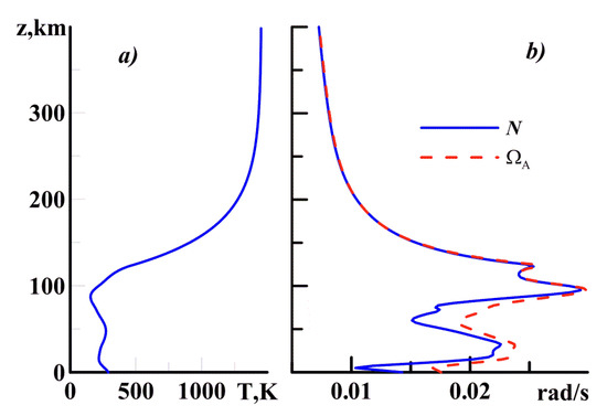
Figure 1.
An example of vertical profile of the background temperature [28] in July at latitude N (a) and respective profiles of the Brunt–Vaisala N and acoustic cutoff frequencies (b) given by Equation (25).
In this paper, we mathematically study the linearized hydrodynamic equations for small-amplitude waves in the realistic nonisothermal atmosphere at altitudes from the ground to infinity. We consider a wide class of realistic stratifications, for which the atmosphere’s scale height reaches an absolute finite maximum value of at . In mathematical terms, the issue of wave branches is equivalent to studying the structure of a continuous spectrum of the wave operator that depends on the eigenvalues (frequencies) of eigenfunctions (wave modes) in the nonisothermal model.
It is shown below that, in the realistic nonisothermal atmosphere, the wave operator is self-adjoint and its spectrum contains two “global” wave branches of acoustic-gravity waves with frequencies lower and higher than and , respectively (see Equation (20) below), which are the Brunt–Vaisala and acoustic cutoff frequencies for the upper quasi-isothermal layer of the atmosphere. Similar to the theory of waves in the isothermal atmosphere, in which there is a gap between the threshold frequencies > , there is a gap between the high- and low-frequency global branches. However, the values of and depend on the atmospheric parameters near the upper boundary (at infinity) and may differ from local values of and in the lower and middle atmosphere. Therefore, wave modes corresponding to both global wave branches of acoustic-gravity waves may have properties of IGWs at some altitudes and properties of AWs at other altitudes depending on local values of and in the nonisothermal atmosphere, as discussed in Section 5.
2. Mathematical Problem of Atmospheric Wave Propagation
In this section, the problem of propagation of waves generated by initial disturbances in the nonisothermal atmosphere is formulated mathematically.
2.1. Hydrodynamic Equations and Boundary Conditions
Let us consider a system of nondissipative linear equations for small-amplitude acoustic-gravity waves in the plane nonrotating atmosphere [11,13,14,20,24]:
where g is gravitational acceleration; is the ratio of heat capacities at constant pressure and volume; is the atmosphere’s scale height; stratification parameter at all altitudes z; is atmospheric density; zero indices refer to the stationary background values; u and w are the horizontal and vertical velocity components; and functions
are relative perturbations of pressure, density, and temperature. The equation system (1) does not take the viscosity and thermal conductivity, which are insignificant for relatively long waves, into account. The system (1) for the nonrotating plane atmosphere is applicable for AGWs with periods and horizontal wavelengths substantially smaller than a day and the Earth’s radius, respectively. With the x-axis directed along the horizontal wave vector, the 2D model (1) can adequately describe the propagation of small-amplitude acoustic-gravity waves in the stratified atmosphere. The lower boundary condition at the ground has the following form in our model:
In this paper, we consider the atmosphere extending to infinity in altitude, and the upper boundary conditions depend on the stratification. Many experiments and theoretical studies [2,3,4,25,26,27] show that AGWs in the upper atmosphere frequently propagate upwards from wave sources located at lower altitudes. Therefore, the upper boundary conditions should avoid wave reflections at high atmospheric altitudes. From the equation system (1), using standard transformations [12,14], one can get the following equation for the wave energy:
where e and are the densitiy of the wave energy and its flux, respectively. The three terms in the expression for e in (4) are sometimes called densities of kinetic, elastic, and thermobaric energy [12], which are respectively connected with wave motions, compressions, and buoyancy forces acting on atmospheric parcels vertically shifted from the equilibrium state. Equation (4) determines local changes of wave energy [25].
One can integrate One can integrate (4) over entire regions and . Wave energy fluxes crossing the upper and lower boundaries are equal to zero, because waves cannot reach infinite distance at any finite time and due to the condition (3) at the Earth’s surface. Therefore, the divergence theorem leads to the conservation law of the total (integral) wave energy E:
The conservation of total wave energy (5) is used for the selection of physically justified solutions in this model.
2.2. Initial Conditions
The traditional mathematical problem of wave propagation from an initial perturbation in the semi-infinite atmosphere assumes the following initial conditions for the equation system (1):
Here, functions , , , are components of the initial velocity vector, initial relative density, and relative temperature, respectively. The lower boundary condition at the ground has the form of (3). An addition condition corresponding to the conservation of total wave energy (5) is applied:
We use this requirement instead the horizontal and upper boundary conditions. The existence of integral (4) assumes that functions u, w, , and should decrease at and may grow at , but no faster than . The local form of the wave energy Equation (4) is obtained from the main equation system(1), taking physical reasons for zero wave energy fluxes at the upper boundary (infinity) into account. Therefore, Equation (7) is not the direct consequence of Equation (1), but rather, an additional requirement reflecting the upper boundary conditions.
2.3. Atmospheric Stratification
Figure 1 shows an example of typical vertical profile of the background temperature for July at middle northern latitudes at high solar activity, corresponding to the solar radio flux F107 = 250, which is calculated using the NRLMSISE-00 model [28]. Figure 1 of the [25] shows the behavior of temperature profiles at high altitudes for low and moderate solar activity similar to Figure 1a. The dependence is similar to Figure 1a since g and atmospheric molecule mass vary at different altitudes more slowly than the background temperature. Therefore, in this study, we assume that in the undisturbed high atmosphere, the height scale is monotonically increasing at high altitudes and it reaches an absolute finite maximum at . Therefore, we use the following boundary condition:
These assumptions are consistent with temperature behavior in Figure 1a. Equation (8) is different from the assumptions of [12], where at . The differences could be noticeable at high altitudes only; however, they can substantially influence mathematical properties of eigenvalues and eigenfunctions of the analyzed wave operator considered in the following section.
3. Operator Wave Equations
In this section, we consider the atmospheric wave problem in terms of self-adjoint matrix operators in Hilbert spaces. Such operators are frequently used, for example, in quantum mechanics and many mathematical results are known for them. Such operator approaches were almost never applied before for the analysis of atmospheric waves.
3.1. Matrix Wave Equations
The system of the first four wave equations in (1) may be written in the form of a single matrix operator equation having the following form:
where the vector function contains all independent functions of Equation (1) and is a matrix differential operator containing the terms of the left part of (1) depending on spatial derivatives and taking the lower boundary condition (3) into account. For the completeness of the mathematical problem of atmospheric wave propagation, the initial conditions (6) and the requirement of the total wave energy conservation (7) must be added.
The matrix operator does not depend on time t. Therefore, it can be assumed that the solution to (9), , should depend on t parametrically, and one can exclude time from the considerations of the properties of the operator . One can introduce a set of vector functions and use the polarization theorem [29] to determine the scalar product of a pair of functions and as follows:
which is similar to the expression for the local wave energy (4); * denotes complex conjugation. In the Hilbert space of vector functions , in which scalar products of any vector functions and are determined by Equation (10), the expression for total wave energy has the following form:
After these general definitions, the wave problem can be formulated as the search parameterized by t element of the Hilbert space , which satisfies the matrix Equation (9) and the initial conditions (6). The requirement (7) is unnecessary, because for the elements of the Hilbert space the condition of finite total wave energy (11) is satisfied automatically.
3.2. Self-Adjointness of the Wave Operator
An important property can be expressed in the theorem that operator acting from Hilbert space into and having the definition range of
is a self-adjoint operator. The proof of the theorem is standard but bulky. Therefore, we make only some comments here. First, one can verify the expression
using standard integration by parts for a class of continuously differentiated functions with a compact support. Then, one can treat the operator in terms of the Schwartz distribution [29] using (12) for determining , where is a function with compact basis and . Due to the definition range (12), w and should be quadratically integrable within the entire semi-infinite space. Therefore, the lower boundary condition (3) is equivalent to the relation .
The self-adjoint operators have some important properties described in the mathematical literature. First, in 1955, Ladyzhenskaya [30,31] studied operator equations similar to (8) and proved the existence of solutions to this problem. Dikij [12] considered propagation of atmospheric waves in a model of spherical rotating Earth’s atmosphere and proved twofold completeness of eigenfunctions in his model, which means the existence of solutions to the wave problem. However, the author [12] used the “rigid cover” type of the upper boundary condition at an altitude of 200 km, which can cause downward reflections of waves propagating from below. In this respect, setting the upper boundary conditions at infinity helps avoiding reflections of waves propagating from the lower atmosphere in our model. In addition, such conditions allows for these comparison of our results with the traditional theory of acoustic-gravity waves in the semi-infinite atmosphere [14].
The second property of self-adjoint wave operators is the real values of their eigenvalues [29], which satisfy the equation
This equation can be obtained from (9) assuming ; therefore, eigenvalues have the meaning of frequencies of native wave modes (NWMs), which can exist in the entire atmosphere, and their real values show that the amplitudes of these NWMs should be unchanged in time.
The third property of the self-adjoint operators is that eigenfunctions satisfying the Equation (14) form a basis for a function space [29]. This means that any solution of the wave problem (9) with initial conditions (6) can be represented as series expansions in terms of the eigenfunctions corresponding to different NWMs.
4. Eigenfunction Structure
To obtain the general solutions to the wave problem (9), one should study eigenvalues (frequencies) and eigenfunctions (NWMs) corresponding to (14). In the considered stationary plane model, the background atmosphere is homogeneous along the horizontal x-axis. The spatial structure of eigenfunctions for such model (9) may have the following form [12]:
where k is real horizontal wavenumber and is a function describing the vertical structure. Substitution of (15) to (9) leads to the equation for with the operator depending on z only. The scalar product of any pair of functions and has the form similar to (10) with integration over z only. After the substitution of(15), one can transform (9) into a set of two ordinary differential equations for and and algebraic formulae relating these quantities with other wave hydrodynamic fields of Equation (1). At slowly varying background atmospheric characteristics, one One can search for the vertical structure of the wave field in the form of
where is an arbitrary function and the equations for the amplitudes of functions and have the following form:
At high altitudes, in the quasi-isothermal layer (8), one can neglect the left-hand terms of (17) and consider the coefficients in the right-hand side of (17) to be constant. The function in (16) can be set arbitrarily, and in line with the traditional AGW theory [12,14], it can be taken in the following form:
where m is the parameter of this relation, which has the meaning of a vertical wavenumber at high altitudes. In this case, (17) turns into an algebraic equation system
This system has nonzero solutions when its determinant is equal to zero, which gives the following relation valid at :
This formula is similar to the dispersion equation of the traditional AGW theory for the isothermal plane model [14]. However, in the nonisothermal atmosphere, Equation (20) could be valid only at high altitudes, where atmospheric parameters are slowly varying in z. At other altitudes, the equation system (17) can be written in the form of integral equations
where the upper boundary values and are related by the Equation (19), and for , one can use the relation (18). For the realistic nonisothermal atmosphere, the expressions under the integrals in (21) are not equal to zero, but all coefficients are limited and these expressions tend to zero at . Therefore, solutions to the integral Equation (21) exist and are limited. Taking a linear combination of two solutions having form of (16) and (18) and corresponding to and , one can satisfy the lower boundary condition (3). The analysis of Equation (20) similar to [14] reveals for the quasi-isothermal upper layer (8) the existence of two branches of continuous spectrum with real eigenvalues :
where and are respectively the acoustic cutoff and the Brunt–Vaisala frequencies at . Since , these two spectral branches are separated. Equation (22) is similar to the definition of two AGW branches in the traditional isothermal model [14]. In addition, (22) shows that in the nonisothermal atmosphere with conditions (8) at high altitudes, the boundaries of these two “global” AGW frequency branches are determined by the value of and at . However, as discussed in the next section, local properties of wave modes depend on local atmospheric characteristics for all frequencies belonging to both global branches (22).
Linear combinations of wave modes (15) belonging to the continuous spectrum of the wave operator (9) can describe vertical wave propagation.
It is known that the spectrum of a self-adjoint operator, in addition to the continuous part, can contain discrete sets of eigenvalues. Respective wave modes can correspond to the trapped and surface atmospheric waves. The trapped waves can be formed by barriers, which impede the vertical wave propagation, primarily, due to changes in , leading to the formation of waveguides. Near-surface waves, if any are, can propagate along and near the boundary surface.We do not have rigorous proof, but many studies of realistic stratifications and equations for wave modes by WKB approximation show that trapped and near-surface waves are absent for realistic stratifications satisfying Equation (8). As known, in the isothermal atmosphere model, there is a near-surface wave—the Lamb wave [12]. Surface waves require the existence of interfaces between different air masses, along which the waves can propagate.
5. Discussion
The above model does not account for dissipation, background wind, and atmospheric rotation. However, analyses by [26] of the dispersion equation for AGWs dissipating due to molecular and turbulent viscosity and heat conduction with total kinematic coefficient showed that, at a first approximation, the dissipation may influence wave amplitudes, keeping frequencies and wavenumbers unchanged. The background horizontal wind can be taken into account by replacing the observable frequency in the above formulae with the intrinsic frequency [14]:
where is the projection of the background wind on the horizontal wave vector. Earth rotation bound the AGW frequency spectrum to the limit [14]
where f is the Coriolis parameter, is the angular frequency of the Earth rotation, and is latitude. An analytical solution (21) is not possible for arbitrary background profiles and wave parameters.
However, when vertical scales of changes in the background parameters are substantially larger than vertical wavelengths, one can apply the simplified WKB method [14]. The application of this method to Equation (9) shows that the local values of the vertical wavenumbers m are real when
where and are local Brunt–Vaisala and acoustic cutoff frequencies, respectively; is the stratification parameter in (1). These expressions are in line with previous estimations by [12,14] and show influence of the stratification of the nonisothermal atmosphere on the threshold frequencies. Two main kinds of mesoscalel waves are usually considered in the atmosphere, which are produced by different mechanisms. They are AWs produced by compression pressure forces and IGWs produced by buoyancy forces acting on the vertically moving air parcels. These kinds of forces are purified for short waves at high frequencies for AWs and [14]. The main differences between these kinds of waves are in the directions of phase and group speed. For AWs, both speeds are the same and directed perpendicular to wave fronts. IGWs have perpendicular directions of phase and group speeds. The latter is directed along the wave fronts inclined to the horizon and vertical phase velocity has directions opposite to those for group velocity [32]. At other frequencies and wavenumbers, both pressure and buoyancy forces producing acoustic-gravity waves are important. It is significant that the local AGW properties depend on local parameters of waves and stratification.
According to (1) and (25) values of , and become smaller in the atmospheric layers with and larger at . Therefore, one can find minimum and maximum of respective quantities:
Wave modes corresponding to both branches (22) of the global spectrum of eigenvalues of the wave operator (9) can have different properties at different altitudes. Waves with have properties of IGWs at all altitudes. In the atmosphere without substantial instabilities, usually , therefore, this is valid for the entire low-frequency global branch (22) of the wave operator. The high-frequency branch of (22) can be subdivided into two subranges. At frequencies , wave modes everywhere have properties of AWs. In the subrange , wave modes may have properties of IGWs in some layers and properties of AWs in other layers depending on local values of and .
Figure 1a and Figure 1 of the paper [25] corresponds to temperatures of 1500 K, 900 K, and 700 K at altitudes 500–600 km for high, moderate, and low solar activity at F10.7 = 250, 120, 70 sfu, respectively. According to (22), this corresponds to values of s and s. One can see that the global IGW spectral branch becomes more narrow at high solar activity than that at low solar activity.
During active sun events, temperature in the upper thermosphere may dramatically increase and even may have tendencies to quasi-linear increases in height (e.g., [33]). One can anticipate that in this case the IGW global spectral branch may disappear at all and practically wave modes having IGW properties at lower atmospheric layers would have AW properties at high altitudes.
Since usually , some wave modes with of high-frequency branch (22) may have IGW characteristics in the lower and middle atmosphere, but may turn into AW characteristics when frequency becomes when frequency becomes in the quasi-isothermal layer (8) at high altitudes. As far as usually , some IGW modes with propagating in the lower and middle atmosphere may turn into AW modes, when become in the quasi-isothermal layer (8) at high altitudes. Such behavior was frequently found during simulations of atmospheric AGWs with nonlinear 3D high-resolution numerical model “AtmoSym” [34]. Figure 2 shows examples of plane waves (15) with different periods and horizontal wavelengths , which were simulated with the AtmoSym high-resolution model for the background temperature profile shown in Figure 1a. It was shown that the wave fields corresponding to the eigenfunctions of the wave operator (15) can be obtained by specifying plane wave perturbations of vertical velocity at the ground at model times after triggering the surface wave source [35]. Upper boundary conditions in the model were specified at altitude km; at the boundaries of the horizontal atmospheric regions having dimensions of , the periodical conditions described by [27] were specified. The model grid is not equidistant and contains 1536 nodes in altitude and 512 horizontal nodes. All other details of simulations are identical to those described in [25,27].
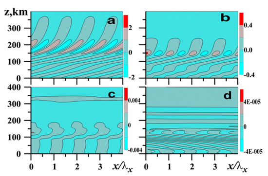
Figure 2.
Simulated vertical velocity w for plane waves with period = 15 min, horizontal wavelength = 90 km at time t = 40 (a); = 7.5 min, = 45 km, t = 40 (b); = 5 min, = 30 km, t = 50 (c); = 0.5 min, = 6 km, t = 90 (d) for the background temperature profile shown in Figure 1.
Figure 2a corresponds to the wave mode with min, which belongs to the low-frequency branch of the global AGW spectrum (22), because . The wave fronts in Figure 2a are inclined to the horizon, the wave energy propagates upwards along the wave fronts, and vertical phase speed is directed downward. This corresponds to the properties of IGWs at all altitudes. Figure 2d corresponds to infrasound wave with period min. In this case, the wave fronts in Figure 2d are also inclined, but in the directions opposite to Figure 2a. The group and phase speeds have the same upward direction perpendicular to the wave fronts. This behavior is characteristic to high-frequency AWs with in (26). In the upper atmosphere, the speed of sound becomes high due to high temperature in Figure 1a, and the wave fronts in Figure 2d become quasihorizontal with vertical wavelengths growing in altitude.
Figure 2b,c represent intermediate wave periods. In Figure 2b for = 7.5 min, one can see IGW structures similar to Figure 2a, but only up to altitudes 200–250 km, where and the wave mode should belong to the local AW type. The vertical wavelength of the corresponding AW in the upper atmosphere exceeds 270 km and respective wave structures are not seen in Figure 2b above the 250 km altitude. Figure 2c is for smaller = 5 min, and one can see complicated wave fronts directions at altitudes below 200 km, which are inclined to the right (similar to Figure 2a) in the regions where and are inclined to the left (similar to Figure 2d) at layers with . At altitudes above 200 km, the vertical wavelength of AWs is larger than 180 km and the distances between quasihorizontal wave fronts in Figure 2c are high. The linear IGW theory predicts total reflection of the wave energy at altitudes, where . However, simulations with the high-resolution model show that wave energy can tunnel through the boundaries between the interfaces between IGWs and AWs and can reach high altitudes.
Examples in Figure 2 show that the analysis of the global spectrum of eigenvalues and eigenfunctions of the wave operator (9) in the atmosphere having a quasi-isothermal layer at high altitudes may help in interpreting numerical experiments and observations of AGWs at all altitudes. Possible changes of the AGW properties at different altitudes should be taken into account in parameterizations of AGW dynamical and thermal impacts in the numerical models of atmospheric circulation, dynamics and thermal regime. Further simulations and observations are required for better understanding of AGW spectrum and properties of wave modes in the realistic nonisothermal atmosphere.
6. Conclusions
A system of linearized hydrodynamic equations (1) describing small-amplitude wave propagation in a nonisothermal plane atmosphere is mathematically analyzed for realistic temperature stratifications (Figure 1). A mathematical problem of AGW propagation from arbitrary initial perturbations (6) having limited energy (7) in the nonisothermal atmosphere having a quasi-isothermal layer near the upper boundary of the model (8) is considered. It is shown that this problem belongs to the group of mathematically well-studied wave problems having self-adjoint evolution operators (9), which proves the correctness (existence) of mathematical solutions for a wide range of possible atmospheric temperature stratifications. Solutions of the problem can be considered as parameterized by time eigenfunctions in an introduced Hilbert space.
A structure of continuous spectrum of eigenvalues of the wave problem of AGW propagation from arbitrary initial perturbations (6) is analyzed. It is shown that wave frequencies considered as eigenvalues of self-adjoint operator (14) are real and form two global branches corresponding to high- and low-frequency AGW modes. These two branches are separated, because in the upper quasi-isothermal layer, the Brunt–Vaisala frequency is smaller than the acoustic cutoff frequency . Usually, is smaller than any local value of given by (25) at lower atmospheric altitudes. Therefore, all wave modes belonging to the low-frequency global branch (22) have properties of IGWs in the entire altitude region. The high-frequency global spectrum branch (22) can be subdivided into two subranges depending on the local values of in (26). At frequencies , the wave modes should have properties of AWs at all altitudes. In the subrange , wave modes may have properties of IGWs at some altitudes and properties of AWs at other altitudes depending on the local values of and . Results of simulations with the high-resolution nonlinear 3D numerical model “AtmoSym” in Figure 2 confirm possible changes of AGW properties at different altitudes in the nonisothermal atmosphere.
Possible changes of AGW properties at different altitudes should be taken into account in parameterizations of AGW dynamical and thermal impacts in the numerical models of atmospheric circulation, dynamics, and thermal regime. Further simulations and observations are required for better understanding of AGW spectrum and properties of wave modes in the realistic nonisothermal atmosphere.
Author Contributions
Conceptualization, S.P.K.; analytical solutions, S.P.K.; writing—original draft preparation, S.P.K. and Y.A.K.; writing—review and editing, N.M.G. All authors have read and agreed to the published version of the manuscript.
Funding
This study was supported by the Ministry of Science and Higher Education of the Russian Federation (agreement 075-15-2021-583) and by the Russian Foundation for Basic Research (grant 19-35-90130).
Conflicts of Interest
The authors declare no conflict of interest.
Abbreviations
The following abbreviations are used in this manuscript:
| AWs | Acoustic waves |
| IGWs | Internal gravity waves |
| AGWs | Acoustic-gravity waves |
| WKB | Wentzel–Kramers–Brillouin approximation |
| NWMs | Native wave modes |
References
- Blanc, E.; Farges, T.; Le Pichon, A.; Heinrich, P. Ten year observations of gravity waves from thunderstorms in western Africa. J. Geophys. Res. Atmos. 2014, 119, 6409–6418. [Google Scholar] [CrossRef]
- Pierce, A.D.; Coroniti, S.C. A mechanism for the generation of acoustic-gravity waves during thunder-storm formation. Nature 1966, 210, 1209–1210. [Google Scholar] [CrossRef]
- Fritts, D.C.; Alexander, M.J. Gravity wave dynamics and effects in the middle atmosphere. Rev. Geophys. 2003, 41, 1003. [Google Scholar] [CrossRef] [Green Version]
- Ratcliffe, J.A. Physics of the Upper Atmosphere; Academic Press: New York, NY, USA, 1960; 586p. [Google Scholar]
- Afraimovich, E.L.; Edemsky, I.K.; Voeykov, S.V.; Yasukevich, Y.V. Spatio-temporal structure of the wave packets generated by the solar terminator. Adv. Space Res. 2009, 44, 824–835. [Google Scholar] [CrossRef]
- Snively, J.B.; Pasko, V.B. Breaking of thunderstorm-generated gravity waves as a source of short-period ducted waves at mesopause altitudes. Geophys. Res. Lett. 2003, 30, 2254. [Google Scholar] [CrossRef] [Green Version]
- Fritts, D.C.; Vadas, S.L.; Mean, K.; Werne, J.A. Wan and variable forcing of the middle atmosphere by gravity waves. J. Atmos. Sol. Terr. Phys. 2006, 68, 247–265. [Google Scholar] [CrossRef]
- Kshevetskii, S.P.; Gavrilov, N.M. Vertical propagation, breaking and effects of nonlinear gravity waves in the atmosphere. J. Atmos. Sol. Terr. Phys. 2005, 67, 1014–1030. [Google Scholar] [CrossRef]
- Karpov, I.; Kshevetskii, S. Numerical study of heating the upper atmosphere by acoustic-gravity waves from a local source on the Earth’s surface and influence of this heating on the wave propagation conditions. J. Atmos. Sol. Terr. Phys. 2017, 164. [Google Scholar] [CrossRef]
- Klimenko, M.; Bessarab, F.; Sukhodolov, T.; Klimenko, V.; Koren’kov, Y.; Zakharenkova, I.; Chirik, N.; Vasil’ev, P.; Kulyamin, D.; Shmidt, K.; et al. Ionospheric Effects of the Sudden Stratospheric Warming in 2009: Results of Simulation with the First Version of the EAGLE Model. Russ. J. Phys. Chem. B 2018, 12, 760–770. [Google Scholar] [CrossRef]
- Grigoriev, G.I. Acoustic-gravity waves in the earth’s atmosphere (Review). Radiophys. Quantum Electron. 1999, 42, 1–21. [Google Scholar] [CrossRef]
- Dikiy, L.A. The Theory of Oscillations of the Earth’s Atmosphere; Hydrometeorological Press: Leningrad, Russia, 1969. [Google Scholar]
- Hines, C. Atmospheric gravity waves. In Thermospheric Circulation; Mir Press: Moscow, Russia, 1975. [Google Scholar]
- Gossard, E.E.; Hooke, W.H. Waves in the Atmosphere; Elsevier Scientific Publishing Company: New York, NY, USA, 1975; 456p. [Google Scholar]
- Ploogonven, R.; Snyder, C. Inertial Gravity Waves Spontaneously Generated by Jets and Fronts. Part I: Different Baroclinic Life Cycles. J. Atmos. Sci. 2007, 64, 2502–2520. [Google Scholar] [CrossRef] [Green Version]
- Plougonven, R.; Zhang, F. Internal gravity waves from atmospheric jets and fronts. Rev. Geophys. 2014, 52, 1–37. [Google Scholar] [CrossRef] [Green Version]
- Sindelarova, T.; Chum, J.; Skripnikova, K.; Base, J. Atmospheric infrasound observed during intense convective storms on 9–10 July 2011, J. Atmos. Sol. Terr. Phys. 2015, 122, 66–74. [Google Scholar] [CrossRef]
- Fovell, R.; Durran, D.; Holton, J.R. Numerical simulation of convectively generated stratospheric gravity waves. J. Atmos. Sci. 1992, 49, 1427–1442. [Google Scholar] [CrossRef] [Green Version]
- Livneh, D.J.; Seker, I.; Djuth, F.T.; Mathews, J.D. Omnipresent vertically coherent fluctuations in the ionosphere with a possible worldwide-midlatitude extent. J. Geophys. Res. 2009, 114, A06303. [Google Scholar] [CrossRef] [Green Version]
- Yeh, K.C.; Liu, C.H. Acoustic-Gravity Waves in the Upper Atmosphere. Rev. Geophys. Space Phys. 1974, 12, 193–216. [Google Scholar] [CrossRef]
- Wallace, J.M.; Hobbs, P.V. Atmospheric Science: An Introductory Survey (Volume 92); Academic Press: New York, NY, USA, 2006; 483p. [Google Scholar]
- Gubenko, V.N.; Pavelyev, A.G.; Salimzyanov, R.R.; Andreev, V.E. Method for determining the parameters of the internal gravity waves by measuring the vertical profile of temperature or density in the Earth’s atmosphere. Space Res. 2012, 50, 23–34. [Google Scholar]
- Kryuchkov, E.I.; Fedorenko, A.K.; Cheremnykh, O.K. Influence of ingomogenious composition of the upper atmosphere on propagation of acoustic-gravity waves. Space Sci. Technol. 2012, 18, 30–36. [Google Scholar]
- Kshevetskii, S.P. Modeling of propagation of internal gravity waves in gases. Comput. Math. Math. Phys. 2001, 41, 273–288. [Google Scholar]
- Gavrilov, N.M.; Kshevetskii, S.P.; Koval, A.V. Propagation of non-stationary acoustic-gravity waves at thermospheric temperatures corresponding to different solar activity. J. Atmos. Solar Terr. Phys. 2018, 172, 100–106. [Google Scholar] [CrossRef]
- Gavrilov, N.M.; Shved, G.M. Attenuation of acoustic-gravity waves in an anisotropically turbulent, radiating atmosphere. Izvestia. Atmos. Ocean. Phys. 1975, 11, 681–689. [Google Scholar]
- Gavrilov, N.M.; Kshevetskii, S.P. Three-dimensional numerical simulation of nonlinear acoustic-gravity wave propagation from the troposphere to the thermosphere. Earth Planets Space 2014, 66. [Google Scholar] [CrossRef] [Green Version]
- Picone, J.M.; Hedin, A.E.; Drob, D.P.; Aikin, A.C. NRLMSISE-00 Empirical model of the atmosphere: Statistical comparisons and scientific Isssues. J. Geophys. Res. 2002, 107, 1468. [Google Scholar] [CrossRef]
- Richtmyer, R.D. Princeples of Advanced Mathematical Physics; Springer: New York, NY, USA, 1978. [Google Scholar]
- Ladyzhenskaya, O.A. On the solvability of non-stationary operator equations. Math. Collect. 1956, 39, 491–524. [Google Scholar]
- Ladyzhenskaya, O.A. The Boundary Value Problems of Mathematical Physics, Applied Mathematical Sciences; Springer: New York, NY, USA, 2014. [Google Scholar]
- Lighthill, M.J. Waves in Fluids; Cambridge University Press: Cambridge, UK, 1978. [Google Scholar]
- Atmospheric Structure. Available online: https://www.albany.edu/faculty/rgk/atm101/structur.htm/ (accessed on 20 January 2020).
- AtmoSym. A Multi-Scale Atmosphere Model from the Earth’s Surface up to 500 km. Available online: http://atmos.kantiana.ru/ (accessed on 20 January 2020).
- Gavrilov, N.M.; Kshevetskii, S.P. Numerical modeling of propagation of breaking nonlinear acoustic-gravity waves from the lower to the upper atmosphere. Adv. Space Res. 2013, 51, 1168–1174. [Google Scholar] [CrossRef]
Publisher’s Note: MDPI stays neutral with regard to jurisdictional claims in published maps and institutional affiliations. |
© 2021 by the authors. Licensee MDPI, Basel, Switzerland. This article is an open access article distributed under the terms and conditions of the Creative Commons Attribution (CC BY) license (https://creativecommons.org/licenses/by/4.0/).