1. Introduction
To carry out more realistic regional climate simulations, climate models demand the representation of processes from global and large scales to regional and local scales. Hence, climate-change impacts on communities require tools, such as regional climate models (RCMs), to complement the results of global climate models (GCMs) [
1]. Consequently, the output of RCMs is primarily used as initial information for assessments on possible climate change in the future and its potential future risks to socioeconomic or environmental sectors. However, during the last three decades of regional climate modeling research and development, RCMs have evolved into multipurpose modeling tools [
2].
Dynamic downscaling represents a method of using the RCM at a finer resolution to improve the results of coarse-scale GCMs. RCMs are driven by GCM lateral boundary conditions (LBCs), and they modulate the driver’s results at local scales due to the higher spatial resolution and the more complex physics described in the models [
3,
4,
5]. GCMs capture complex topographical mountainous regions exceedingly smoothed due to coarse spatial resolution [
6]. Hence, RCMs add regional detail as a response to regional-scale forcing, such as topography, with more explicitly described physics in the model as a result of increasing spatial resolution (e.g., References [
4,
7]).
This issue of “added value” using RCMs has been demonstrated in many studies, especially for simulation of precipitation over areas with complex topography, such as the Alpine region, which are well known to affect precipitation [
7,
8] with the emphasized enhanced effect during summer convective rainfall [
9,
10]. Even in the absence of topography, due to a better representation of underlying physics parameterizations, RCMs generate more credible climate change signals with the observed climatological data [
7,
11,
12,
13]. Although RCMs are anticipated to add the value of downscaling at scales that are not resolved by the GCMs, they can also improve results on the large scales of the driving GCM [
14].
For decades, the climate research community has put efforts toward achieving a large ensemble to cover all uncertainty sources in future climate projections at regional to local scales [
15]. Through international science coordination and partnerships, successive CMIP (Coupled Model Intercomparison Project) initiatives were established by WCRP (The World Climate Research Programme) to study and intercompare GCMs to provide large ensembles [
16,
17]. On the other hand, European projects such as PRUDENCE, ENSEMBLES, and EURO-CORDEX (the European branch of the international CORDEX initiative) put efforts to achieve high-resolution climate descriptions based on RCMs. The RCM community has grown rapidly during the CORDEX (Coordinated Regional Climate Downscaling Experiment) project as the main reference framework for regional dynamical downscaling research [
2]. For instance, EURO-CORDEX is derived from the accomplishments of former EU projects such as PRUDENCE and ENSEMBLES [
18]. The EURO-CORDEX projection ensemble has a high-resolution (0.11 degrees), which has not been attained in previous projects, that offers a more robust assessment of climate change projections over Europe and defines the degree of uncertainty indicating alternative developments [
2,
17,
18,
19]. The benefits of using RCM ensembles are particularly evident if the focus is on localized extreme weather events due to the demand for high-resolution probabilistic climate change information [
2,
19], which is crucial for risk-based impact studies.
Despite the fact that RCMs have constantly improved over decades, some prominent scientific issues remain, so the scientific community needs to consider these issues. One of the remaining issues known to the larger scientific community is the so-called “summer drying” problem attributed to RCM climate simulations over certain parts of Europe. According to [
20] and former studies [
21], dry and warm biases during the summer over southeastern Europe are mainly attributed to RCMs, although they are less visible in GCM results. The main reason for too dry and too warm climate simulation is mainly not related to systematic errors in the large-scale general circulation. As shown in Reference [
20], the reduction in the summer drying problem could be a result of improving the physical parameterization and land-surface parameter distribution constructed by Reference [
22] in RCMs, as well as improving the dynamics in RCMs [
21,
23].
Seneviratne et al. [
24] examined the influence of soil moisture coupling in RCMs. Soil moisture plays an important role in the climate system as a source of water for the atmosphere. Soil moisture is related to evapotranspiration from land, a major component of the continental water cycle and significant energy flux. Consequently, soil moisture–climate interactions and feedbacks are manifested through impacts on temperature and precipitation [
25]. According to the impact of soil moisture on evapotranspiration variability, three soil moisture regimes are important to climate models: dry, transitional, and wet. Regimes vary in space and are sensitive to the soil, climate, and vegetation characteristics [
26]. The transitional regime associated with the strongest impact of soil moisture on evapotranspiration and large mean evapotranspiration is important due to uncertainties in RCMs related to soil moisture–atmosphere coupling [
24,
27]. From spring to summer, in central Europe and parts of the Mediterranean, the soil moisture regime shifts from wet soils to a transitional regime [
26]. As a consequence, soil moisture–atmosphere coupling can strongly affect temperature variability in regions such as the Mediterranean for the present climate and Central and Eastern Europe for the future climate [
24]. Anders et al. [
28] took a step toward decreasing dry and warm biases during summer in a small part of Southeast Europe by changing soil characteristics, although these model biases still remain in this region. Hence, as shown in previous studies, the “summer drying” problem still represents a field of examination, and to better understand the sources and reasons for the summer drying problem, further research is needed.
RCMs driven by quasi-observed boundary conditions (ERAs) that have participated in the MERCURE project (Modeling European Regional Climate: Understanding and Reducing Errors) showed warm and dry bias during summer, which represents typical RCM features in a large drainage basin known as the Danube catchment [
23,
29]. The Pannonian Basin can be considered a subdomain of the Danube catchment. With an almost enclosed structure, the Pannonian Basin represents an outstanding natural laboratory for studying the physical processes of interest [
30]. The Pannonian basin is very interesting from the geographical point of view, but also it is one of the most intensive agriculture production areas in Europe, so it is of great importance to understand future climate impacts, and before that step, understanding the quality of available RCM results, is a starting point. In recent decades, enriched regions with rich plant and food production have been affected by more frequent extreme events, such as heatwaves, droughts, and extreme precipitation [
31,
32,
33,
34]. According to climate projections, the Pannonian Basin appears to be more vulnerable in the future and among the hotspot regions with the highest impacts on socioeconomic sectors [
30,
33]. Hence, the overall aim of the present study is to investigate the credibility of RCMs in EURO-CORDEX multi-model ensembles to simulate surface air temperature and precipitation in the Pannonian Basin due to the well-known “summer drying” problem [
35,
36,
37,
38]. Because RCMs are driven by GCMs, simulation biases are a combination of both GCM and RCM biases originating from a variety of sources [
38,
39], so uncertainty in RCMs is described as a ‘cascade of uncertainty’ [
40]. To provide a beneficial basis for policy-making, uncertainty in RCM simulations must be accounted for as much as possible. The data and study area, observation gridded E-OBS dataset, evaluated RCM simulations, applied methods, and evaluation metrics are discussed in
Section 2.
Section 3 presents the analysis of EURO-CORDEX RCM performance to simulate the mean, maximum, and minimum temperatures and precipitation over the Pannonian Basin.
Section 4 provides the main conclusions and a summary of this study.
3. Results and Discussion
The ability of models to simulate the current climate is crucial, as significant biases restrict our understanding of potential climate impacts, including extreme weather. In this work, we used EURO-CORDEX RCMs with a horizontal high grid resolution (0.11°), which is currently the best available horizontal resolution on the EURO-CORDEX framework. Therefore, we did not compare (in the sense of resolution and its effect of “added value”) different resolutions of RCM simulations. Previous studies have shown that in the Carpathian region, high-resolution RCM simulations (0.11°) were better than medium resolution (0.44°) in model evaluation compared with observation data, especially in the sense of representing the precipitation field during summer when the majority of convective processes occurs within the study area [
37]. On the other hand, in Reference [
37], the spread of RCM simulations with higher grid resolution did not decrease, which was likely a consequence of the pronounced internal surface variability on small scales due to orographic forcing and heterogeneous surfaces or because of the intensified biases that originate from LBCs in GCMs [
54]. To summarize, high-resolution RCM simulations were more reliable in representing the frequency distribution of weather phenomena than minimizing biases [
4,
7].
The contribution of GCMs and RCMs to the biases is not examined in this work, but these biases originate from various sources. Furthermore, Vautard et al. [
38] discovered that the GCM contribution to the overall bias is greater for mean and maximum daily temperature than the RCM itself in flat areas, and it is reversed for daily minimum temperature. This difference is explained by the fact that during the night, when the atmosphere is stratified and when the daily minimum temperature is observed, model biases are strongly dependent on stable boundary layer parameterizations and turbulence, low-level clouds, and the characteristics of the land surface, which are the main sources of uncertainty in the RCM [
38]. This RCM’s contribution is larger in summer due to lighter winds, which evoke less mixing in the atmosphere [
38]. Vautard et al. [
38] showed that in most cases, the RCM contribution outweighs the GCM contribution for minimum temperatures, and it is systematically greater than for mean temperatures. On the other hand, maximum temperatures are expected to be determined by soil–atmosphere interactions [
38]. Regarding the precipitation field, GCM and RCM have an equal contribution to the overall bias since both large-scale drivers, and local physical parameterizations play a role in defining biases [
38]. Hence, according to these results, we evaluated the mean, maximum and minimum temperature and precipitation fields with respect to the E-OBS gridded dataset for the 1971–2000 period. RCMs’ performances for periods of 1951–1980 and 1961–1990 were not shown here for brevity due to similar performances, but they are shown in
Supplementary Materials.
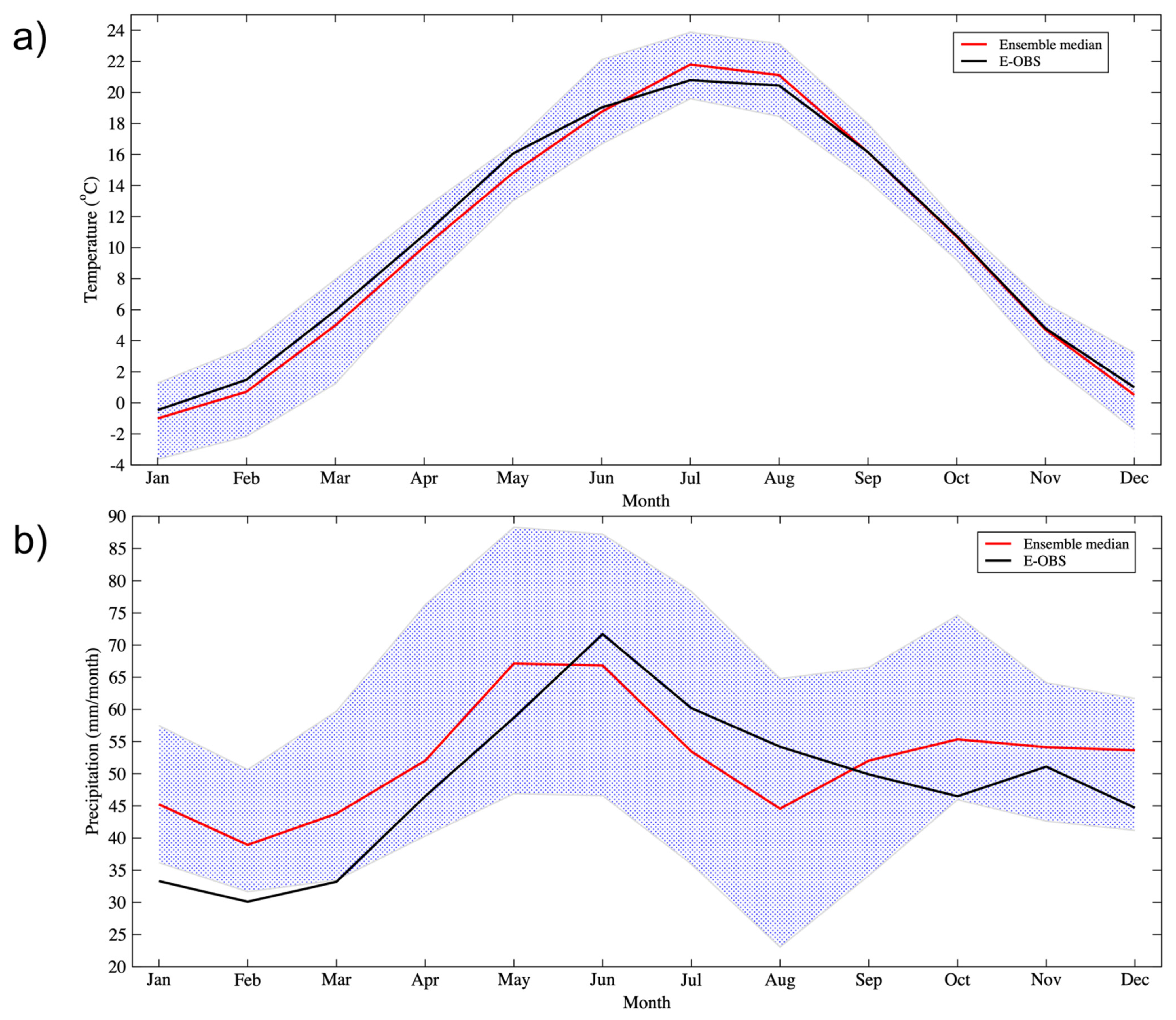
Before moving to the RCM data evaluation in terms of temperature and precipitation statistics, it is necessary to show the ability of RCMs to simulate climate characteristics, such as temperature and precipitation, during the year and over the region of interest. The annual cycles of monthly averaged mean temperature and monthly precipitation across the domain of the Pannonian Basin are depicted in
Figure 2. The data in
Figure 2 come from the E-OBS database, as well as the EURO-CORDEX RCM11 ensemble (0.11° grid). Across the Pannonian Basin, the temperature maximum is observed in July and August, while the temperature minimum is observed in December and January. Summer (June and July) brings the most precipitation to the Pannonian Basin, while winter (January and February) brings the least precipitation. The annual temperature cycle is mostly reproduced by the RCM ensemble median, with small departures from the E-OBS dataset with values up to 1 °C. The RCM ensemble median underestimates temperature in winter (December, January, February) and spring (March, April, and May), while overestimation is observed in summer (June, July, and August). In autumn (September, October, November), the ensemble temperature median coincides with the E-OBS dataset with the smallest spread of RCM simulations (area between the 5th percentile and 95th percentile). On the other hand, the RCM ensemble median underestimates precipitation in summer, while overestimation is present in all other seasons during the year. Notably, RCMs have the largest spread of their simulations in late spring (May) and summer when most convective processes occur in the Pannonian Basin, which indicates RCM uncertainty in representing precipitation during this part of the year.
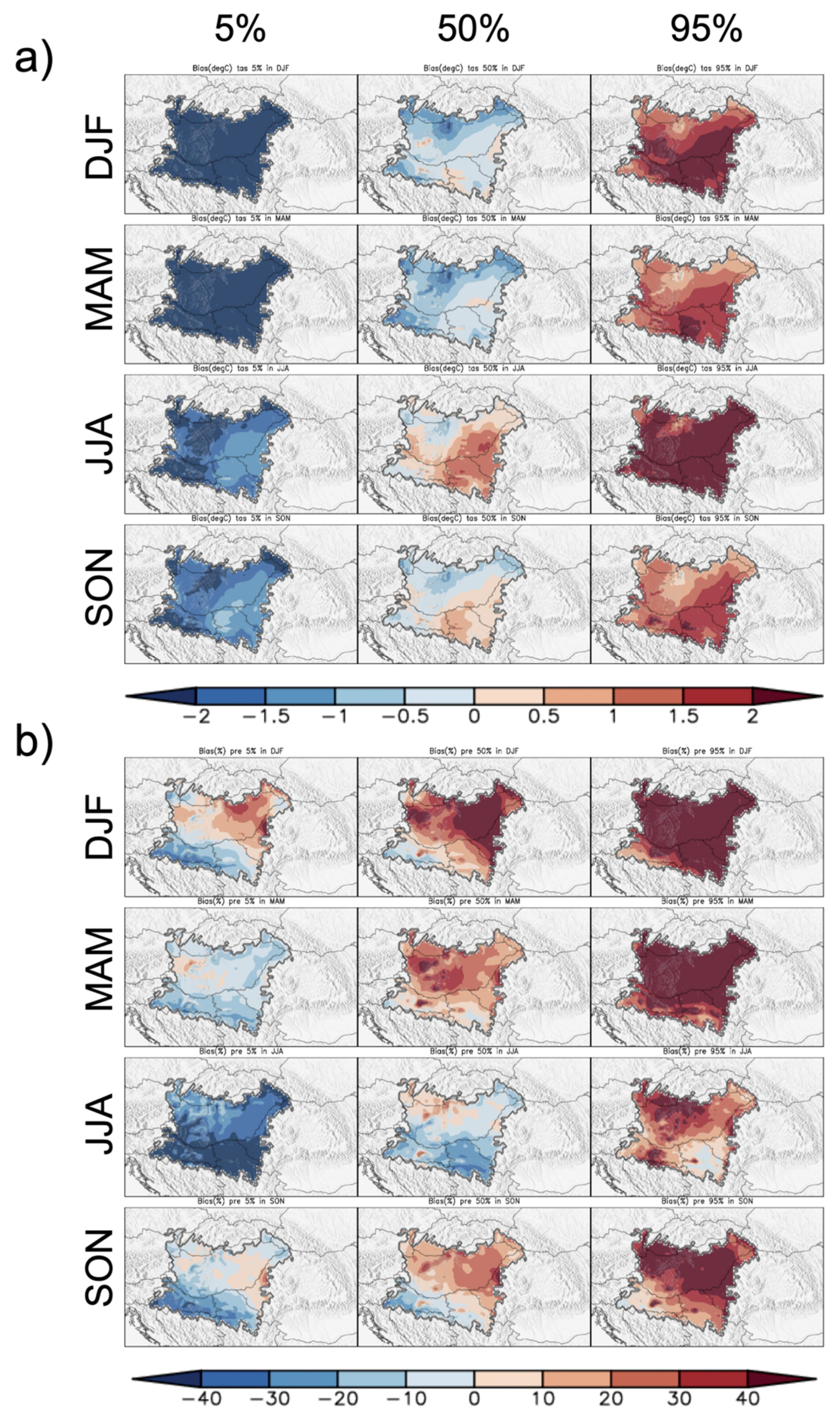
First, we investigated the ensemble overall temperature bias and precipitation bias. The 5th, median and 95th percentiles of temperature and precipitation biases among the 30 GCM–RCM simulations (cited in
Table 1) for all four seasons are shown in
Figure 3. These percentile maps indicate that not all models are biased in the same way, as we can see that the 5th percentile maps contain the most negative biases and the 95th percentile maps contain the most positive biases for temperature and precipitation biases. However, the exception is the winter season, where even the lower tail (5th percentile map) of the bias distribution is positive. This finding indicates that most RCMs tend to overestimate precipitation in winter (at least 95% of the RCMs have a positive bias).
According to the median of bias distribution, the most prominent feature in
Figure 3 is mostly widespread warm and dry bias during summer. The temperature median ranges from −1.2 to +1.6 °C, and the precipitation median ranges from −38% to +33%. The positive temperature and negative precipitation biases were even more pronounced for certain models, meaning the issue still exists in most examined simulations in the Pannonian Basin during the summer season. The upper tail of the temperature bias distribution (95th percentile map) is positive everywhere across the Pannonian Basin with biases up to 4 °C. The lower tail of the temperature bias distribution (5th percentile map) is negative everywhere with values below −2 °C in some parts, which indicates that some models tend to underestimate temperature. For the maximum and minimum temperatures, the same reveals that overall ensemble biases appeared in summer (not shown for shortness). On the other hand, the upper tail of the precipitation bias distribution (95th percentile map) is mainly positive across the Pannonian Basin with biases up to +70%. The lower tail of the precipitation bias distribution (5th percentile map) is negative everywhere, with values below −50% in some parts of the Pannonian Basin. Consequently, in this study, the main goal is to further examine in detail the existing summer drying issue in the Pannonian Basin and to inspect each individual RCM from the EURO-CORDEX multi-model ensemble.
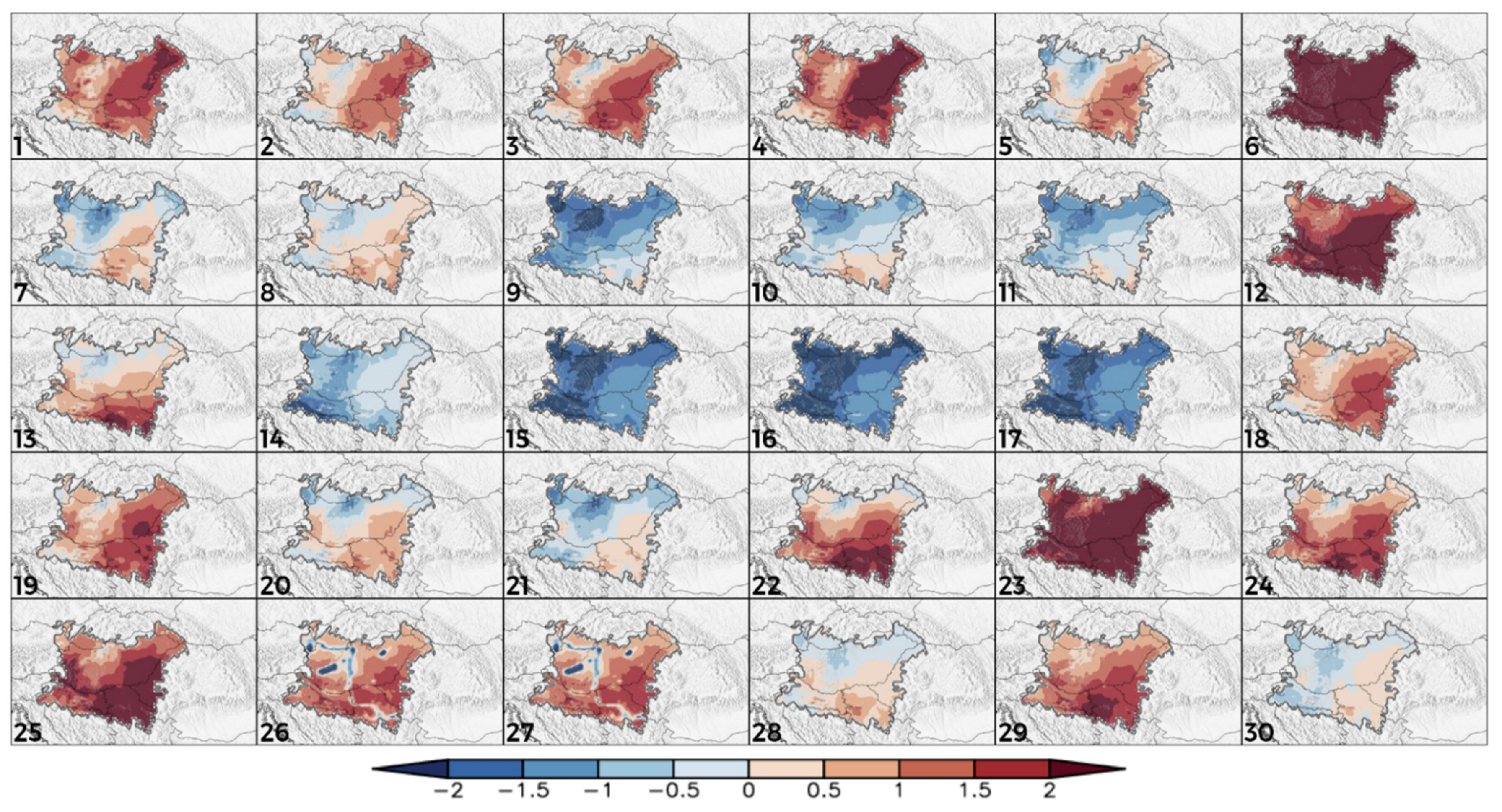
Figure 4 and
Figure 5 represent the spatial distribution of the mean (1971–2000) GCM–RCM bias for each individual model of the summer (June–July August, or JJA) mean temperature field and precipitation field, respectively, with respect to the E-OBS gridded dataset. Principally, there is spatial correspondence between temperature and precipitation biases, which is mostly pronounced during the summer as warm and dry biases in RCM simulations and, in a smaller number of cases, is reversed with cold and wet biases. This spatial correspondence is not visible in the ALADIN 5.3 simulation.
The same RCM is driven by different GCMs to examine the prevailing signal of positive or negative errors (with respect to representing mean temperature) of the corresponding driving models since GCM predominantly determines mean temperature bias [
38]. In
Figure 4 and
Figure 5, strong cold biases are found at a qualitative level, in summer, for the majority of RCMs downscalings in the EC-EARTH realizations (simulations denoted with numbers 9, 10, 11, 15, 16, 17, and 21), while HadGEM2-ES downscalings with different RCMs (simulations denoted with numbers 6, 12, 18, and 23) have the most pronounced warm and dry biases, which are straightforward in the sense that the overall biases presented in
Figure 6 and
Figure 7 are not a result of error cancelation. In
Figure 4, most RCMs driven with GCMs, such as CNRM-CM5 (simulations denoted with numbers 1, 2, 3, 4, and 19) and NCC-NorESM1-M (simulations denoted with numbers 13, 25, and 29), showed positive temperature bias; however, this warm bias was less pronounced than the warm bias present in HadGEM2-ES downscaling with different RCMs.
In support of the abovementioned fact, RCM HIRHAM 5 tends to underestimate summer temperature when forced by GCM EC-EARTH (denoted with numbers 9, 10, and 11), except for simulations denoted with numbers 8, 12, and 13 when driven with GCM CNRM-CM5 (warm bias). RCM RACMO 2.2E (simulations denoted with numbers 14, 15, 16, 17) maintains a strong negative temperature bias during the summer, except in the case when RACMO 2.2E is driven by GCM HadGEM2-ES (simulation denoted with number 18) since GCM HadGEM2-ES contributes as a warm bias. RCMs ALADIN 5.3 (denoted with number 1) and ALADIN 6.3 (denoted with number 2) were driven by the same GCM with features to overestimate the mean temperature, but ALADIN 5.3 (older version) had a greater positive temperature bias than ALADIN 6.3. Additionally, RCA 4 had a positive mean summer bias of temperature (denoted with numbers 19, 20, 22, 23, 24, and 25), excluding simulation when forced by GCM EC-EARTH (denoted with number 21), which showed cold temperature bias. RCM REMO 2009 (denoted with numbers 26 and 27) maintained a positive summer temperature bias. On the other hand, RCM REMO 2015 had the smallest temperature bias (simulations denoted with numbers 28 and 30), except in the case when it was driven by GCM NCC-NorESM1-M (marked with number 29) because of its positive warm bias contribution. Comparing the results among different RCMs forced by the same GCM when
Figure 4 and
Figure 6 are concerned, we concluded that RCM CCLM 4.8.17 forced by GCM HadGEM2-ES (denoted with number 6) had the greatest warm bias.
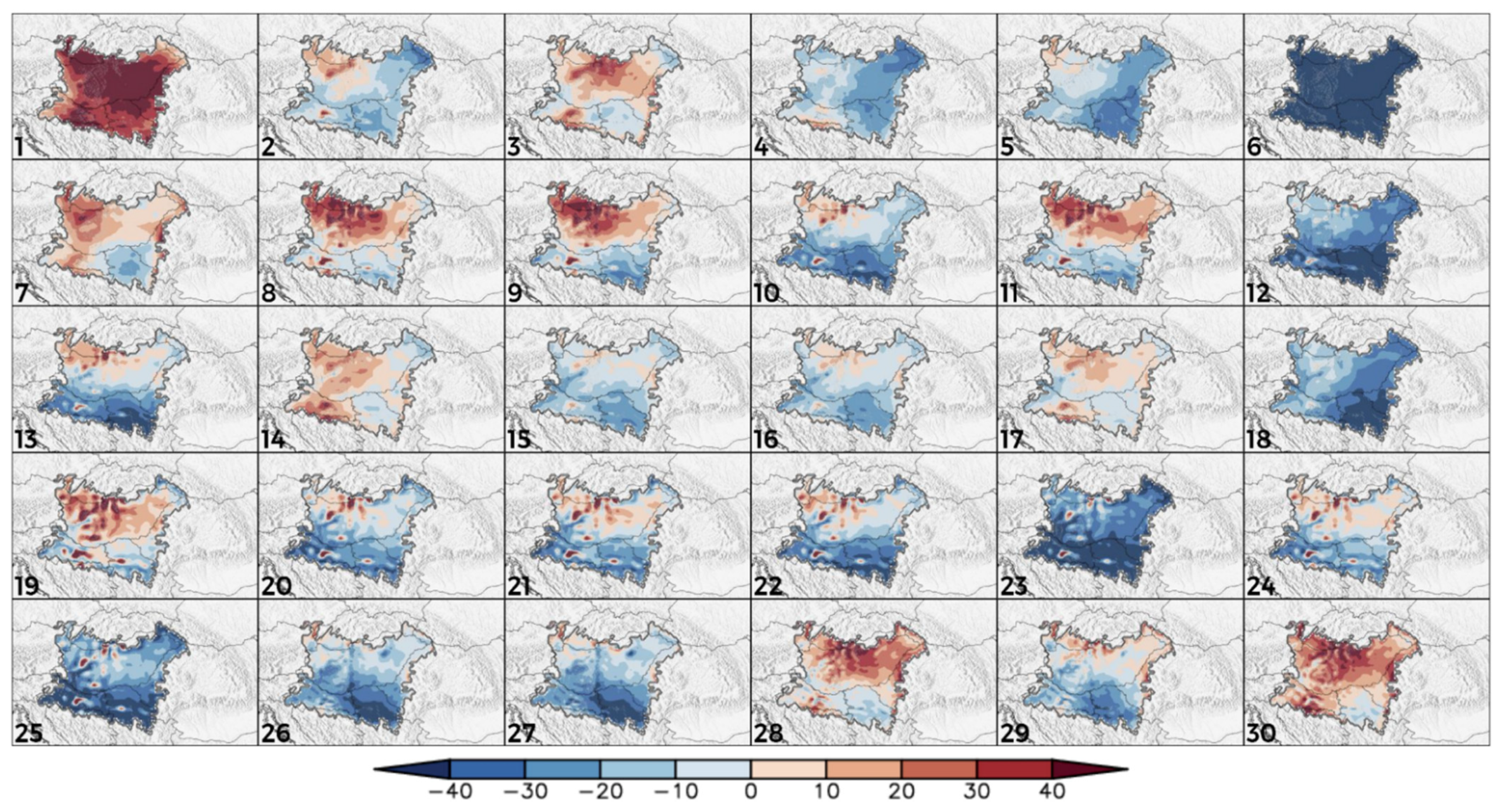
As mentioned, it is difficult to isolate the GCM and RCM contributions from the overall bias for precipitation due to the main drivers of precipitation, such as large-scale drivers and physical parameterizations, but some main and striking conclusions could be made.
Figure 5 shows that the previously specified downscaling of the HadGEM2-ES and NCC-NorESM1-M GCMs with different RCMs that overestimate temperature underestimates precipitation. In contrast, RCMs driven with GCM EC-EARTH tend to overestimate precipitation. RCM ALADIN 5.3 has an issue with representing precipitation due to its overestimation, although ALADIN 5.3 also overestimates the mean temperature. However, spatial correspondence between temperature and precipitation bias is observed in RCM ALADIN 6.3, which is driven with the same GCM as ALADIN 5.3. Additionally, RCM CCLM 4.8.17 tends to underestimate precipitation.
These results obtained from
Figure 4 and
Figure 5 correspond with the results from Reference [
38] for the Eastern Europe region where GCM and RCM contributing biases are examined, except that in the Pannonian Basin, temperature bias was even more emphasized for certain GCM–RCM combinations.
Note that the E-OBS reference dataset errors are larger in the summer season for the precipitation field since summer precipitation is mainly convective rather than frontal [
38,
44]. Hence, verification of the precipitation field with respect to E-OBS has more uncertainty than temperature validations. In addition, as observed in Reference [
38], RCMs tend to overestimate precipitation in summer more than in winter due to the E-OBS deficiency in the present observed precipitation field. Hence, we assume that summer precipitation underestimation over the Pannonian Basin is even more pronounced because E-OBS underestimates summer precipitation.
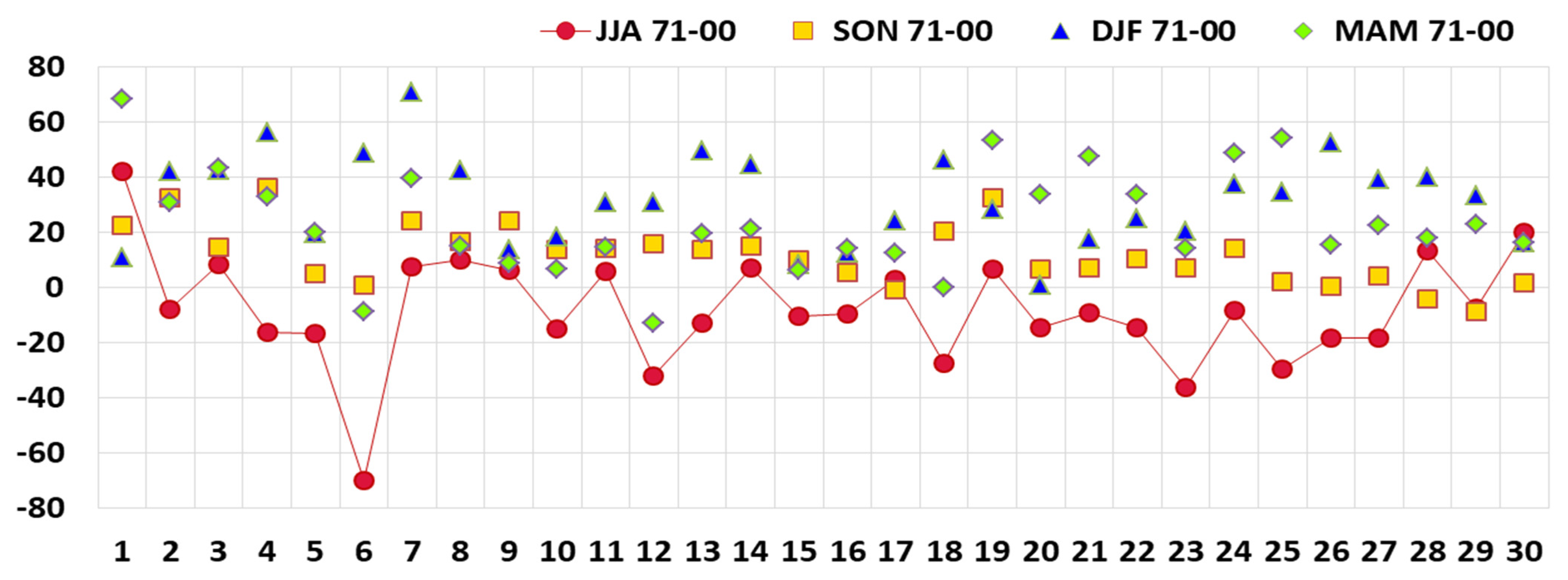
The different parameterizations used in the analyzed RCM simulations or transportable error from GCMs used for downscaling are directly responsible for the broad range of examined GCM–RCM seasonal biases, as we can see in
Figure 6 and
Figure 7. Temperature and precipitation biases do not remain constant during seasons for a particular GCM–RCM combination, so
Figure 6 and
Figure 7 indicate a strong time dependence. However, the annual cycle is seen in
Figure 6, where most RCMs overestimate summer temperature. According to our findings, in
Figure 6 and
Figure 7, where spatially averaged overall bias is presented, 17 RCMs overestimate temperature, 8 RCMs underestimate temperature, and 5 RCMs estimate temperature around the E-OBS gridded dataset during the summer season. Most RCMs that overestimate temperature, on the other hand, underestimate precipitation during the summer season. The summer temperature bias ranged from −1.9 to +4.4 °C, while the summer precipitation bias ranged from +42% to −70%.
Note that in some cases, the near-zero overall mean temperature biases (5 RCMs) presented in
Figure 6 and
Figure 7 are a result of error cancelations, as seen in
Figure 4 and
Figure 5. For instance, CCLM4–8-17 driven by MPI-ESM-LR (listed as number 7), HIRHAM 5 driven by CNRM-CM5 (listed as number 8), RCA4 driven by EC-EARTH (listed as number 20), REMO 2015 driven by IPSL-CM5A-LR (listed as number 28) and NOAA-GFDL-GFDL-ESM2G (listed as number 30) approximately did not show overall summer temperature bias in
Figure 6, but we can see the bias in
Figure 4.
To examine the “summer drying” issue over the Pannonian Basin in more detail, additional assessments are carried out over a selected subregion in the Carpathian region (Pannonian Basin). In this study, the main goal was to statistically examine the ability of RCMs to represent temperature and precipitation fields in the summer season. The other three seasons are displayed for comparison only.
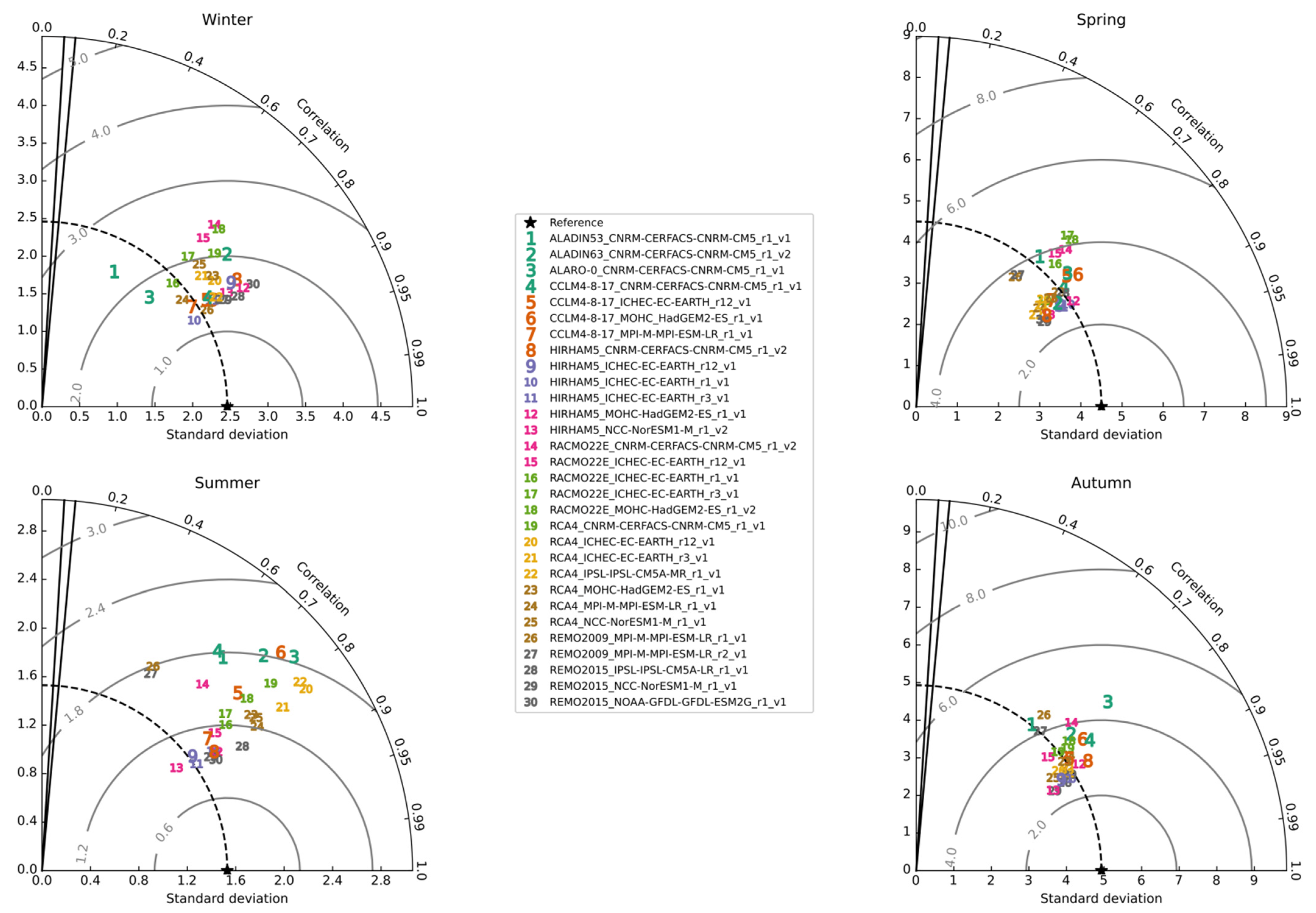
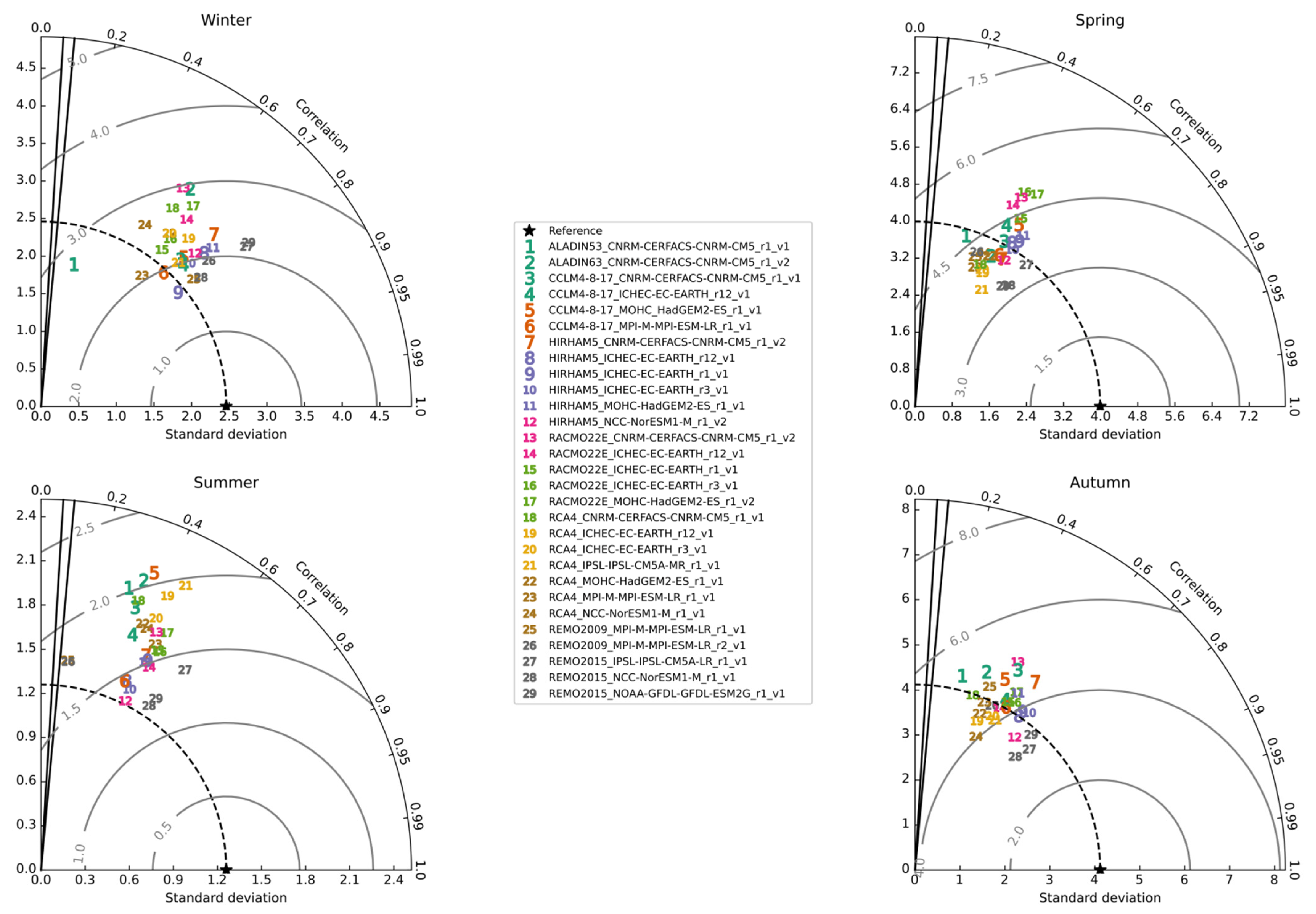
Three statistics, such as centered RMSE along with the standard deviations and the spatial correlations of RCM simulations of four meteorological variables (tas, tasmax, tasmin, and pre), were assessed against the E-OBS dataset over the Pannonian Basin for the 1971–2000 period in
Figure 8,
Figure 9,
Figure 10 and
Figure 11. Statistics are calculated over all 2205 grid cells of the observed field and from the thirty GCM–RCM simulations, except for tasmax and tasmin, where twenty-nine simulations were available and evaluated. The Taylor diagrams enable us to graphically indicate the individual RCM that is the most realistic compared with the E-OBS dataset. In
Figure 8,
Figure 9,
Figure 10 and
Figure 11, where Taylor diagrams are presented, there is a table that displays a list of evaluated GCM–RCM simulations. In the table, simulations are divided into four parts by an underscore. The first section represents the name of the RCM driven by the GCM determined in the second section, the third section shows the identified realization of the same GCM driver, and the fourth section shows the RCM version.
From
Figure 8,
Figure 9,
Figure 10 and
Figure 11, we notice that for the summer season, the presented scores show the highest spatial variability in comparison to the other three seasons for all examined variables (tas, tasmax, tasmin, and pre), which represent EURO-CORDEX model uncertainty in simulating meteorological fields, as well as disagreement in standard deviation compared with the observed field. This main feature is present to the greatest extent in models’ performance to represent tasmax during summer. If we consider temperature variables (tas, tasmax, and tasmin), the spatial correlation coefficients are the lowest in the model performance to simulate tasmin fields in all seasons (especially in summer). According to [
38], this finding could indicate that RCM biases mainly contribute to the overall bias in this case due to deficiency in local physical parameterizations. The lowest spatial correlation coefficients among all four examined fields (tas, tasmax, tasmin, and pre) are noticeable in precipitation fields. On the other hand, the spatial correlation coefficients are the highest in the model performance to simulate tasmax fields. The models overestimate spatial variability in summer (standard deviations of most model fields are constantly high in comparison to the observed field, especially for tas and tasmin), indicating that the models produce wider distributions. Moreover, different realizations of the same GCM driver used to estimate the impact of simulated natural variability on climate change responses do not show significantly different Taylor statistics for the same GCM.
According to
Figure 8, grid cell correlations for the mean temperature field are also relatively lower in summer than in the other three seasons, and the spread of correlations ranges between 0.48 and 0.85. Summer correlation coefficients are high in general (most RCMs have correlation coefficients between 0.71 and 0.85). Furthermore, during the summer, in contrast with observations, RCM REMO 2009, with a slightly overestimated standard deviation, had the lowest performance in terms of the spatial correlation coefficient (approximately 0.48) and centered RMSE. In agreement with
Figure 4 and
Figure 6, REMO 2009 had a slightly wider shifted temperature distribution toward higher values addressed as large positive bias and the largest standard deviation of the model error (centered RMSE), which indicates model inaccuracy. Notably, HIRHAM 5 and REMO 2015 are among the best-performing RCMs (correlation coefficients are high at >0.8), especially during the summer, conforming to the Taylor diagram in
Figure 8. However, this result does not mean that a temperature bias does not exist in these simulations, as shown in
Figure 4. In addition, RCM RCA 4 driven by different GCMs had high spatial correlation coefficients despite the overestimated standard deviations compared with the E-OBS dataset and high centered RMSE during summer. RCM RCA4 showed this common pattern in all three Taylor diagrams where temperature statistics are presented (tas, tasmax, and tasmin).
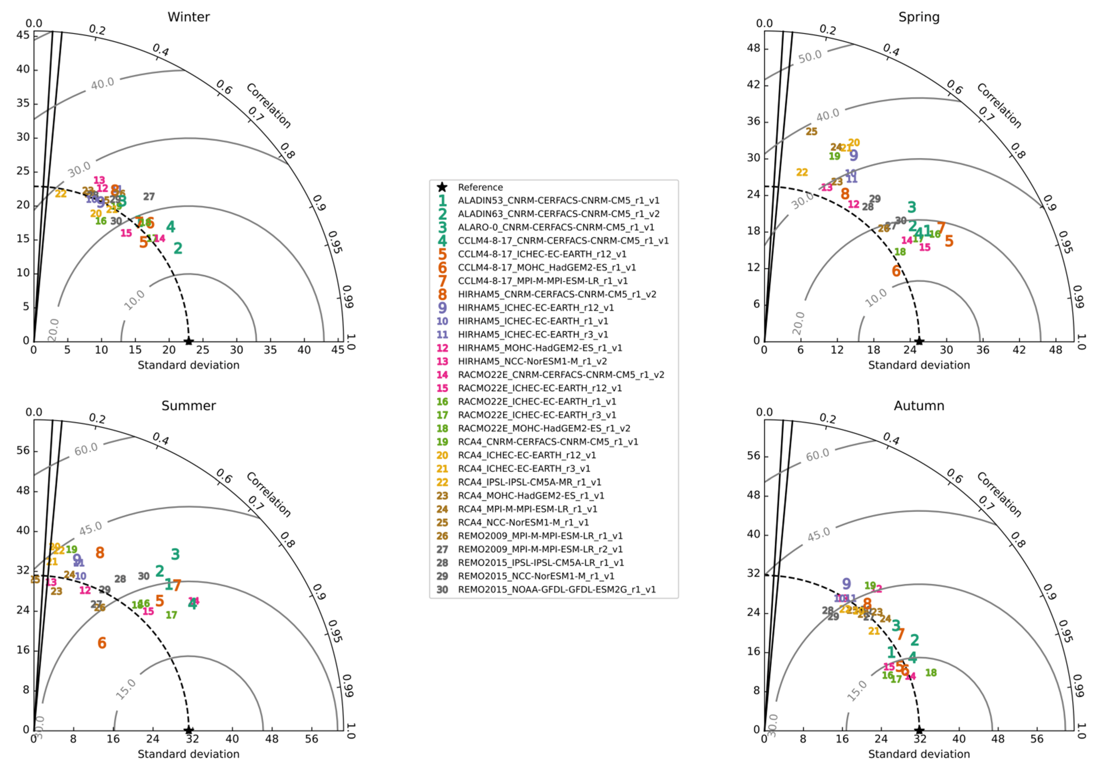
RCM simulations for precipitation (
Figure 9), in comparison to temperatures (
Figure 8,
Figure 10, and
Figure 11), indicate lower compliance with observed fields (<0.8 in all cases). Spatial precipitation correlation values for GCM–RCM combinations are much lower than those for temperatures (tas, tasmin, and tasmax) and in some cases are not statistically significant (RCA4 driven by NCC-NorESM1-M numbered 25 in
Figure 9). The spread of spatial correlations ranges between close to 0 and 0.78. During winter and autumn, the best compliance with the observed field was observed when all three statistics presented in the Taylor diagram were considered. This finding is in accordance with previous research that suggests that climate models simulate stratiform synoptic-scale precipitation better than local convective precipitation [
55].
According to the Taylor diagram in
Figure 9, RCMs such as RACMO 2.2E and CCLM 4.8.17 showed the best performance in representing the precipitation field with spatial correlation coefficients higher than 0.6, although in
Figure 5, these RCMs had a nonzero bias. These RCMs have a mostly wider precipitation distribution toward lower values, which is addressed as a large negative bias and the lowest standard deviation of model error (centered RMSE). The RCMs with the lowest score were RCA 4 with spatial correlation coefficients lower than 0.2. These findings are consistent with previous work for the Carpathian region [
49]. Additionally, even though RCMs REMO 2015 and HIRHAM 5 showed the best performance according to the temperature verification, these RCMs realized lesser performances with spatial correlation coefficients lower than 0.6 with respect to the evaluation precipitation field. REMO 2015 is slightly better than HIRHAM 5 according to the three precipitation statistics displayed in
Figure 9.
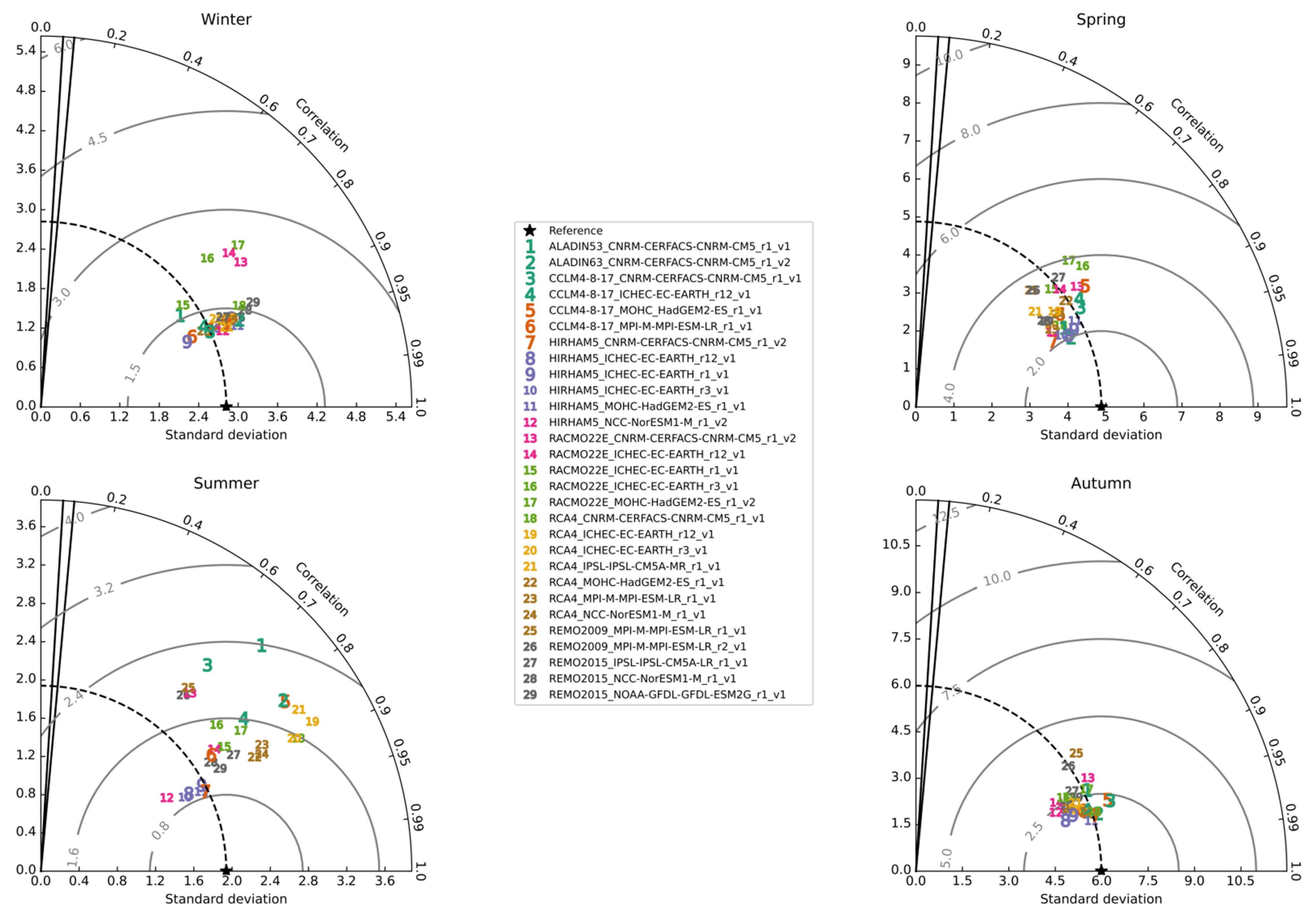
According to
Figure 10, similar RCM performances are observed in representing tasmax as those representing tas during the summer. The main difference is that RCMs showed the highest spatial variability during summer in comparison with the other three seasons in representing the maximum temperature field. This result is because HIRHAM 5 underestimates the standard deviation compared with the observed field, while other RCMs overestimate the standard deviations. During summer, the spread of correlations is between 0.62 and 0.90, reflecting the highest correlations among the other three variables (tas, tasmin, and pre). The correlation coefficients in summer are generally high (most RCMs have correlation coefficients between 0.76 and 0.89). The best-performing RCMs during summer are REMO 2015 and HIRHAM 5, with spatial correlation coefficients higher than 0.85 and with slightly more enhanced performances to represent tasmax than representing tas. Generally, RCMs have better statistical scores in representing tasmax than tas in summer. On the other hand, REMO 2009 has poorer scores, as was the case with tas. In line with
Figure 10, the lesser performances in summer are from RCMs ALADIN 5.3 and CCLM 4.8.17 driven by CNRM-CM5. RCM ALADIN 6.3 realized a better performance with respect to the Taylor statistics than RCM ALADIN 5.3.
Figure 11 shows that the RCM performances for tasmin fields in the summer season are worse than the performances for tas and tasmax with regard to all three statistics, especially concerning a spatial correlation coefficient. During summer, the spread of correlations is between 0.12 and 0.58. RCM REMO 2009 had the lowest scores (the highest RMSE values) in representing tasmin due to the largest centered RMSE and the lowest spatial correlation coefficient (0.12). RCMs REMO 2015 are among the top models in representing tasmin, with a spatial correlation coefficient of approximately 0.5.
Finally, as an additional metric of the model performance, we examined the temperature trend over the period of 1970–2005. The results from
Table 2 show that RCMs had a positive trend in the observed field for the last 36 years (only RCM HIRHAM 5 driven by GCM NCC-NorESM1-M did not show either positive or negative trends). The RCMs that showed the smallest departure from the observed temperature trend were ALADIN 5.3, CCLM 4.8.17 driven by EC-EARTH r12 and HadGEM2-ES, HIRHAM 5 driven by HadGEM2-ES, RACMO 2.2E driven by EC-EARTH r12, RCA 4 driven by MPI-ESM-LR, and REMO 2015 driven by NCC-NorESM1-M and NOAA-GFDL-GFDL-ESM2G. The temperature trends and temperature summer bias do not seem to be connected, which means that warm/cold summer temperature bias does not indicate overestimated/underestimated temperature trends compared with the E-OBS dataset and reverse.
4. Conclusions
RCMs are valuable sources of fine-scale climate information because they are often used as input to assess the impact of possible climate change in the future on certain socioeconomic sectors of society or the environment. The main goal of the present study was to test whether dry and warm biases existed in summer over the Pannonian Basin in thirty RCM simulations of the EURO-CORDEX initiative, as was the case in previously mentioned studies and projects of dynamic downscaling across Southeastern Europe. All verification scores in this paper are evaluated for the domain of the Pannonian Basin and for temperature and precipitation fields. According to our GCM–RCM evaluation, we conclude that none of the GCM–RCM pairs are improbable. On the other hand, the ensemble has systematic biases, and the simulations have common deviations from observations. Our results confirmed that, in summer, in many different RCM simulations, dry and warm biases were detected across the Pannonian Basin; however, few RCMs showed cold and wet biases. The median of the simulations is hotter and drier than that observed in the Pannonian Basin during the summer, with the widest RCM simulation distribution. Furthermore, we observed that, for all examined variables (tas, tasmax, tasmin, and pre), verification scores in the summer season displayed the highest spatial variability in comparison to the other three seasons, which represents EURO-CORDEX model uncertainty in simulating meteorological fields.
Generally, determining the best or worst GCM–RCM pair is futile because the skills are highly dependent on the area and examined meteorological field. However, in this study, we limited ourselves to the area of the Pannonian Basin. The RCM that stands out with good scores in simulating temperature fields is REMO 2015; and, on the other hand, good performance in representing the precipitation field showed RACMO 2.2E and CCLM 4.8.17. In conclusion, RCMs with good performances in representing temperatures do not necessarily perform well in representing precipitation, and vice versa. In general, and considering only temperatures, RCMs have the best statistical scores representing maximum temperature and the worst statistical scores in representing minimum temperature. However, the same RCM driven by certain GCMs showed similar tendencies in representing all three temperature fields (tas, tasmax, and tasmin). On the other hand, the lowest spatial correlation coefficients among all four examined fields (tas, tasmax, tasmin, and pre) were present in precipitation fields. However, most RCMs that overestimate temperature also underestimate precipitation.
Hence, one of the possible reason for the observed summer drying problem may be in representation interaction and feedback between soil moisture (land) and atmosphere and, for instance, in the false representation of soil type [
28]. As mentioned before, soil type defines parameters that have a major impact on soil moisture conditions and surface fluxes. Soil moisture is an essential feature of the land–atmosphere interaction that affects the conditions on the surface, such as radiation and humidity [
28]. Therefore, our next goal in further researches is to examine the soil moisture—atmosphere interactions in RCM in the Pannonian Basin (such as investigating annual cycle of soil moisture for soil layers after changing the soil type, comparing RCM soil moisture data with observed data, etc.) in order to reduce to some extent warm and dry bias. It is important to note that according to a former study [
56], it is found that one of the primary sources and trigger for dry and warm bias in the summer season is precipitation deficit regarding the fact that local and small-scale convection systems are not captured well in RCMs. Precipitation deficit thereafter is followed by complex land–atmosphere interactions that cause the positive bias in temperature fields. Initial intention in this paper was to check if high-resolution runs (that were not available in the past) helped in terms of negative precipitation and positive temperature bias in the region, in the first place by better representation of convective precipitation during the summer. Our hypothesis was that higher resolution will lead to more localized and higher convective precipitation (a common feature of the models) that can reduce some of the biases. To our surprise, some of the models, even though they have run in high-resolution mode, still produce similar errors, as low-resolution ones (comparing with previously published research on this topic). We found this very interesting as proof that higher resolution is not simply a solution to some ‘old well-known biases’. Consequently, to better understand the sources and reasons for the summer drying problem to improve the ability of RCMs to represent the past climate in the Pannonian Basin, further research is needed. The results from the driving GCMs should also be verified to determine the effect of various lateral boundary conditions on the results from RCM simulations and to examine the added value of downscaling more thoroughly in RCMs.


