Heating and Cooling Degree-Days Climate Change Projections for Portugal

Abstract

Climate change is expected to influence cooling and heating energy demand of residential buildings and affect overall thermal comfort. Towards this end, the heating (HDD) and cooling (CDD) degree-days along with HDD + CDD were computed from an ensemble of seven high-resolution bias-corrected simulations attained from EURO-CORDEX under two Representative Concentration Pathways (RCP4.5 and RCP8.5). These three indicators were analyzed for 1971–2000 (from E-OBS) and 2011–2040, and 2041–2070, under both RCPs. Results predict a decrease in HDDs most significant under RCP8.5. Conversely, it is projected an increase of CDD values for both scenarios. The decrease in HDDs is projected to be higher than the increase in CDDs hinting to an increase in the energy demand to cool internal environments in Portugal. Statistically significant linear CDD trends were only found for 2041–2070 under RCP4.5. Towards 2070, higher(lower) CDD (HDD and HDD + CDD) anomaly amplitudes are depicted, mainly under RCP8.5. Within the five NUTS II regions projections revealed for 2041–2070 a decrease in heating requirements for Algarve and Lisbon Area higher in Faro, Lisboa and Setúbal whereas for North and Center regions results predicts an increase in cooling energy demand mainly in Bragança, Vila Real, Braga, Viana do Castelo, Porto and Guarda, higher under RCP8.5.

1. Introduction

Climate changes have a profound impact on natural [1] and human systems. The projected impacts of 1.5 °C global warming [2,3] will increase the intensity and frequency of some climatic and extreme weather events [4,5], which in turn will result in negative impacts on resources, biodiversity, and ecosystems [6].

Several regions are most vulnerable to these projected changes; this is the Mediterranean region’s case [2,7], including southern Europe in which Portugal is included. Since exposure to multiple and compound climate-related risks is projected to increase, assessing its impacts on human systems is highly relevant.

The projected rise in temperatures [8] is expected to pose greater risks to urban areas. The extent of the risk depends on human vulnerability (for example, elder citizens are more vulnerable to higher temperatures) and adaptation effectiveness, namely in the construction sector. Household residences are of special concern since about 65% of the time is spent inside residences; therefore, deviations in thermal comfort conditions can have detrimental impacts in citizens, as previously mentioned elders and also children who spend more than 90% of the time indoors [9]. The fluctuations in outdoor air temperatures [10] will have not only a substantial impact on human comfort, but also on building energy use [11] mainly in the existing residential buildings. Therefore, estimated air temperature fluctuation projections have relevant implications for estimating its future impacts on residential heating and cooling related energy demand.

Several studies used multiple methods to estimate future residential heating and cooling energy demand in buildings. While some authors choose simple approaches such as using current climate, discarding climate variability [12] or choosing a warm past year to represent a warming climate [13], others opt to use climate models using several datasets, namely global climate simulation models (GCMs) [11,14,15,16,17,18,19]. The most common methods used to determine residential demand in the future use parametric energy balance and degree-day methods. The degree-day method is a simple and widely used approach to relate outdoor temperature with the heating/cooling energy requirements.

In this study, we employed the degree-day method following the procedure used by Petri and Caldeira [16] and, later, by Spinoni et al. [11]. This methodology defines a base temperature (Tb) for the heating and cooling season and allows the computation of the respective outdoor air temperature deviations from maximum and minimum temperatures. The base temperature is a point at which internal gains equal the heat loss, acting as a threshold below (or above) which heating (or cooling) appliances are needed or not to operate to maintain indoor thermal comfort. Under the Portuguese Regulation on the Energy Performance of Residential Buildings (REPRS) [20,21], these temperatures are 18 °C related to the degrees-day of heating (HDD) and 25 °C to the degrees-day of cooling (CDD). Further details will be provided in the Materials and Methods section; however, it is worth mentioning that the REPRS is in line with the European Directive 2010/31/EC [22], which aims at reducing the greenhouse gas emissions by 20% by 2020 and in 80% until 2050, in relation to the 1990 emissions levels. Therefore, this objective includes the adoption of standard methodologies for calculating energy consumption, quality requirements for new and existing building envelopes, periodic inspection of boilers and air conditioning central systems, as well as building energy certification.

Three key energy performance indicators were computed in this work: the HDD, the CDD and the global indicator HDD + CDD, obtained from an ensemble mean of seven biased corrected regional climate models (RCMs) for mainland Portugal. Three-time periods were analyzed: 1971–2000 (the historical baseline climate), 2011–2040 and 2041–2070. For the latter periods, two representative concentration pathways (RCPs) were considered: a mitigated scenario RCP4.5 and the RCP8.5 unmitigated climate scenario [2]. For the trend analysis, 2011–2070 period is also assessed along with 2041–2070 and the entire period comprised between 1971 and 2070.

Typically, the data from ground stations are interpolated to estimate meteorological characteristics over larger regions. Spatial interpolation makes it possible to estimate any meteorological characteristic at locations away from those for which direct measurements exist. Inverse distance weighted (IDW), ordinary kriging (OK), and ordinary cokriging (OCK) are the most frequently used techniques in environmental studies for spatial interpolation of data [23,24,25,26,27,28]. Several geostatistical techniques were performed in this study to attain the most accurate spatial representation of the different indicators.

This study’s main goal is to analyze the impacts of climate change on heating or cooling related energy demand for residential buildings thermal comfort by computing HDD, CDD and HDD + CDD for five regions of the Nomenclature of Territorial Units for Statistics (NUTS) NUTS II of mainland Portugal (Figure 1). The results presented herein under RCP4.5 and RCP8.5 until 2070 will serve as an indicator of projected climate change and help policymakers improve laws that lead to more sustainable construction techniques in terms of mitigation and adaptation. Architects and building engineers can no longer assume a constant static condition for their designs and need to consider the values of design variables for future years.

2. Materials and Methods

The overall methodology framework can be depicted in Figure 2 but will be detailed in the following subsections.

2.1. Study Area

The study area of interest is the five NUTS II regions of mainland Portugal: North, Center, Lisbon Metropolitan Area, Alentejo and Algarve (Figure 1). Besides assessing HDD, CDD and HDD + CDD for Portugal, the second objective of this study is to analyze climate change’s impacts in each NUTS II region. This territory has the two largest urban areas in the country, Lisbon Metropolitan Area, with a population of 2,821,876 inhabitants (28% of the total Portuguese population) [29] and the urban area of Porto in the North, with over 1,700,000 inhabitants (17% of the total Portuguese population) [30].

The Shuttle Radar Topography (SRTM) mission explored the structure of the earth surface from which SRTM-3 with a resolution of three arc seconds (about 90 m) was retrieved. The elevation in mainland Portugal varies from 0 m (near the Atlantic Ocean) to 1993 m (in the Estrela Mountain, located in the center-eastern) with a mean elevation of 323 m above mean sea level. Less than one-eighth of Portugal rises above 700 m. Portugal and Spain share their major rivers—Douro, Tagus, Guadiana—rise in the central Meseta before draining west (or, in the case of the Guadiana, south) to the Atlantic. The North and Center of the country are mountainous with elevations up to 1544 m (Gerês). In the North of the northern interior region are high plateaus at 600–800 m. Between the Douro and the Tagus rivers lies the central mountain range with the Serra da Estrela (1993 m in the Torre, the highest point in continental Portugal), North of the Tagus river, more than nine-tenths of the land rises above 400 m. Some three-fifths of Portugal’s land below 400 m are found in the south. In Alentejo, the S. Mamede mountain range (1027 m) and in the Algarve, the Monchique mountain range (902 m) is noteworthy. Portugal has more than 800 km of coastline, four-fifths of which faces westward.

Most of Portugal has a warm Mediterranean climate, according to the Köppen climate classification: Hot-summer Mediterranean climate (CSa) and Warm-summer Mediterranean climate (CSb). A small region in inland Alentejo has Cold semiarid climate (BSk). South of Serra da Estrela, there are high temperatures in summer and cool winters, with dry summers and wet winters [31]. Towards the North of Serra da Estrela, in the north-east portion of the country, the effect of continentality versus oceanity contrasts are more pronounced, e.g., more humidity along with lower average temperatures, especially in the high-altitude areas, while in the lower, such as the Douro Valley, high values, similar to those in the south of the country are registered. In the North Coast (in the Northwest of the country), the climate is Mediterranean with a maritime influence and has moderate summers.

Average annual temperatures in mainland Portugal range from 18 °C in Faro to 10 °C in Guarda, the country’s highest and coldest city, while rainfall varies from less than 500 mm in southern parts of Alentejo to over 3000 mm in the Serra do Gerês. The country’s coldest place is Serra da Estrela, which has an average annual temperature of 7 °C in the highest parts. Nevertheless, there is considerable climatic variability from one year to the next.

The population distribution within Portugal reveals contrasts between the more densely populated North and the more sparsely populated south. With their low-lying plains and urban development, the coastal zones between Oporto and Lisboa have attracted many populations. Overall, 43.7% of Portugal’s population live in urban areas in Área Metropolitana de Lisboa, Centro and Norte NUTS II regions.

2.2. Datasets and Bias Correction

In this study, E-OBS maximum and minimum temperatures gridded observational datasets were retrieved from EU-FP6 project UERRA (http://www.uerra.eu, accessed on 20 December 2020) and the data providers in the ECA&D project (http://www.ecad.eu, accessed on 20 December 2020), for the period between January 1971 to December 2017) [32]. The daily mean, maximum and minimum temperature (Tx and Tn, °C) datasets are defined on a 0.25° regular grid.

Maximum and minimum temperatures daily projections for the period between 1971–2005 (historical) and 2006–2070 were taken from the EURO-CORDEX initiative (http://www.euro-cordex.net/, accessed on 20 december 2020) that provides regional climate projections for Europe at 12.5 km (EUR-11) resolution. The Coupled Model Intercomparison Project 5 (CMIP5) global climate projections [33] provided these new regional simulations in the RCPs [34,35], in this case under RCP4.5 and RCP8.5. The RCP8.5 can be interpreted as a rising radiative forcing pathway leading to 8.5 W/m² in 2100 [36,37], whilst RCP4.5 implies a stabilization without overshoot pathway to a 4.5 W/m² stabilization after 2100 [38,39,40]. In this study, seven RCMs were retrieved from EURO-CORDEX (

Table 1. Acronyms of the Regional Climate Models (RCM) and corresponding driving models.

Contributor	Driving Model	RCM
Météo France, CNRM	CNRM-CM5	ALADIN53
Royal Meteorological Institute of Belgium and Ghent University, RMIB	CNRM-CM5	ALARO-0
Climate Limited-area Modelling Community, CLMcom	ICHEC-EC-EARTH	CCLM4-8-17
Danish Meteorological Institute, DMI	ICHEC-EC-EARTH	HIRHAM5
Royal Netherlands Meteorological Institute, KNMI	ICHEC-EC-EARTH	RACMO22E
Max Planck Institute for Meteorology, MPI-CSC	MPI-ESM-LR	REMO2009
Institute Pierre-Simon Laplace, IPSL-INERIS	IPSL-CM5A-MR	WRF331F

). Let us remind that the use of RCMs generated by climate models has several uncertainties henceforth affecting their ability to accurately simulate changes in the complex climatic system. Therefore, there are differences between observations and raw climate model outputs. As a result, a bias correction towards the observed climatology is needed. Spinoni et al. [11] also addressed the uncertainty by computing the relative standard error of ensemble mean of the trend values. It was concluded that for Europe, the relative standard error is smaller under RCP8.5 than RCP4.5 and rarely have exceeded 0.1 for both HDD and CDD. Spinoni et al. [11] also pointed out that this is due to smaller intermodel variability under RCP8.5, whereas under RCP4.5 the agreement between simulations is less clear. Either for HDD or CDD no noticeable uncertainties were pointed out to Portugal [11].

The observational data was extended by GCM projections, covering a period between 1971 and 2070. Bias correction was applied to the original variable’s simulations using the observational data as a baseline climate (1971–2000) referred to as ‘obs, control’ in Figure 3. The E-OBS datasets and the respective GCMs that have a coarser spatial resolution on 0.11° regular grid overlap thus allowing this bias correction. In this study, we used the quantile-quantile bias correction. This method assumes that the distribution function of a variable may change in the future. However, this methodology allows the correction of the complete distribution, tails included. Further details regarding this methodology can be found in Viceto et al. [5]. Bias correction was applied to daily mean, minimum (Figure 3a) and maximum temperatures (Figure 3b) for the entire study region. Figure 3 shows the respective cumulative distribution functions (CDFs) represented by the application of this bias correction methodology for the historical period (1971–2000), for both Tx and Tn, by projecting the distribution of the observed Tx and Tn (obs, control) onto the simulated Tx and Tn (RCM, control). Afterwards, Tx and Tn are biased corrected for all periods (RCM, cor). All variables were biased corrected, and an ensemble-mean of seven state-of-the-art RCMs (Table 1) was used to compute the HDD and the CDD.

2.3. Heating (HDD) and Cooling (CDD) Degree-Day

Energy consumption linked to the thermal comfort of buildings is related to the HDD and the CDD. The HDD translates the amount of energy needed (i.e., to a building with a heating system) on a given day or period to heat the indoor environment in a climate considered cold to a specific base temperature (18 °C). The CDD reflects the amount of energy required (i.e., for a building with a cooling system) on a given day or period to cool the indoor environment in a climate considered warm to a specific base temperature (25 °C). The theoretical formulation for calculating the HDD (in °C × D per year) and CDD (in °C × D per year) can be carried out in several ways. Calculations can be performed using monthly or annual data or with more sophisticated models. Although the base temperature values may differ, depending on the country under analysis, in this work, the daily values for the HDD should be determined using a base temperature (Tb in

Table 2. Calculation of daily HDD values by comparing the maximum and minimum temperatures relative to the base temperature (Tb) [11,16].

Case	Condition	HDD
1	$Tx\le Tb$	$HDD=Tb-Ta$
2	$Ta\le Tb<Tx$	$HDD=\frac{Tb-Tn}{2}-\frac{Tx-Tb}{4}$
3	$Tn<Tb<Ta$	$HDD=\frac{Tb-Tn}{24}$
4	$Tn\ge Tb$	$HDD=0$ (no need to heat)

) of 18 °C, while the daily CDD values using a base temperature (Tb in

Table 3. Calculation of daily CDD values by comparing the maximum and minimum temperatures relative to the base temperature (Tb) [11,16].

Case	Condition	CDD
1	$Tx\le Tb$	$CDD=0$ (no need to cool)
2	$Ta\le Tb<Tx$	$CDD=\frac{Tx-Tb}{4}$
3	$Tn<Tb<Ta$	$CDD=\frac{Tx-Tb}{2}-\frac{Tb-Tn}{4}$
4	$Tn\ge Tb$	$CDD=Ta-Tb$

) of 25°C [20,21]. Daily HDD and CDD values are then calculated following the cases in Table 2 and Table 3 [11,16], respectively, in which Ta is the average temperature calculated from the Tx and Tn temperature values.

The annual values for CDD are calculated as the cumulative sum of the daily CDD values for the hot season in which it is necessary to ‘cool down’ the buildings’ internal environment. This season is considered from 1 June to 30 September. On the other hand, the annual values for HDD should be calculated as the cumulative sum of the daily HDD values for the ‘cold season’ in which there is now a need to ‘heat up’ the internal environment of the buildings. This heating season is considered to start on the first 10-day mean after 1 October when the average daily temperature is below 15 °C and ends in the last 10-day mean before 31 May in which that temperature is still below 15 °C.

Sivak [41,42] proposed a combined degree-day index by summing HDD and CDD (hereafter HDD + CDD in °C × D per year). This unweighted sum of HDD and CDD can be interpreted as an indicator of the total heating and cooling demand. Consequently, it can act as an indicator of overall outdoor thermal comfort in chosen locations [16]. This composite index is computed for three periods; the historical (1971–2000) and the future (2011–2040) and (2041–2070) under RCP4.5 and RCP8.5. Anomalies (Δ) for HDD, CDD and HDD + CDD are also computed for the two future periods relative to the 1971–2000 baseline climate (hereafter, ∆HDD, ∆CDD and ∆ (HDD + CDD), respectively).

The spatial representation of these indicators will be presented after careful consideration of the best interpolation techniques that will be explored herein.

2.4. Geostatistical Techniques

Geostatistical methods have been shown superior to the conventional and deterministic methods for spatial interpolation of rainfall [23]. Kriging and cokriging are two spatial interpolation methods that have been widely used to create spatially continuous climate-related data [24]. They estimate the value of a variable or indicator of interest at an unmonitored location based on the values at neighboring monitored locations by fitting a semivariogram model, which is a function of spatial distance. Simple kriging (SK) and Ordinary kriging (OK) differ by the methods used to model the means of primary and secondary variables. SK assumes that local means are relatively constant and equal to the population mean, which is well known. The population mean is used as a factor in each local estimate, along with the samples in the local neighborhood [43]. Estimated primary and secondary local means could differ from the means calculated on the whole dataset. Consequently, OK did not require knowledge of the primary and secondary local means [43].

Cokriging allows additional predictor variables that exhibit intercorrelations with the variable of interest, possibly producing better prediction performance than the kriging method. This can help to minimize the error variance of the estimation [44]. The standard form of cokriging is the OCK method. This usually reduces the prediction error variance and specifically outperforms the kriging method if the secondary variable, the digital terrain model (DTM), is highly correlated (correlation coefficient higher than 0.75) with the primary variable and many more points are known [25].

Kriging was used to interpolate temperature and precipitation in the Mediterranean by Agnew and Palutikof [45]. Brown and Comrie [26] used OK to interpolate monthly temperature anomalies but preferred IDW for precipitation. In Perry and Hollis [46], IDW was chosen since it captures well local variations and captures exact values at collocated grid points for several climate variables. Bilgili et al. [28] compared IDW, OK, and OCK to predict air temperature at unmeasured Turkey sites. The OCK with elevation as an auxiliary variable proved to be the best technique to predict temperature against the criteria of model efficiency and relative root mean squared error (RMSE). Covariables derived from DTM are widely used to adjust topographic conditions [27] in interpolation techniques. However, the best technique’s choice must be carefully evaluated since the temperature is not solely determined by elevation and land cover but also by atmospheric circulation patterns in the northern hemisphere [47]. Moreover, it has been reported that in some areas, precipitation was not related to elevation [48].

Morakinyo et al. [49] studied the spatial pattern of CDD on a typical normal and extremely hot summer day using OCK geospatial mapping technique. Results revealed reasonable predictability of city-wide CDD with the OCK method, which uses two covariables: “elevation of the weather station” and “building volume density within the 1000 m radius neighboring area”. Petri and Caldeira [16] used OK to project future HDD, CDD and HDD + CDD in the USA.

In this investigation, the ArcGIS Geostatistical Analyst extension was used, and three techniques were tested: IDW, OK and OCK. Geostatistical Analyst extension performs advanced modeling using deterministic and geostatistical methods integrating the geostatistical analyze and Geographic Information Systems (GIS). Interpolation using Geostatistical Analyst involves exploratory spatial data analysis, structural analysis (calculation and modeling of the surface properties of nearby locations), surface prediction and assessment of the results and includes several unique tools for statistical spatial data analysis. With this tool it is very straightforward to assess the interpolation technique that best explains the data. The input datasets, in this case, HDD, CDD and HDD + CDD were evaluated regarding (1) data distribution, (2) global trends, and (3) directional influences.

First, all datasets were tested regarding their normality (frequency histograms for the attributes) being subject to a transformation when skewed since the normal distribution datasets generate better results. Trend analyses identify the presence or absence of trends in the input dataset and identify which polynomials order best fit the trend. Local variation can be added to the surface by modeling the trend using one of the smooth functions, removing it from the data and allowing the subsequent analysis. Therefore, this evaluation was performed for all variables. Lastly, since a directional influence will affect the semivariogram and the fit of the model, the semivariogram model’s anisotropy must also be evaluated. The directional influence can be statistically quantified and accounted for when making the map.

Following the methodology previously presented, the HDD and HDD + CDD datasets histograms showed that their distributions were not normal, so a logarithmic transformation was performed; conversely, since CDD showed a normal distribution, no transformation was done. Regarding the trend analysis (Figure 4), an upward trend in the West–East direction was detected for all HDD datasets. The trend analysis tool provides a three-dimensional perspective of the data. The locations of sample points are plotted on the x–y plane. Above each sample point, the value is given by the height in the z dimension. Polynomials are then fitted through the scatter plots on the projected planes.

Due to mainland Portugal location, for CDD and HDD + CDD, this trend is expected since the energy requirements for heating or cooling increase from west to east (oceanic influence). The HDD and CDD datasets trends in the North–South direction are also predictable since the heating(cooling) requirements decrease(increase) towards the south. The HDD + CDD dataset trends are similar to the HDD since the HDD values are relatively higher than the CDD, strongly influencing the sum. Consequently, these results substantiate the need to test the semivariogram models with trend-removing functions. A first-order trend removal function was thus used since the trends proved to be almost linear.

In this research, IDW and 11 semivariograms were tested for both OK and OCK: Circular, Spherical, Tetraspherical, Pentaspherical, Exponential, Gaussian, Rational quadratic, Hole effect, K-Bessel, J-Bessel and Stable. Before attaining the final interpolated surface, it is necessary to assess how well all the models predict the values at unknown locations through cross-validation. This procedure uses all data to estimate the autocorrelation model, subsequently removing each data location, one each time, and predicts the associated value. Then the predicted and actual values at the location of the omitted points are compared. This procedure is repeated for a second point, and so on. Lastly, cross-validation compares the measured and predicted values for all points thus providing statistics as indicators of the model fit quality. Since the geostatistical Analyst provides several outputs of the measurement values versus predicted values for OK and OCK, typically results should be interpreted as follows: the mean error (ME) should be close to 0; RMSE should be as small as possible; the mean standardized error (MSE) should be close to 0; the root-mean-square standardized error (RMSSE) close to 1; lastly, the average standard error (ASE) should be similar to the RMSE [23]. Results for the cross-validation statistics of the rational quadratic model can be observed in

Table 4. Cross-validation statistics of the Rational quadratic model for IDW, OK and OCK methods for historical (1971–2000) and future periods (2011–2040, 2041–2070) for HDD, CDD and HDD + CDD under RCP4.5 and RCP8.5.

			OK		OCK		IDW
			ME	RMSE	ME	RMSE	ME	RMSE
HDD		1971–2000	0.055	13.322	−1.622	63.853	1.187	43.442
	RCP4.5	2011–2040	0.066	12.699	−1.629	63.133	1.214	43.181
		2041–2070	0.065	12.592	−1.618	61.923	1.237	42.436
	RCP8.5	2011–2040	0.064	12.762	−1.640	62.776	1.241	42.970
		2041–2070	0.064	12.762	−1.634	61.874	1.257	42.473
CDD		1971–2000	0.008	2.051	−0.015	6.860	0.054	5.152
	RCP4.5	2011–2040	0.009	2.171	−0.024	7.127	0.062	5.403
		2041–2070	0.009	2.347	−0.035	7.625	0.074	5.792
	RCP8.5	2011–2040	0.009	2.191	−0.022	7.184	0.060	5.442
		2041–2070	0.009	2.426	−0.037	7.745	0.076	5.909
HDD + CDD		1971–2000	0.040	17.296	−1.487	59.994	1.241	41.311
	RCP4.5	2011–2040	0.122	13.445	−1.498	58.939	1.277	40.921
		2041–2070	0.107	12.695	−1.486	57.258	1.311	39.970
	RCP8.5	2011–2040	0.040	16.775	−1.505	58.577	1.302	40.718
		2041–2070	0.110	16.486	−1.499	57.034	1.333	39.941

. Two statistics were presented for IDW since only the ME and RMSE results are available for this technique.

Directional influences (anisotropy) were detected on the semivariogram and optimum parameters were calculated. For both OK and OCK the semivariogram model that best fits the data was the Rational quadratic model.

Evaluation of the geostatistical methods using RMSE and ME, as presented in Table 4, showed that the estimation of HDD, CDD, HDD + CDD by OK, was the most accurate by comparison with OCK and IDW for all time periods and under both RCPs. Results show the respective average values of 0.063, 0.009 and 0.084 for the ME and 12.827, 2.246 and 15.339 for RMSE. Consequently, all spatial representations of the variables presented in the results section will be based upon the OK interpolation technique following aforementioned methodologies.

2.5. Statistical Analysis

A comparison between 2011–2040 and 2041–2070 for the near future for both RCPs, and the reference period (1971–2000) was performed. Anomalies (∆) were therefore computed between the two later periods minus 1971–2000 for HDD, CDD and HDD + CDD. The statistically significant anomalies (S.S.) were assessed by the Mann–Whitney–Wilcoxon test (MWW) at a 5% significance level [50,51]. The null hypothesis of this nonparametric test evaluates if the data have equal medians against the alternative that they have not (Ha = 1, rejection of the null hypothesis).

Statistically significant (S.S.) trends (at a 5% significance level) were also assessed by using the rank-based nonparametric Spearman’s rho (SR) statistical test [52,53]. This nonparametric test can be used to detect monotonic trends in time series and is widely used in hydro-meteorological studies. The magnitude of the slope of the trend was estimated using Theil and Sen’s approach [54,55]. The slope was estimated by:

$$b=Median\left(\frac{x_j-x_l}{j-l}\right), {\forall }_{l<j}$$

(1)

where b is the estimate of the slope of the trend and $x_l$ is the l-th observation. In this study, both tests were performed for each grid point for all indicators for 2041–2070 (30 years’ time period), 2011–2070 (60 years’ time period) and 1971–2070 (90 years’ time period) under both RCPs.

Lastly, the time-series attained from computing the area-mean (for mainland Portugal) for each indicator were calculated, and statistically significant linear trends were calculated for 30 years’ time periods between 1971 and 2070 under RCP4.5. Only the statistically significant linear regression models will be presented for each period (p-value < 5%, e.g., at a 5% significance level) with the associated indicator time-series.

3. Results

3.1. Spatial Analysis of the Energy Indicators

An assessment of the spatial distribution of the historical baseline climate 1971–2000 was undertaken by the map based on the OK interpolated ensemble-means of HDD, CDD and HDD + CDD (Figure 5). Results show increasingly higher HDD values towards the north-eastern regions (values range between 786 and 2,755 °C × D per year), contrasting with the spatial distribution of CDD. This indicator, Figure 5b, shows a longitudinal contrast with increasingly higher values in inner central to southern Portugal with values ranging from 9 °C × D per year in the vicinity of the coastal and mountains to 239 °C × D per year. These results point out a stronger influence of oceanity-continentality factors when comparing with HDD (Figure 5a), for which a latitudinal contrast is prominent. Results also show that HDD(CDD) is higher(lower) in mountainous regions.

Due to the differences in the magnitude of HDD and CDD and the fact that the HDD +CDD indicator is an unweighted sum, the spatial patterns resemble the ones observed for HDD (Figure 5c). In fact, for 1971–2000 the mean values for HDD were 1436 °C × D per year, 109 °C × D per year for CDD, and 1546 °C × D per year for HDD + CDD. Consequently, the map based on this interpolation (Figure 5c) shows larger values in the northern regions with high values in higher altitudes. This indicator’s values range from 880 to 2777 °C × D per year, with the low HDD + CDD values associated with a favorable balance between heating and cooling related energy demand (Figure 5c). These areas can be found near the coastal zones and in the southernmost regions. This composite index revealed spatial heterogeneity, with clear north–south and inner region contrasts that imply different energy needs to ensure thermal comfort. In fact, in the northern areas, the combined degree-day index increased, showing both cooling and heating related energy demands throughout the year.

The statistically significant HDD, CDD and HDD + CDD anomalies at a 5% significance level between the two future periods 2011–2040 and 2041–2070 under both emission scenarios RCP4.5 and RCP8.5 and the reference period (1971–2000) are presented in Figure 6 and Figure 7. It is worth mentioning that for all time-periods and under both RCPs the anomalies are statistically significant (gray pattern background in Figure 6 and Figure 7) for the entire country.

Concerning HDD, results predict under both scenarios a spatial heterogeneity with statistically significant negative anomalies by 2011–2040 and 2041–2070 (Figure 6d and Figure 7d) throughout the country. This hints at different needs for heating demand depending on the region, and also to higher variability in projections for maximum and minimum temperature extremes between October and May under both RCPs. In absolute values, the RCP4.5 scenario projects variations from −300 to −280 HDD per year in Alentejo and −340 to −300 HDD per year in the remaining regions by 2041–2070 (Figure 6d). Conversely, for 2011–2040 under RCP4.5 results project higher needs in heating energy demand (Figure 6a) as expected. The HDD projected increase is higher in innermost regions in comparison with the reference period values, e.g., regions with higher HDD values. It is worth mentioning an exception in Serra da Estrela, for which the HDD was higher for 1971–2000; however, the projected future heating energy demands are not expected to increase in the same way compared to other inner regions.

For the CDD anomalies indicator, results predict an increase for all periods under both RCPs (Figure 6b,e and Figure 7b,e). The most significant rises are projected for the inland regions, particularly in Alentejo (in the southernmost inner region), for which in the reference period, the anomalies showed the highest values reaching 30 CDD per year (50 CDD per year) for 2011–2040 (2041–2070) under RCP4.5 (Figure 6b,e) and 30 CDD per year (60 CDD per year) for 2011–2040 (2041–2070) under RCP8.5 (Figure 7b,e). Furthermore, in absolute value the increase in CDD is projected to double by 2041–2070 under RCP8.5 in comparison with 2011–2040 under both RCPs.

The anomalies of the HDD + CDD indicator project a high spatial variability with negative values for Portugal again lower for 2041–2070 under both RCPs (Figure 6f and Figure 7f); in comparison with 2011–2040 (Figure 6c,f). Results show that the energy demand will increase mainly for 2041–2070 (Figure 6f and Figure 7c), for the inner areas, specifically in the innermost Alentejo and North regions. Conversely for Alentejo, the innermost northern regions present already the highest energy demand in the past (Figure 5c). Results also predict near the coast a slight decrease in the energy demand by 2011–2040 (Figure 6c and Figure 7c) under both RCPs, and by 2041–2070 that decrease is only projected for small areas in the Algarve Region. It is worth emphasizing that the amplitude of the HDD + CDD anomalies is higher for 2041–2070 under RCP8.5 (−360 to −260 °C × D per year).

3.2. Trend Analysis from 1971 Until 2070

Figure 8 and Figure 9 depict the statistically significant (at a 95% confidence level) linear trend values between 1971 and 2070 for the three energy performance indicators under RCP4.5 and RCP8.5. Three time periods were chosen: 2011–2070 (60‒year period) 2041–2070 (30‒year period), and 1971–2070 (100‒year period). It is worth mentioning that, when found, the statistically significant trends are represented by a grey area background in Figure 8 and Figure 9, and all linear trends are expressed for each indicator per year.

The projected decrease of HDD for Portugal is significantly larger for 2041–2070 under RCP8.5 (Figure 9b) than under RCP4.5 (Figure 8b). This statistically significant decrease is more pronounced towards North for all periods although with greater expression for 2041–2070 where values range from (−13.5 to −6 days per year) under RCP8.5 and (−9.9 to −2 days per year) under RCP4.5. Though statistically significant for the entire territory, between 2011–2070 and 1971–2070 these linear trends are smaller when comparing with the 2041–2070 period. Again, for these latter periods under RCP8.5, the trends are higher (Figure 9b).

Results show that these trends’ overall spatial distribution points to a decrease of energy demand to heat internal environments in Portugal, however in the northern-eastern regions the energy demand is higher in comparison with other regions and most significant under RCP8.5 (Figure 9a–c).

Conversely, it is projected an increase of CDD values for both scenarios; however, the only statistically significant linear trends were found for 2041–2070 under RCP4.5 (Figure 8e). Results suggest that the need for cooling is almost negligible for the remaining periods, though linear trend values are still considerably higher for 2041–2070 under RCP8.5. Under RCP4.5, statistically significant trends are found almost throughout the Portuguese territory for 2041–2070, as aforementioned, with values ranging between 0.1 and 2 CDD per year.

Given the results previously attained (Figure 8 and Figure 9), an analysis of the linear regression model of the area-mean values were undertaken for 2041–2070 under RCP4.5 (Figure 10). Results revealed an increasing tendency for CDD with a high correlation under RCP4.5 in clear accordance with the results shown in Figure 8e. Conversely, for both HDD and HDD + CDD weaker correlations are depicted, associated to decreasing linear trends at a 95% confidence level (Figure 10a,c). This hints at a statistically significant projected increase in the need for cooling for the mainland Portugal area for 2041–2070 under RCP4.5.

3.3. Case Study: NUTS II Regions

An analysis for a case study within the five NUTS II regions (Figure 1) was performed to get further insight regarding the projected cooling and heating related energy needs under future climate change conditions. Towards this aim, the evolution of the projected minimum, mean and maximum anomaly values was assessed for 2011–2040 and 2041–2070 under both RCPs by region (NUTS II) (Figure 1 and Figure 11). Overall, results show that regions with higher projected cooling or heating energy demands present higher increases under both RCPs until 2070. Therefore, it can be concluded that for CDD values although in future spatial distribution for 2011–2040 no significant trends are projected on a national scale under both RCPs, although, regarding absolute values on a regional scale, that might not be the case (Figure 11).

The inner-coastal contrasts are quite apparent for HDD and HDD + CDD anomalies in which Algarve and Lisbon Area (LVT in Figure 1) will present the smaller variations whereas Center region (a broader area that comprises Serra da Estrela and reaches the Spanish boarder, Figure 1) will present the highest amplitudes (Figure 11a,c). For CDD the lowest variations are projected for Lisbon Area, whereas the highest are depicted for Algarve (Figure 11b). It is projected for Alentejo the higher mean anomaly value of 25 CDD per year (Figure 11b) under RCP8.5. Overall, lower amplitudes are depicted for HDD and HDD + CDD anomalies in comparison with CDD anomalies. The low amplitudes found for all indicators in Lisbon Area (LVT in Figure 1), hint at maritime conditions’ influence to attenuate maximum and minimum contrasts in the future. It can be depicted in Figure 11 that these amplitudes (differences between maximum and minimum degree-day values) are predicted to be substantially higher for all indicators for 2041–2070, in which substantial lower ranges are projected for HDD and HDD + CDD(CDD) (Figure 11a,c) under RCP4.5; higher for CDD (Figure 11b). Overall, it can be predicted that all regions will present fewer heating energy demands for 2041–2070 when comparing with 2011–2040 under RCP4.5 (with higher anomalies under RCP8.5). Conversely, for all regions, it can be projected lesser energy demand for heating for both periods under RCP8.5.

For all regions CDD(HDD) anomalies are positive(negative) under both RCPs in clear accordance with Figure 6b,e and Figure 7b,e (Figure 6a,d and Figure 7a,d) pointing out to an increase(decrease) in the energy demand for cooling(heating) for both periods but higher under RCP8.5.

For each location within the five NUTS II regions a comparison between the historical period 1971–2000 and 2011–2070 and 2041–2070 (under both RCPs) was undertaken. HDD results revealed higher negative percentages for 2041–2070 when comparing with 2011–2040 also higher under RCP8.5 than RCP4.5 (

Table 5. Anomalies in °C × D per year for HDD, CDD and HDD + CDD between 2011–2040 and 2041–2070 (under both RCPs) and 1971–2000 (historical period) for the city locations in NUTS II listed in Figure 1.

City	HDD					CDD					HDD+CDD
	Value	Anomalies				Value	Anomalies				Value	Anomalies
	71–00	RCP4.5		RCP8.5		71–00	RCP4.5		RCP8.5		71–00	RCP4.5		RCP8.5
		11–40	41–70	11–40	41–70		11–40	41–70	11–40	41–70		11–40	41–70	11–40	41–70
1	2301	−8.0%	−13.7%	−7.8%	−14.8%	42	10.7%	33.6%	11.1%	39.6%	2344	−7.6%	−12.8%	−7.6%	−13.9%
2	1531	−11.4%	−20.0%	−11.1%	−20.7%	47	9.4%	27.1%	8.5%	33.5%	1579	−10.8%	−18.6%	−10.8%	−19.1%
3	1546	−11.1%	−19.7%	−11.0%	−20.4%	49	10.1%	27.8%	8.5%	35.0%	1590	−10.5%	−18.3%	−10.5%	−18.7%
4	2116	−8.6%	−14.9%	−8.5%	−16.0%	38	11.7%	34.7%	9.7%	41.4%	2156	−8.3%	−14.0%	−8.3%	−15.0%
5	1589	−11.1%	−19.3%	−10.9%	−20.0%	44	8.3%	26.7%	7.0%	32.2%	1632	−10.6%	−18.0%	−10.6%	−18.6%
6	1122	−14.9%	−26.6%	−14.7%	−27.7%	69	6.4%	20.3%	5.9%	21.8%	1188	−13.7%	−23.9%	−13.7%	−24.9%
7	1715	−10.3%	−17.9%	−9.9%	−18.6%	69	8.2%	22.7%	8.7%	28.3%	1797	−9.5%	−16.2%	−9.5%	−16.7%
8	2020	−9.0%	−15.4%	−8.7%	−16.3%	57	9.4%	26.6%	10.7%	32.5%	2076	−8.5%	−14.3%	−8.5%	−15.0%
9	1132	−14.8%	−26.0%	−14.3%	−27.0%	92	5.5%	17.9%	5.9%	19.6%	1222	−13.3%	−22.8%	−13.3%	−23.5%
10	1371	−12.2%	−21.5%	−11.2%	−21.6%	170	6.6%	15.4%	7.3%	20.5%	1538	−10.1%	−17.5%	−10.1%	−17.1%
11	1167	−15.1%	−26.0%	−14.6%	−27.0%	71	3.9%	18.7%	4.8%	19.7%	1244	−13.9%	−23.3%	−13.9%	−24.2%
12	961	−17.6%	−31.5%	−16.9%	−32.4%	116	2.1%	11.6%	3.9%	13.9%	1077	−15.5%	−26.9%	−15.5%	−27.5%
13	983	−17.2%	−30.9%	−16.5%	−31.8%	138	2.1%	10.4%	3.6%	12.2%	1120	−14.8%	−25.8%	−14.8%	−26.3%
14	1391	−11.7%	−20.2%	−10.8%	−20.6%	146	6.8%	16.6%	7.6%	21.8%	1535	−10.0%	−16.7%	−10.0%	−16.5%
15	1074	−16.0%	−28.1%	−15.3%	−28.8%	130	3.6%	13.1%	4.9%	15.7%	1205	−13.9%	−23.6%	−13.9%	−24.0%
16	1230	−13.6%	−23.6%	−12.6%	−24.2%	160	4.5%	13.1%	5.6%	16.9%	1390	−11.6%	−19.3%	−11.6%	−19.4%
17	1054	−15.6%	−28.0%	−14.6%	−28.5%	204	3.3%	11.1%	4.5%	14.1%	1258	−12.5%	−21.6%	−12.5%	−21.6%
18	929	−18.2%	−33.5%	−17.5%	−34.4%	122	2.2%	5.3%	3.5%	10.1%	1044	−15.9%	−28.9%	−15.9%	−29.3%

). For 2041–2070 in Algarve and LVT regions projections present major values within the five regions, with Faro (−33.5% and −34.4%, under RCP4.5 and RCP8.5, respectively), Lisboa (−31.5% and −32.4%, under RCP4.5 and RCP8.5, respectively), and Setúbal (−30.9% and −31.8%, under RCP4.5 and RCP8.5, respectively) with the highest percentages, thus pointing out a decrease in heating energy demand in these locations. Conversely, projections for Bragança (−13.7% and −14.8%, under RCP4.5 and RCP8.5, respectively) in North and Guarda (−15.4% and −16.3%, under RCP4.5 and RCP8.5, respectively) in the Center reveal major heating requirements under both RCPs by 2041–2070. These results are quite similar for the ones projected for HDD + CDD, which is an indicator of locations that are thermally comfortable, with low heating and cooling energy demand. For this indicator, the Center and North regions present the lowest percentages projections again within the five regions for 2041–2070 under RCP4.5. Like previously, for Bragança (−12.8% and −13.9%, under RCP4.5 and RCP8.5, respectively) in North and Guarda (−14.3% and −15%, under RCP4.5 and RCP8.5, respectively) in Center lowest percentages are projected. Finally, regarding CDD, high positive percentages are projected for 2041–2070 under RCP8.5. For this indicator, the highest percentages are in the North and Center regions; namely, with projected percentages above 30% in Bragança (33.6% and 39.6%, under RCP4.5 and RCP8.5, respectively), Viana do Castelo (33.5% under RCP8.5), Braga (35% under RCP8.5), Vila Real (34.7% and 41.4%, under RCP4.5 and RCP8.5, respectively), Porto (32.2% under RCP8.5), and Guarda (32.5% under RCP8.5). These results predicted an increase of cooling requirements for these locations, whilst for Faro (5.3% and 10.1%, under RCP4.5 and RCP8.5, respectively) in Algarve (southern region of Portugal), the lower values were depicted for both RCPs and both periods.

4. Discussion and Conclusions

Daily maximum and minimum temperatures projections for a historical period between 1971–2005 and 2006–2070 were taken from the EURO-CORDEX initiative (http://www.euro-cordex.net/, accessed on 20 december 2020). In this case, calculations and subsequence analyses were made under RCP4.5 and RCP8.5 scenarios. An observational dataset of corresponding temperatures E-OBS was used to bias correct the simulations through the quantile-quantile bias-correction method.

From a seven-member bias-corrected ensemble of maximum and minimum daily temperatures, the HDD, CDD and HDD + CDD (in °C × D per year) indicators were computed. The baseline temperature values followed the Portuguese legislation [20]. Daily HDD and CDD values were then calculated following the Spinoni et al. [11] and Petri and Caldeira [16] methodology. As a result of these methodological changes due to the specifications of the Portuguese Regulation, the magnitude of the indicators and trends attained in this work and other studies that encompasses Portugal within Europe cannot be directly compared, that is the case of Spinoni et al. [11,56]. Proposed by Sivak [41,42], a 3rd indicator that combines HDD and CDD (HDD + CDD) was also computed. This unweighted sum can be interpreted as an indicator of the global amount of heating and cooling energy demand related, consequently, it can act as an indicator of overall outdoor thermal comfort in chosen locations [16]. These three indicators were then computed for three periods; the historical (1971–2000) and in the future (2011–2040) and (2041–2070) under RCP4.5 and RCP8.5. Anomalies (Δ) for HDD, CDD and HDD + CDD were also computed for the two future periods relative to the 1971–2000 as the baseline climate under both RCPs.

Geostatistical analysis of the three indicators was performed following the methodology previously presented. For both OK and OCK the semivariogram model that best fitted the data was the Rational quadratic model. Evaluation of the Geostatistical methods using RMSE and ME showed that the estimation of HDD, CDD, HDD + CDD by OK, was the most accurate by comparison with OCK and IDW for all time periods and under both RCPs. Consequently, all spatial representations of the variables were based upon the OK interpolation technique following the methodology aforementioned.

The statistically significant anomalies were assessed by the Mann–Whitney–Wilcoxon test (MWW) at a 5% significance level [50,51]. Statistically significant trends (at a 5% significance level) were also assessed by using the rank-based nonparametric Spearman’s rho (SR) statistical test [52,53] for 2011–2070, 2041–2070 and 1971–2070 under both RCPs. Lastly, the time series for area-mean (for mainland Portugal) for each indicator was computed, and statistically significant linear trends (p-value < 5%, e.g., at a 5% significance level) were obtained for 30 years’ time periods between 1971 and 2070 under RCP4.5.

The main outcomes of this study will be summarized and discussed herein:

1)

An assessment of the spatial distribution of the historical baseline climate 1971–2000 was made by the map based on the OK interpolated ensemble-means of HDD, CDD and HDD + CDD (Figure 5). Results show increasing higher HDD values towards the north-eastern regions (with values between 786 and 2755 °C × D per year), contrasting with the spatial distribution of CDD. This indicator, Figure 5b, shows a longitudinal contrast with increasing higher values in inner central to southern Portugal with values ranging from 9 °C × D per year in the vicinity of the coastal areas and mountains to 239 °C × D per year. These results point out a stronger influence of oceanity-continentality factors when comparing with HDD (Figure 5a), for which a latitudinal contrast is evident. Results also show that HDD(CDD) is higher(lower) in mountainous regions hinting at major(minor) energy demand to residential heating(cooling). The latitudinal and longitudinal gradients for HDD and CDD depicted are in clear accordance with the results attained by Spinoni et al. [11].

Due to the differences in the magnitude of HDD and CDD and the fact that the HDD + CDD indicator is an unweighted sum, the spatial patterns resemble the ones observed for HDD. In fact, for 1971–2000 the mean values for HDD were 1436 °C × D per year, 109 °C × D per year for CDD and 1546 °C × D per year for HDD + CDD. Consequently, the map based on this interpolation (Figure 5c) shows larger values in the northern regions with high values in higher altitudes. The outcomes show that this indicator’s values ranged from 880 to 2777 °C × D per year, with the low HDD + CDD values associated with a favorable balance between heating and cooling related energy demand. These extents were found near the coastal areas and in the southernmost regions. This composite index revealed spatial heterogeneity, with clear north–south and inner region contrasts which imply different energy requirements to ensure thermal residential comfort. Results revealed that in the northern areas, the combined degree-day index increased, showing both increasing cooling and heating related energy demands throughout the year.

2)

Results for HDD anomalies under both scenarios predict a decrease in heating energy demand for 2011–2040 (Figure 6a and Figure 7a) and 2041–2070 (Figure 6d and Figure 7d) throughout the country. This decrease is higher under RCP8.5 for which it is projected a decrease in heating energy demand. Results are consistent with previous studies’ outputs based on a different set of RCMs, such as Spinoni et al. [11]. Results also revealed that the overall HDD increase is higher inland, which was already depicted for 1971–2000, in regions with higher HDD values. An exception was found in Serra da Estrela, where the HDD values were higher in the past, but the projected future heating energy demands are not expected to increase in the same way than in other inner regions. Let us recall that this is the most elevated region in mainland Portugal, therefore the altitude might play a key role in this outcome.

Results predict an increase in CDD values for all periods under both RCPs (Figure 6b,e and Figure 7b,e). The most significant increases are projected for inland regions mainly in Alentejo but in its southernmost inner areas, which already presented the past’s highest CDD values. The anomalies of the HDD + CDD indicator provided a clear projection of the increasing energy demand ‘trend’ across Portugal (except for 2011–2040 under RCP4.5, Figure 6c). These outcomes confirm that the energy demand will increase inland mainly between 2041 and 2070 (Figure 6f and Figure 7f), again with prominent relevance in the innermost Alentejo areas and North already with the highest energy demand values (Figure 5c). Coastal regions will have a slight decrease in the cooling energy demand by 2011–2040 (Figure 6c and Figure 7c) and by 2041–2070 (Figure 6f and Figure 7f) though that decrease is only projected for small areas in the Algarve Region.

The projected decrease in HDDs in Portugal is much higher than the absolute value increase projected in CDDs. Energy demand for heating is not exclusive from electricity, therefore this increase in CDDs can have a huge impact in electricity demand, mainly in summer, since cooling is almost exclusively produced by electricity-driven equipment. Therefore, this outcome projects major socioeconomic impacts, unless appropriate adaption measures are undertaken.

3)

Projected statistically significant trends in heating or cooling degree days per year (at a 5% significance level) were analyzed within each time-period and for the three indicators. The predicted negative trends of HDD for Portugal are significantly larger (absolute values) for 2041–2070 under RCP8.5 (Figure 9b) than under RCP4.5 (Figure 8b). These statistically significant HDD trends are more pronounced towards North for all periods, although with greater expression for 2041–2070 where values range from −13.5 to −6 °C × D per year under RCP8.5 and −9.9 to −2 °C × D per year under RCP4.5. Though statistically significant for the entire territory, between 2011–2070 and 1971–2070 these HDD linear trends are smaller(higher) in comparison with the 2041–2070 under RCP4.5(RCP8.5). Findings show that these trends’ overall spatial distribution points to a decrease of energy demand to heat internal environments in Portugal though higher in the northern-eastern regions, most significant under RCP8.5 (Figure 9a–c). Despite the methodological differences, these results are in clear accordance with the magnitude of the European Environmental Agency’s trends that can be consulted in the following website https://www.eea.europa.eu/data-and-maps/figures/projected-linear-trend-in-heating (accessed on 18 January 2021).

Projected statistically significant linear trends for CDD were only found for 2041–2070 under RCP4.5 (Figure 8e), with values ranging from 0.1 to 4 °C × D per year. Results suggest that the need for cooling is almost negligible for the remaining periods, though linear trend magnitudes are still considerably higher for 2041–2070 under RCP8.5. Again, these results are in clear accordance with the results attained by the European Environmental Agency. However, it is still worth emphasizing that in this case, no statistical analysis of the trends is performed, therefore, only the values (magnitude) of the trends can be compared.

Projected linear trends for HDD + CDD are statistically significant for the entire territory except for a small region in the inner Center for 1971–2070 under both RCPs. Major statistically significant magnitudes are predicted under RCP8.5, which hint for a major decrease in the heating energy demand trend for 2041–2070. No comparison with other studies can be performed for this indicator since no studies were made for Portugal (to our knowledge).

4)

The analysis of the linear regression model of the area-mean values undertaken for 2041–2070 under RCP4.5 revealed a stronger correlation associated to an increasing trend for CDD under RCP4.5, in clear accordance with the results previously attained. These results hint at a statistically significant projected increase in the need for cooling energy demand for mainland Portugal for 2041–2070 under RCP4.5. Conversely, for both HDD and HDD + CDD weaker correlations are associated with projected decreasing linear trends found at a 95% confidence level. This points to a decrease in the need for heating energy demand.

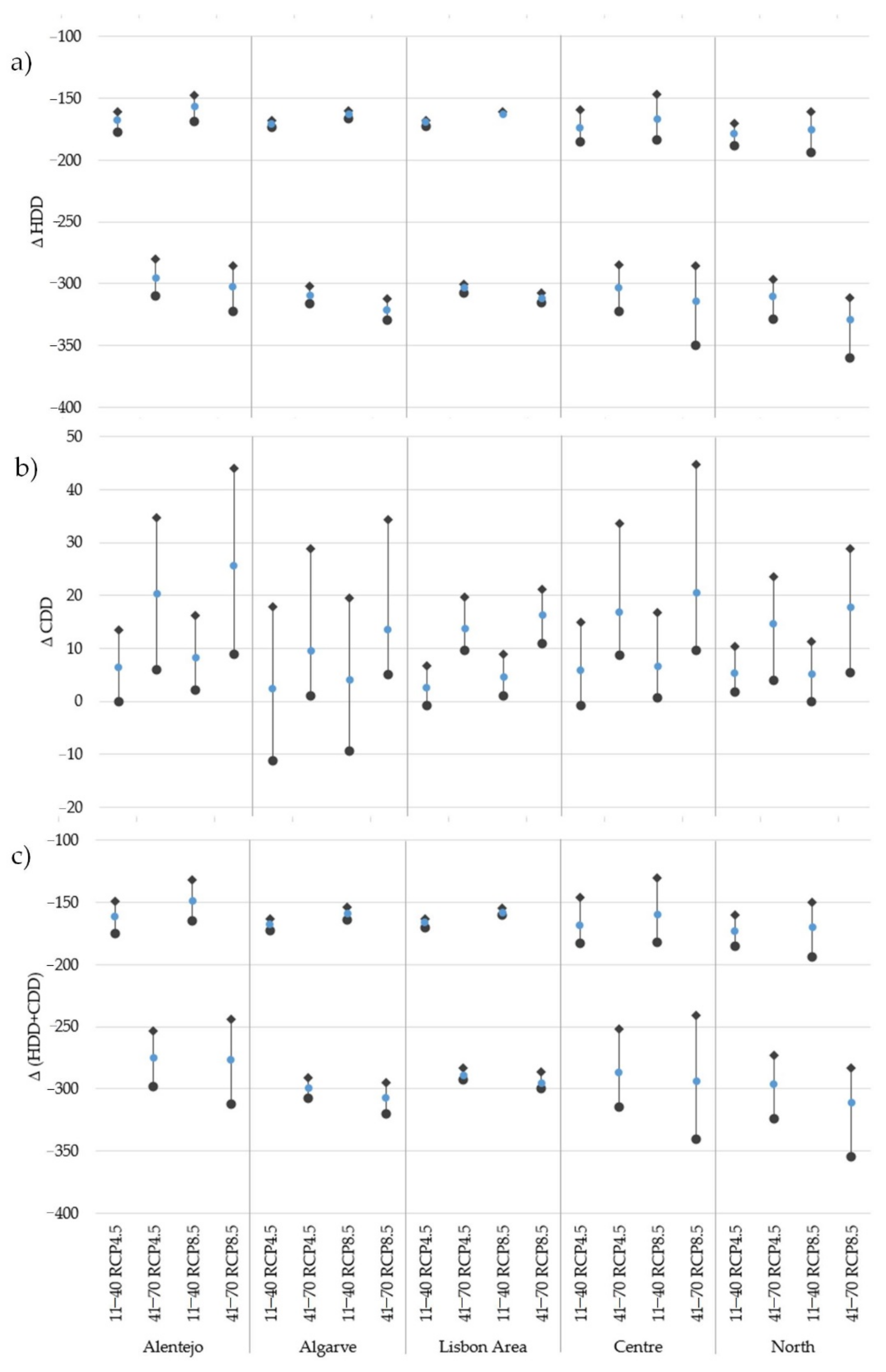
5)

The aggregation of regional changes in HDDs and CDDs to larger areas can be done using area weighting or population weighting (with a fixed population). Population weighting is desirable for assessing energy demand trends over large regions with uneven population distribution, such as Europe. However, due to the size of the study area, this methodology was not followed for Portugal. The case study analysis within the NUTS II region showed that regions with higher projected cooling or heating energy demands present higher increases under both RCPs until 2070. Overall, higher amplitudes were depicted for CDD anomalies in comparison with HDD and HDD + CDD anomalies. Lower HDD and HDD + CDD percentages were found for Algarve and Lisbon Area (LVT in Figure 1), hinting at maritime conditions’ influence to attenuate maximum and minimum temperature contrasts in the future. These amplitudes are predicted to be substantially higher for all indicators for 2041–2070, in which minor differences are projected for HDD and HDD + CDD (Figure 11a,c) and higher for CDD (Figure 11b) under RCP8.5. Results predict that all regions will present fewer heating energy demands for 2011–2040 when comparing with 2041–2070 under RCP8.5 (with higher negative anomalies). Conversely, for all regions, projections point out to lower energy demand for residential heating for both periods under RCP8.5.

All CDD anomalies are positive, foreseeing higher energy demand for cooling, mainly in the inner regions in the south. The increase of energy demand for both periods is evident but higher under RCP8.5, although, for 2041–2070, this rise might reach 45 °C × D per year in certain locations within Alentejo and Center regions (Figure 11b and Table 5).

6)

For each location within the five NUTS II regions a comparison between the historical period 1971–2000 and 2011–2040 and 2041–2070 (under both RCPs) was undertaken. HDD results revealed higher negative percentages for 2041–2070 in comparison with 2011–2040; higher under RCP8.5 (Table 5). Within the five regions for 2041–2070 projections present major values in Algarve and LVT regions, with Faro, Lisboa, and Setúbal with the highest percentages, thus pointing out to a decrease in heating energy demand in these cities. Conversely, HDD anomalies projections reveal that for Bragança in North and Guarda in the Center major heating requirements under both RCPs by 2041–2070 (higher under RCP8.5) will be needed. These results that are quite similar for the ones attained for HDD + CDD anomaly percentages hint at the continentality and latitude as key factors for the heating energy demand, as expected. Still for this indicator, the Center and North regions are projected to present the lowest percentages within the five regions for 2041–2070 under RCP8.5. Like previously, for Bragança in North and Guarda in Center, the lowest percentages for HDD + CDD are projected. Lastly, regarding CDD, results predict positive anomalies, with higher percentages for 2041–2070 under RCP8.5. Highest percentages are projected to be located in the North and Center regions; namely, with predicted percentages above 30% in Bragança (under both RCPs), Viana do Castelo (under RCP8.5), Braga (under RCP8.5), Vila Real (under both RCPs, reaching 41.4% under RCP8.5), Porto (under RCP8.5), and Guarda (under RCP8.5) allow foreseeing an increase of cooling requirements for these cities. Conversely, results for 2041–2070 predict the lower CDD anomaly values to be in Algarve in the southernmost region of Portugal, with 5.3% (the lowest percentage) and 10.1%, under RCP4.5 and RCP8.5, respectively, predicted for the city of Faro.

The Portuguese Regulation on the Energy Performance of Residential Buildings [20], as aforementioned, is in line with the European Directive [22], which aims at reducing the greenhouse gas emissions by 20% by 2020 and in 80% until 2050, in relation to the 1990 emissions levels. This study allowed to conclude that major differences in heating and cooling energy demand can be expected for mainland Portugal under both RCPs and until 2070. The predicted regional differences in residential buildings stock heating and cooling requirements point out the relevance of improving energy efficiency and refurbishment strategies implementing updated sustainable building energetic constraints. To ensure thermal comfort, reduce energy consumption, and reduce greenhouse gas emissions, new policies are needed. Indeed, better construction techniques, the use of new materials, improving thermal quality requirements for new and existing buildings, energy end-uses aspects, as periodic inspection of boilers and air conditioning central systems and integration of renewables energies, as well as energy certification for buildings will be highly relevant towards building a more sustainable future.

References

1. Andrade, C.; Contente, J. Climate change projections for the Worldwide Bioclimatic Classification System in the Iberian Peninsula until 2070. Int. J. Climatol. 2020, 40, 5863–5886. [Google Scholar] [CrossRef]
2. Climate Change 2014: Synthesis Report. Contribution of Working Groups I, II and III to the Fifth Assessment Report of the Intergovernmental Panel on Climate Change; Pachauri, R.K.; Meyer, L.A. (Eds.) IPCC: Geneva, Switzerland, 2014; p. 151. [Google Scholar]
3. Hoegh-Guldberg, O.; Jacob, D.; Bindi, M.; Brown, S.; Camilloni, I.; Diedhiou, A.; Djalante, R.; Ebi, K.; Engelbrecht, F.; Giout, J.; et al. Impacts of 1.5 °C global warming on natural and human systems. In Global Warming of 1.5 °C. An IPCC Special Report on the Impacts of Global Warming of 1.5 °C Above Pre-Industrial Levels and Related Global Greenhouse Gas Emission Pathways, in the Context of Strengthening the Global Response to the Threat of Climate Change, Sustainable Development, and Efforts to Eradicate Poverty; Masson-Delmotte, V., Zhai, P., Pörtner, H.O., Roberts, D., Skea, J., Shukla, P.R., Pirani, A., Moufouma-Okia, W., Péan, C., Pidcock, R., et al., Eds.; IPCC: Geneva, Switzerland, 2018. [Google Scholar]
4. Santos, M.; Fonseca, A.; Fragoso, M.; Santos, J.A. Recent and future changes of precipitation extremes in mainland Portugal. Theor. Appl. Climatol. 2019, 137, 1305–1319. [Google Scholar] [CrossRef]
5. Viceto, C.; Pereira, S.C.; Rocha, A. Climate Change Projections of Extreme Temperatures for the Iberian Peninsula. Atmosphere 2019, 10, 229. [Google Scholar] [CrossRef] [Green Version]
6. Andrade, C.; Rodrigues, S.; Corte-Real, J.A. Preliminary assessment of flood hazard in Nabão River basin using an analytical hierarchy process. AIP Conf. Proc. 2018, 1978. [Google Scholar] [CrossRef]
7. Diffenbaugh, N.S.; Giorgi, F. Climate change hotspots in the CMIP5 global climate model ensemble. Clim. Chang. 2012, 114, 813–822. [Google Scholar] [CrossRef] [PubMed] [Green Version]
8. Andrade, C.; Fraga, H.; Santos, J.A. Climate change multi-model projections for temperature extremes in Portugal. Atmos. Sci. Lett. 2014, 15, 149–156. [Google Scholar] [CrossRef]
9. Andargie, M.S.; Touchie, M.; O’Brien, W. A review of factors affecting occupant comfort in multi-unit residential buildings. Build. Environ. 2019, 160, 106182. [Google Scholar] [CrossRef]
10. Fonseca, A.; Santos, J.A. High resolution temperature datasets in Portugal from a geostatistical approach: Variability and extremes. J. Appl. Meteor. 2018, 57, 627–644. [Google Scholar] [CrossRef]
11. Spinoni, J.; Vogt, J.V.; Barbosa, P.; Dosio, A.; McCormick, N.; Bigano, A.; Füssel, H.-M. Changes of heating and cooling degree-days in Europe from 1981 to 2100. Int. J. Climatol. 2018, 38, e191–e208. [Google Scholar] [CrossRef]
12. Yuan, S.; Stainsby, W.; Li, M.; Xu, K.; Waite, M.; Zimmerle, D.; Feiock, R.; Ramaswami, A.; Modi, V. Future energy scenarios with distributed technology options for residential city blocks in three climate regions of the United States. Appl. Energy 2019, 237, 60–69. [Google Scholar] [CrossRef]
13. van Hooff, T.; Blocken, B.; Hensen, J.L.M.; Timmermans, H.J.P. On the predicted effectiveness of climate adaptation measures for residential buildings. Build. Environ. 2015, 83, 142–158. [Google Scholar] [CrossRef] [Green Version]
14. Semmler, T.; McGrath, R.; Steele-Dunne, S.; Hanafin, J.; Nolan, P.; Wang, S. Influence of climate change on heating and cooling demand in Ireland. Int. J. Climatol. 2010, 30, 1502–1511. [Google Scholar] [CrossRef]
15. Lee, K.; Baek, H.; Cho, C. The estimation of base temperature for heating and cooling degree-days for South Korea. J. Appl. Meteor. 2013, 53, 300–309. [Google Scholar] [CrossRef]
16. Petri, Y.; Caldeira, K. Impacts of global warming on residential heating and cooling degree-days in the United States. Sci. Rep. 2015, 5, 12427. [Google Scholar] [CrossRef] [PubMed] [Green Version]
17. Wang, H.; Chen, Q. Impacts of climate change heating and cooling energy use in buildings in the United States. Energ. Build. 2014, 82, 428–436. [Google Scholar] [CrossRef] [Green Version]
18. Benestad, R.E. Heating Degree Day, Cooling Degree Days, and Precipitation in Europe. Norwegian Meteorological Institute. 2008. Available online: http://met.no/Forskning/Publikasjoner/metno_report/2008/filestore/metno_04-2008.pdf (accessed on 30 October 2020).
19. Aebischer, B.; Catenazzi, G.; Jakob, M. Impact of Climate Change on Thermal Comfort, Heating and Cooling Energy Demand in Europe. ECEE 2007 Summer Study. 2007. Available online: http://www.cepe.ethz.ch/publications/Aebischer_5_110.pdf (accessed on 7 October 2020).
20. Regulation for Energy Performance of Residential Buildings (REPRS in Portuguese). Presidency of the Council of Ministers, Decree-Law 118/2013—Order No 15793-I/2013. Available online: https://dre.pt/pesquisa/-/search/499237/details/maximized (accessed on 1 October 2020).
21. Aguiar, R.; Goncalves, H. Climatologia e Anos Meteorológicos de Referência para o Sistema Nacional de Certificação de Edifícios (Versão 2013); Relatório para ADENE—Agência de Energia; Laboratório Nacional de Energia e Geologia, I.P.: Lisabon, Portugal, 2013; 55p. [Google Scholar]
22. CEC. Energy performance of building directive, Directive 2010/31/EU. Off. J. Eur. Communities 2010, 3, 13–35. [Google Scholar]
23. Goovaerts, P. Geostatistics for Natural Resources Evaluation; Oxford University Press: New York, NY, USA, 1997. [Google Scholar]
24. Hartkamp, A.D.; de Beurs, K.; Stein, A.; White, J.W. Interpolation Techniques for Climate Variables; CIMMYT: Texcoco, Mexico, 1999. [Google Scholar]
25. Goovaerts, P. Geostatistical approaches for incorporating elevation into the spatial interpolation of rainfall. J. Hydrol. 2000, 228, 113–129. [Google Scholar] [CrossRef]
26. Brown, D.P.; Comrie, A.C. Spatial modelling of winter temperature and precipitation in Arizona and New Mexico, USA. Clim. Res. 2002, 22, 115–128. [Google Scholar] [CrossRef]
27. Lloyd, C.D. Assessing the effect of integrating elevation data into the estimation of monthly precipitation in Great Britain. J. Hydrol. 2005, 308, 128–150. [Google Scholar] [CrossRef]
28. Bilgili, B.C.; Erşahin, S.; Özyavuz, M. Spatial Prediction of air temperature in east central Anatolia of Turkey. ISPRS Ann. Photogramm. Remote Sens. Spatial Inf. Sci. 2017, IV-4/W4, 153–159. [Google Scholar] [CrossRef] [Green Version]
29. Available online: https://www.aml.pt/ (accessed on 4 February 2021).
30. Available online: http://portal.amp.pt/ (accessed on 4 February 2021).
31. Andrade, C.; Contente, J. Köppen’s climate classification projections for the Iberian Peninsula. Clim. Res. 2020, 81, 71–89. [Google Scholar] [CrossRef]
32. Cornes, R.; van der Schrier, G.; van den Besselaar, E.J.M.; Jones, P.D. An Ensemble Version of the E-OBS Temperature and Precipitation Datasets. J. Geophys. Res. Atmos. 2018, 123. [Google Scholar] [CrossRef] [Green Version]
33. Taylor, K.E.; Stouffer, R.J.; Meehl, G.A. An Overview of CMIP5 and the Experiment Design. Bull. Amer. Meteor. Soc. 2012, 93, 485–498. [Google Scholar] [CrossRef] [Green Version]
34. Moss, R.H.; Edmonds, J.A.; Hibbard, K.A.; Manning, M.R.; Rose, S.K.; van Vuuren, D.P.; Carter, T.R.; Wilbanks, T.J. The next generation of scenarios for climate change research and assessment. Nature 2010, 463, 747–756. [Google Scholar] [CrossRef] [PubMed]
35. van Vuuren, D.P.; Edmonds, J.; Kainuma, M.; Riahi, K.; Thomson, A.; Hibbard, K.; Hurtt, G.C.; Rose, S.K. The representative concentration pathways: An overview. Clim. Chang. 2011, 109, 5–31. [Google Scholar] [CrossRef]
36. Riahi, K.; Grübler, A.; Nakicenovic, N. Scenarios of long-term socio-economic and environmental development under climate stabilization. Technol. Forecast. Soc. 2007, 74, 887–935. [Google Scholar] [CrossRef]
37. Rao, S.; Riahi, K. The role of Non-CO2 greenhouse gases in climate change mitigation: Long-term scenarios for the 21st century. Energy J. 2006, 27, 177–200. [Google Scholar] [CrossRef]
38. Smith, S.; Wigley, T. Multi-gas forcing stabilization with minicam. Energy J. 2006, 27, 373–391. [Google Scholar] [CrossRef]
39. Clarke, L.; Edmonds, J.; Jacoby, H.; Pitcher, H.; Reilly, J.; Richels, R. Scenarios of Greenhouse Gas Emissions and Atmospheric Concentrations; Sub-Report 2.1a of Synthesis and Assessment Product 2.1 by the U.S. Climate Change Program and the Subcommittee on Global Change Research; Department of Energy, Office of Biological & Environmental Research: Washington, DC, USA, 2007.
40. Wise, M.; Calvin, K.; Thomson, A.; Clarke, L.; Bond-Lamberty, B.; Sands, R.; Smith, S.; Edmonds, J. Implications of limiting CO2 concentrations for land use and energy. Science 2009, 324, 1183–1186. [Google Scholar] [CrossRef]
41. Sivak, M. Potential energy demand for cooling in the 50 largest metropolitan areas of the world: Implications for developing countries. Energy Policy 2009, 37, 1382–1384. [Google Scholar] [CrossRef]
42. Sivak, M. Where to live in the United States: Combined energy demand for heating and cooling in the 50 largest metropolitan areas. Cities 2008, 25, 396–398. [Google Scholar] [CrossRef]
43. Goovaerts, P. Ordinary cokriging revisited. Math. Geol. 1998, 30, 21–42. [Google Scholar] [CrossRef] [Green Version]
44. Isaaks, E.H.; Srivastava, R.M. An Introduction to Applied Geostatistics; Oxford University Press: New York, NY, USA, 1992; 561p. [Google Scholar]
45. Agnew, M.D.; Palutikof, J.P. GIS-based construction of baseline climatologies for the Mediterranean using terrain variables. Clim. Res. 2000, 14, 115–127. [Google Scholar] [CrossRef] [Green Version]
46. Perry, M.; Hollis, D. The generation of monthly gridded datasets for a range of climatic variables over the UK. Int. J. Climatol. 2005, 25, 1041–1054. [Google Scholar] [CrossRef]
47. Arguez, A.; O’Brien, J.J.; Smith, S.R. Air temperature impacts over Eastern North America and Europe associated with low-frequency North Atlantic SST variability. Int. J. Climatol. 2009, 29, 1–10. [Google Scholar] [CrossRef]
48. Daly, C.; Neilson, R.P.; Phillips, D.L. A statistical topographic model for mapping climatological precipitation over mountainous terrain. J. Appl. Meteorol. 1994, 33, 140–158. [Google Scholar] [CrossRef] [Green Version]
49. Morakinyo, T.E.; Ren, C.; Shi, Y.; Lau, K.K.; Tong, H.; Choy, C.; Ng, E. Estimates of the impact of extreme heat events on cooling energy demand in Hong Kong. Renew. Energy 2019, 142, 73–84. [Google Scholar] [CrossRef]
50. Mann, H.B.; Whitney, D.R. On a test of whether one of two random variables is stochastically larger than the other. Ann. Math. Stat. 1947, 50–60. [Google Scholar] [CrossRef]
51. Wilcoxon, F. Individual comparisons by ranking methods. Biom. Bull. 1945, 1, 80–83. [Google Scholar] [CrossRef]
52. Lehmann, E.L. Nonparametrics, Statistical Methods Based on Ranks; Holden-Day Inc.: San Francisco, CA, USA, 1975. [Google Scholar]
53. Sneyers, R. On the Statistical Analysis of Series of Observations; Technical Note nº143; World Meteorological Organization (WMO): Geneva, Switzerland, 1990. [Google Scholar]
54. Theil, H. A rank-invariant method of linear and polynomial regression analysis, I, II, III. Nederl. Akad. Wetensch. Proc. 1950, 53, 386–392, 512–525, 1397–1412. [Google Scholar]
55. Sen, P.K. Estimates of the regression coefficient based on Kendall’s tau. J. Am. Stat. Assoc. 1968, 63, 1379–1389. [Google Scholar] [CrossRef]
56. Spinoni, J.; Vogt, J.; Barbosa, P. European degree-day climatologies and trends for the period 1951–2011. Int. J. Climatol. 2015, 35, 25–36. [Google Scholar] [CrossRef] [Green Version]
Figure 1. Portugal and NUTS II (grey area) location in the Iberian Peninsula.
Atmosphere 12 00715 g001
Figure 2. Methodological framework of this study.
Atmosphere 12 00715 g002
Figure 3. Cumulative distribution functions (CDFs) of the observations (obs, control), ensemble-mean simulation with no bias correction (RCM, control) and bias-corrected ensemble-mean (RCM, cor) for the baseline climate (1971–2000): (a) minimum, and (b) maximum daily temperatures (°C).
Atmosphere 12 00715 g003
Figure 4. Trend analysis polynomials for the historical period (1971–2000) for (a) HDD, (b) CDD, and (c) HDD + CDD, in which East–West trend is represented by the green line, the North–South by the blue line and z-axis represents the variable value.
Atmosphere 12 00715 g004
Figure 5. Mean values (in °C × D per year) of (a) HDD, (b) CDD, and (c) HDD + CDD for the historical period (1971–2000) from E-OBS for Portugal (OK interpolation).
Atmosphere 12 00715 g005
Figure 6. Statistically significant (S.S.) anomalies (Δ) in °C × D per year at a 5% significance level for (a,d) HDD, (b,e) CDD, and (c,f) HDD + CDD between 2011–2040 (upper) and 2041–2070 (lower) under RCP4.5. (Note that Δ = future period − 1961–1990).
Atmosphere 12 00715 g006
Figure 7. Statistically significant (S.S.) anomalies (Δ) in °C × D per year at a 5% significance level for (a,d) HDD, (b,e) CDD, and (c,f) HDD + CDD between 2011–2040 (upper) and 2041–2070 (lower) under RCP8.5. (Note that Δ = future period – 1961–1990).
Atmosphere 12 00715 g007
Figure 8. Statistically significant (S.S.) linear trends (at a 95% confidence level) of (ac) HDD per year, (df) CDD per year, and (g,h,i) HDD + CDD per year under RCP4.5 for 2011–2070 (left), 2041–2070 (center) and 1971–2070 (right).
Atmosphere 12 00715 g008
Figure 9. Statistically significant (S.S.) linear trends (at a 95% confidence level) of (ac) HDD per year, (df) CDD per year, and (gi) HDD + CDD per year under RCP8.5 for 2011–2070 (left), 2041–2070 (center) and 1971–2070 (right).
Atmosphere 12 00715 g009
Figure 10. Annual ensemble-mean values of (a) HDD, (b) CDD, and (c) HDD + CDD for Portugal under RCP4.5 between 2041 and 2070 (blue lines) with the respective statistically significant linear trends (linear regression model equation and R2 coefficient) at a 95% confidence level (orange lines).
Atmosphere 12 00715 g010
Figure 11. Mean (blue dot), Maximum (black square) and Minimum (black dot) values for the anomalies by region (NUTS II) for 2011–2040 and 2041–2070 and both emission scenarios. (a) HDD, (b) CDD, and (c) HDD + CDD in °C × D per year.
Atmosphere 12 00715 g011