Article

The Superiority of Data-Driven Techniques for Estimation of Daily Pan Evaporation

1
Department of Soil and Water Conservation Engineering, College of Technology, G.B. Pant University of Agriculture & Technology, Pantnagar 263145, Uttarakhand, India
2
Department of Civil, Environmental and Natural Resources Engineering, Lulea University of Technology, 97187 Lulea, Sweden
3
Department of Petroleum, Koya Technical Institute, Erbil Polytechnic University, Erbil 44001, Kurdistan, Iraq
4
Department of Farm Machinery and Power Engineering, College of Technology, G.B. Pant University of Agriculture & Technology, Pantnagar 263145, Uttarakhand, India
5
College of Agricultural Engineering, Dr. Rajendra Prasad Central Agriculture University, Pusa 848125, Bihar, India
6
Agricultural Engineering Department, Faculty of Agriculture, Mansoura University, Mansoura 35516, Egypt
7
CERIS, Instituto Superior Técnico, Universidade de Lisboa, 1049-001 Lisboa, Portugal
*
Authors to whom correspondence should be addressed.
Atmosphere 2021, 12(6), 701; https://doi.org/10.3390/atmos12060701
Submission received: 13 April 2021 / Revised: 22 May 2021 / Accepted: 26 May 2021 / Published: 30 May 2021

Abstract

:
In the present study, estimating pan evaporation (Epan) was evaluated based on different input parameters: maximum and minimum temperatures, relative humidity, wind speed, and bright sunshine hours. The techniques used for estimating Epan were the artificial neural network (ANN), wavelet-based ANN (WANN), radial function-based support vector machine (SVM-RF), linear function-based SVM (SVM-LF), and multi-linear regression (MLR) models. The proposed models were trained and tested in three different scenarios (Scenario 1, Scenario 2, and Scenario 3) utilizing different percentages of data points. Scenario 1 includes 60%: 40%, Scenario 2 includes 70%: 30%, and Scenario 3 includes 80%: 20% accounting for the training and testing dataset, respectively. The various statistical tools such as Pearson’s correlation coefficient (PCC), root mean square error (RMSE), Nash–Sutcliffe efficiency (NSE), and Willmott Index (WI) were used to evaluate the performance of the models. The graphical representation, such as a line diagram, scatter plot, and the Taylor diagram, were also used to evaluate the proposed model’s performance. The model results showed that the SVM-RF model’s performance is superior to other proposed models in all three scenarios. The most accurate values of PCC, RMSE, NSE, and WI were found to be 0.607, 1.349, 0.183, and 0.749, respectively, for the SVM-RF model during Scenario 1 (60%: 40% training: testing) among all scenarios. This showed that with an increase in the sample set for training, the testing data would show a less accurate modeled result. Thus, the evolved models produce comparatively better outcomes and foster decision-making for water managers and planners.

1. Introduction

Estimating pan evaporation (PE) is essential for monitoring, surveying, and managing water resources. In many arid and semi-arid regions, water resources are scarce and seriously endangered by overexploitation. Therefore, the precise estimation of evaporation becomes imperative for the planning, managing, and scheduling irrigation practices. Evaporation happens if there is an occurrence of vapor pressure differential between two surfaces, i.e., water and air. The most general and essential meteorological parameters that influence the rate of evaporation are relative humidity, temperature, solar radiation, the deficit of vapor pressure, and wind speed. Thus, for the estimation of evaporation losses, these parameters should be considered for the precise planning and managing of different water supplies [1,2].
In the global hydrological cycle, the evaporation stage is defined as transforming water from a liquid to a vapor state [3]. In recent decades, evaporation losses have increased significantly, especially in semi-arid and arid regions [4,5]. Many factors, such as water budgeting, irrigation water management, hydrology, agronomy, and water supply management require a reliable evaporation rate estimation. The water budgeting factor has been modeled on estimates and the responses of cropping water to varying weather conditions. The daily evaporation of the pan (Epan) was considered a significant parameter. It was widely used as an index of lake and reservoir evaporation, evapotranspiration, and irrigation [6].
It is usually calculated in one of two ways, either (a) directly with pan evaporimeters or (b) indirectly with analytical and semi-empirical models dependent on climatic variables [7,8]. However, the calculation has proved sensitive to multiple sources of error, including strong wind circulation, pan visibility, and water depth measurement in the pan, for various reasons, including physical activity in and around the pan, water litter, and pan construction material and pan height. It can also be a repetitive, costly, and time-consuming process to estimate monthly pan evaporation (EPm) using direct measurement. As a result, in the hydrological field, the introduction of robust and reliable intelligent models is necessary for precise estimation [9,10,11,12,13,14].
Several researchers have used meteorological variables to forecast Epan values, as reported by [15,16,17,18]. Since evaporation is a non-linear, stochastic, and complex operation, a reliable formula to represent all the physical processes involved is difficult to obtain [19]. In recent years, most researchers have commonly acknowledged the use of artificial intelligence techniques, such as artificial neural networks (ANNs), adaptive neuro-fuzzy inference method (ANFIS), and genetic programming (G.P.) in hydrological parameter estimation [15,20,21,22]. In estimating Epan, Sudheer et al. [23] used an ANN. They found that the ANN worked better than the other traditional approach. For modeling western Turkey’s daily pan evaporation, Keskin et al. [24] used a fuzzy approach. To estimate regular Epan, Keskin and Terzi [25] developed multi-layer perceptron (MLP) models. They found that the ANN model showed significantly better performance than the traditional system. Tan et al. [26] applied the ANN methodology to model hourly and daily open water evaporation rates. In regular Epan modeling, Kisi and Çobaner [27] used three distinct ANN methods, namely, the MLP, radial base neural network (RBNN), and generalized regression neural network (GRNN). They found that the MLP and RBNN performed much better than GRNN. In a hot and dry climate, Piri et al. [28] have applied the ANN model to estimate daily Epan. Evaporation estimation methods discussed by Moghaddamnia et al. [19] were implemented based on ANN and ANFIS. The ANN and ANFIS techniques’ findings were considered superior to those of the analytical formulas. The fuzzy sets and ANFIS were used for regular modeling of Epan by Keskin et al. [29] and found that the ANFIS method could be more efficiently used than fuzzy sets in modeling the evaporation process. Dogan et al. [30] used the approach of ANFIS for the calculation of evaporation of the pan from the Yuvacik Dam reservoir, Turkey. Tabari et al. [31] looked at the potential of ANN and multivariate non-linear regression techniques to model normal pan evaporation. Their findings concluded that the ANN performed better than non-linear regression. Using linear genetic programming techniques, Guven and Kişi [20] modeled regular pan evaporation by gene-expression programming (GEP), multi-layer perceptrons (MLP), radial basis neural networks (RBNN), generalized regression neural networks (GRNN), and Stephens–Stewart (SS) models. Two distinct evapotranspiration models have been used and found that the subtractive clustering (SC) model of ANFIS produces reasonable accuracy with less computational amounts than the ANFIS-GP ANN models [32].
A modern universal learning machine proposed by Vapnik (1995) [33] is the support vector machine (SVM), which is applied to both regression [30,34] and pattern recognition. An SVM uses a kernel mapping device to map the input space data to a high-dimensional feature space where the problem is linearly separable. An SVM’s decision function relates to the number of support vectors (S.V.s) and their weights and the kernel chosen a priori, called the kernel [1,21]. Several kinds of kernels are Gaussian and polynomial kernels that may be used [10]. Moreover, artificial neural networks (ANN), wavelet-based artificial neural networks (WANN), support vector machine (SVM) were applied at different combinations of input variables by [23]. Their results showed that ANN, which contains three variables of air temperatures and solar radiation, produces root mean square error (RMSE) of 0.701, mean absolute error (MAE) of 0.525, correlation coefficient (R) of 0.990, and Nash–Sutcliffe efficiency (NSE) of 0.977 had better performances in comparison with WANN and SVR.
In principle, wavelet decomposition emerges as an efficient approximation instrument [18]; that is to say, a set of bases can approximate the random wavelet functions. To approximate Epan, researchers used ANN, WANN, radial function-based support vector machine (SVM-RF), linear function-based support vector machine (SVM-LF), and multi-linear regression (MLR) models of climatic variables.
There have been many studies on the estimation of Epan based on weather variables using data-driven methods. However, the estimation of Epan based on lag-time weather variables, which can be obtained easily, is not standard. After testing different acceptable combinations as input variables, the same inputs were used in artificial intelligence processes. In the proposed study, the main objective is to (1) model Epan using ANN, WANN, SVM-RF, SVM-LF, and MLR models under different scenarios and (2) to select the best-developed model and scenario in Epan estimation based on statistical metrics. The document’s format is as follows. Section 2 contains the study’s materials and methods: Section 3 gives the statistical indexes and methodological properties. The models’ applicability to evaporation prediction and the results are discussed in Section 4. The conclusion is found in Section 5.

2. Materials and Methods

2.1. Study Area and Data Collection

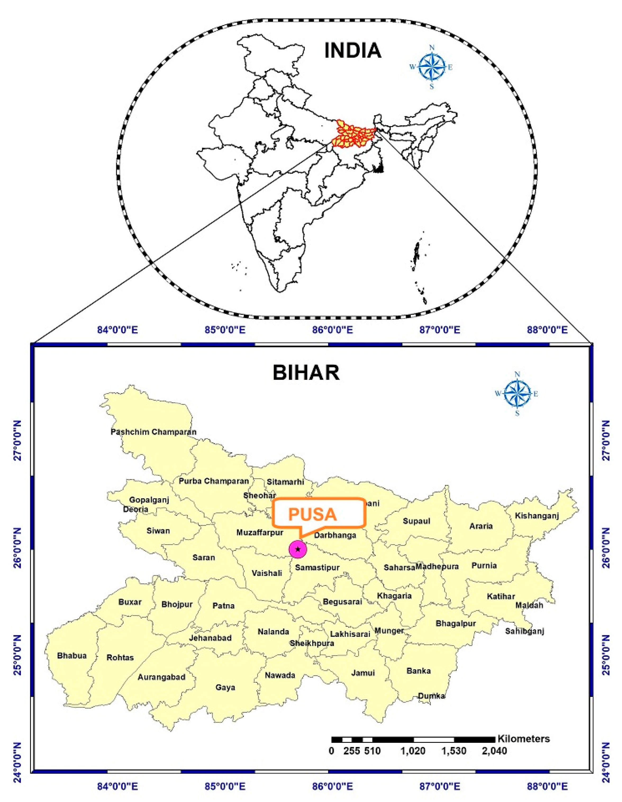
Pusa is located in the Samastipur district of Bihar state, with latitude 25°46′ N and 86°10′ E. The location map of the study area is shown in Figure 1. Pusa lies 53 m above mean sea level in a hot sub-humid agro-ecological region in the middle of the Gangetic plain. The study area is located near the Burhi Ganadak river, a tributary of the Ganges river. The study area is famous for the Dr. Rajendra Prasad Central Agricultural University, a backbone of the study area’s development. The average rainfall for Pusa is 1270 mm, of which 80% of the total rain falls during the monsoon season. The study area is fully covered by the area of the southwest monsoon, which starts in June and eases off in September. The maximum temperature varies from 32 to 38 °C during May and June. The minimum temperature varies from 6 to 9 °C during December and January. The main crops grown in the study area are wheat, maize, paddy, green gram, lentil, potato, and brinjal.
Meteorological data of the study area were gathered from the official “Dr. RPCAU” website (https://www.rpcau.ac.in, accessed on 13 April 2021), Pusa, Bihar. This included maximum and minimum temperatures (Tmax and Tmin, °C), relative humidity (RH-1, percent) at 7 a.m. and at 2 p.m. (RH-2, percent), wind speed (WS, km/h), bright sunshine hours (SSH, h) and daily pan evaporation (EPan, mm). For modeling pan evaporation, five years daily data set between the month 1 June to 30 September means that a total of 610 datasets have been used as input. The same is used for output [35].
Figure 2 displays the climate parameters determined in a box-and-whisker plot between June 2013 and September 2017 (i.e., five-year duration), indicating minimum, first quartile, median, third quartile, and maximum values.
The box-and-whisker plot shows that the relative humidity, measured at 7 am and 2 pm, respectively, demonstrates the highest variability among other meteorological parameters.

2.2. Statistical Analysis

Table 1 presents the statistical analysis of maximum and minimum temperatures (Tmax and Tmin, °C), relative humidity (RH-1, percent) at 7 am and at 2 pm (RH-2, percent), wind speed (WS, km/h), bright sunshine hours (SSH, h) and daily pan evaporation (EPan, mm). The statistical analysis includes mean, median, minimum, maximum, standard deviation (Std. Dev.), kurtosis, and skewness values from 2013 to 2017. The given data is moderate to highly skewed; due to this problem, there has been a considerable negative effect on model performance. The standard deviation for the datasets shows that the values that are farther from zero mean that the variability in the data is higher. Hence, the variation of data from the mean value is higher. The statistical characteristics from the kurtosis values depict the platykurtic and leptokurtic nature of the climatic parameters, where kurtosis values are less than or greater than 3.
Table 2 depicts the inter-correlation between climatic variables at the given station. Thus, it can be observed that all climate parameters have a significant association with the EPan at a significance level of 5%.

2.3. Data-Driven Techniques Used

2.3.1. Artificial Neural Network

The ANN methodology is a tool used to replicate the problem-solving mechanism of the human brain. ANNs are incredibly robust at modeling and simulating linear and non-linear systems. The ANN’s feed-forward back-propagation techniques were highly emphasized among ANNs because their lower level of difficulty in the present study were also used [36,37]. ANN consists of the input layer, output layer, and hidden layers between the input and output layers. Each node within a layer is connected to all the following layer nodes. Only those nodes within one layer are connected to the following layer nodes [29]. Each neuron receives processes and sends the signal to make functional relationships between future and past events. These layers are attached with the interconnected weight Wij and Wjk between the layers of neurons. The typical structure using input variables is shown in Figure 3.
For this analysis, only one hidden layer network was used since it was considered dynamic enough to forecast meteorological variables. There are some transfer functions required to create an artificial neural network neuron. Transfer functions are needed to establish the input–output relationship for each neuron layer. In this analysis, Levenberg–Marquardt was used to train the model. A hyperbolic tangent sigmoid transfer function was used to measure a layer’s output from its net input. The neural network learns by changing the connection weights between the neurons. By using a suitable learning algorithm, the connection weights are altered using the training data set. The number of hidden layers is typically determined by trial and error. A comprehensive ANN overview is available [25,38,39].

2.3.2. Wavelet Artificial Neural Network (WANN)

The wavelet analysis (WA) offers a spectral analysis dependent on the time that explains processes and their relationships in time-frequency space by breaking down time series [40]. WA is an effective method of time-frequency processing, with more benefits than Fourier analysis [41]. WA is an improvement over the Fourier transformation variant used to detect time functionality in data [40]. Wavelet transformation analysis, breaking down time series into essential functions at different frequencies, improves the potential of a predictive model by gathering sufficient information from different resolution levels [25]. There is excellent literature on wavelet transforming theory [42,43]; we will not go into it in depth here. It is vital to choose the base function carefully (called the mother wavelet). The essential functions are generated by translation and dilation [44]. In general, the discrete wavelength transformation (DWT) has been used preferentially in data decomposition, as compared to continuous wavelet transformation (CWT), because CWT is time-consuming [3,18].
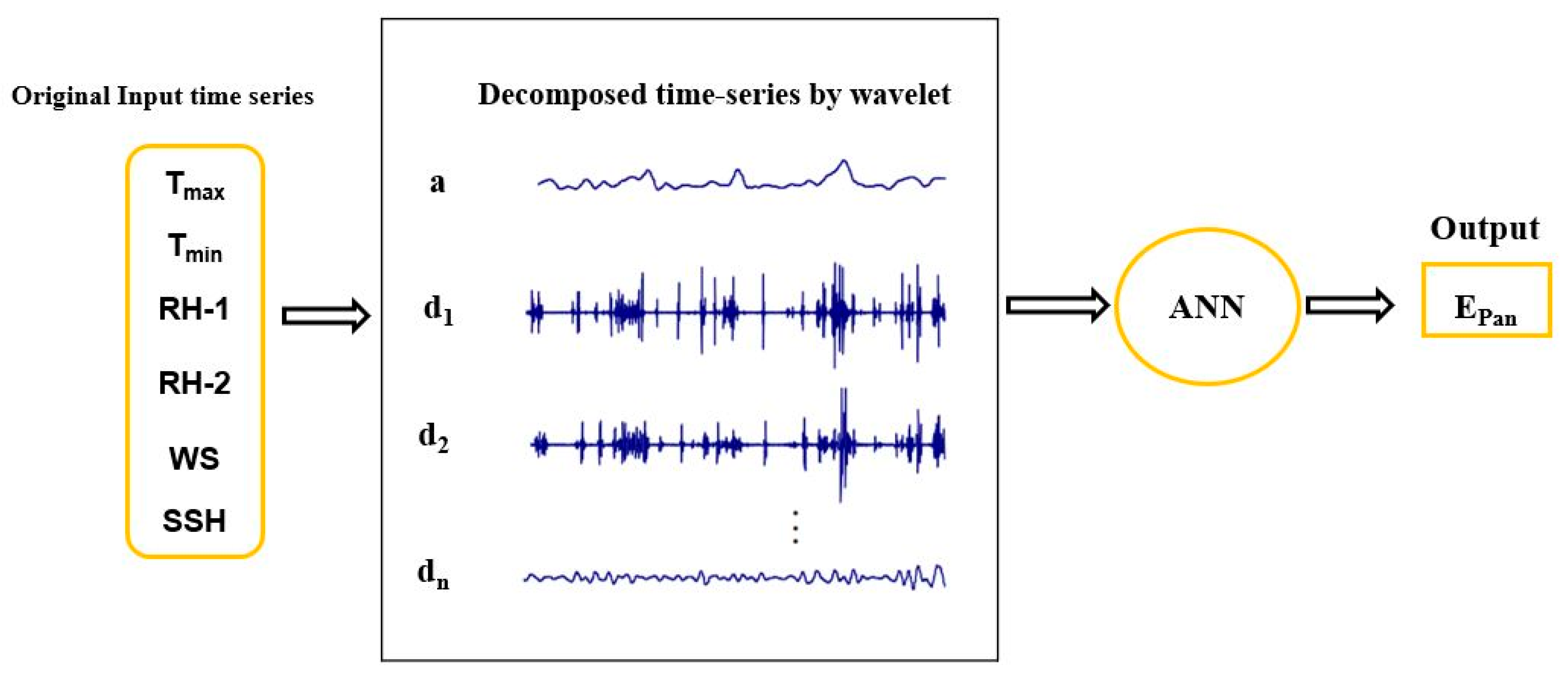
The present used the DWT method for daily EPan (mm) estimation. DWT decomposes the original input time series data of Tmax, Tmin, RH-1, RH-2, WS, and SSH into different frequencies (Figure 4), adapted from Rajaee [44].
This analysis used three stages of the Haar à trous decomposition algorithm using Equations (1) and (2):
C r ( t ) = l = 0 + h ( l ) C r 1 ( t + 2 r )                     ( r = 1 ,   2 ,   3 ,   ,   n )
W r ( t ) = C r 1 ( t ) C r ( t )                                             ( r = 1 ,   2 ,   3 ,   ,   n )
where h ( l ) is the discrete low-pass filter, C r ( t ) and W r ( t ) (r = 1, 2, 3, …., n) are scale coefficient and wavelet coefficient at the resolution level. Two sets of filters, including low and high passes, are employed by DWT to decompose the main time series. It is discontinuous and resembles a step feature that is ideal for certain time series of abrupt transitions. The abovementioned wave types were evaluated, and finally, the measured monthly time series, H, were decomposed into multi-frequency time series including details (HD1; HD2; … ; HDn) and approximation (Ha) by optimum DWT (Qasem et al., 2019).
The obtained decomposed frequency values function as an ANN input. Hybridizing the decomposed input time series data of Tmax, Tmin, RH-1, RH-2, WS, and SSH with ANN results in a wavelet artificial neural network (WANN) [42]. Three levels of the Haar à trous decomposition algorithm were used in this study. For the model’s training, the Levenberg–Marquardt algorithm was used. The hyperbolic tangent sigmoid transfer function was also used to measure a layer’s output from its net input.

2.3.3. Support Vector Machine

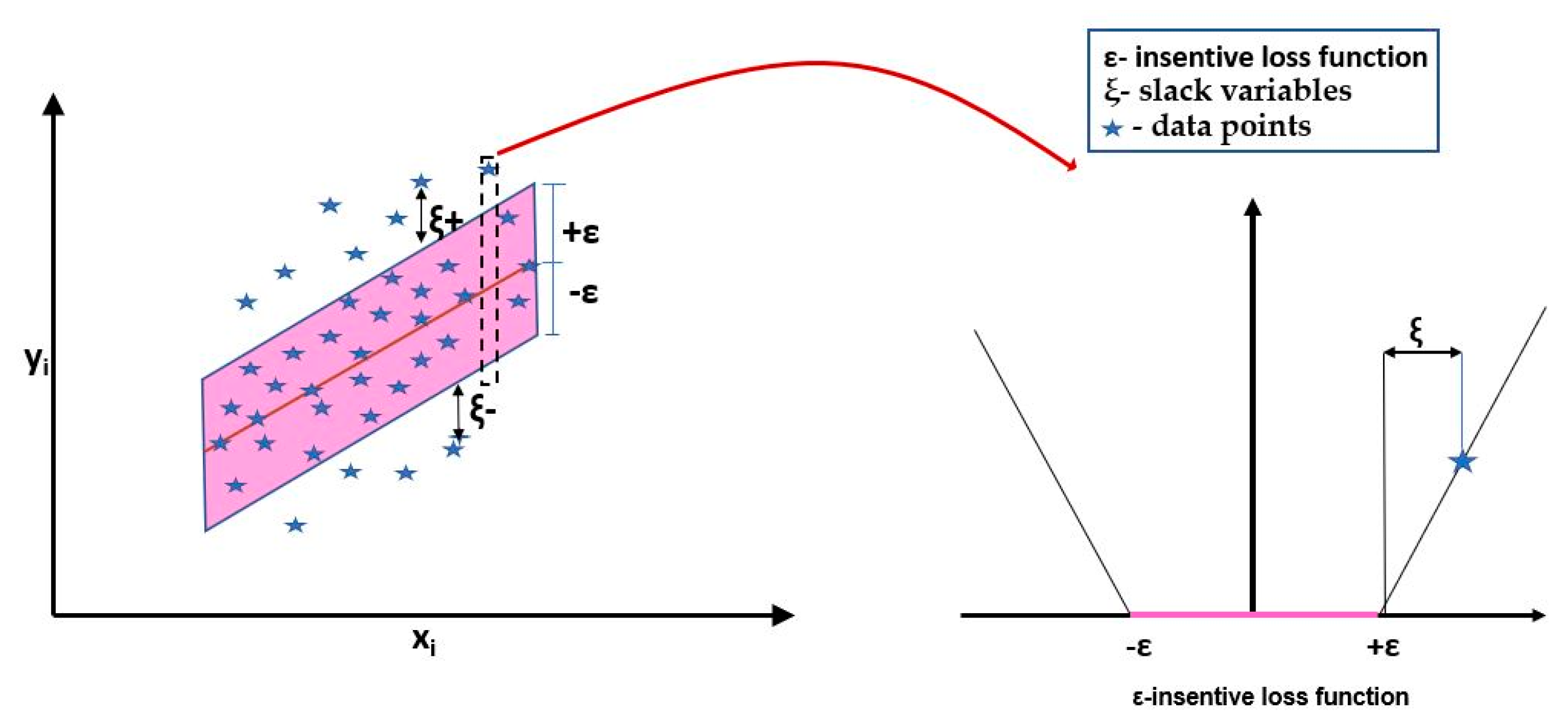
The support vector machine (SVM) was developed by [33] for classification and regression procedures. The fundamental concept of an SVM is to add a kernel function, map the input data by non-linear mapping into a high-dimensional function space, and then perform a linear regression in the feature space [45]. SVM is a modern classifier focused on two principles (Figure 5) adapted from Lin et al. [46]. First, data transformation into a high-dimensional space can render complicated problems easier, utilizing linear discriminate functions. Secondly, SVM is inspired by the training principle and uses only specific inputs nearest to the decision region since they have the most detail regarding classification [47].
We assume a non-linear function f(x) is given by:
f(x) = wTΦ(xi) + b
where w is the weight vector, b is the bias, and Φ(xi) is the high dimensional feature space, linearly mapped from the input space x. Equation (3) can be transformed into higher dimensions and gives final expression as:
f ( x ) = i = 1 m ( α i + α i ) K ( x i ,   x j ) + b ;
where, α i + , α i are Lagrangian multipliers which are used to eliminate some primal variables, and the term K ( x i ,   x j ) is the kernel function. The derivation and excellent literature about SVM can be obtained from [48]. The study’s kernel function was a linear function (LF) and radial function (RF).
  • Linear kernel function (LF): the most basic form of kernel function is written as:
    K ( x i ,   x j ) = ( x i ,   x j )
  • Radial basis function (RBF): a mapping of RBF is identically represented as Gaussian bell shapes:
    K ( x i ,   x j ) = exp ( γ | | x i x j | | 2 )
    where γ is the Gaussian RBF kernel parameter width; the RBF is widely used among all the kernel functions in the SVM technique.
The efficiency of the SVR technique depends on the environment for an ε-insensitive loss function of three training parameters (kernel, C, γ , and ε). However, the values of C and ε influence the complexity of the final model for every specific type of kernel. The ε value measures the number of support vectors (SV) used for predictions. The best value of ε intuitively results in fewer supporting vectors, leading to less complicated regression estimates. However, C’s value is the trade-off between model complexity and the degree of deviations permitted within the optimization formulation. Therefore, a more considerable value of C undermines model complexity [49]. The selection of optimum values for these training parameters (C and ε) guaranteeing fewer complex models is an active research area.

2.3.4. Multiple Linear Regression (MLR)

A linear regression analysis in which more than one independent variable is involved is called MLR. The advantage of MLR is that it is simple, showing how dependent variables interact with independent variables. The overall model of the MLR is:
y = c 0 + c 1 x 1 + c 2 x 2 + + c n x n
where y is the dependent variable, and x1, x2, …, xn are independent variables, c1, c2, …, cn are regression coefficients, and c0 is intercepted. These values are the local behavior calculated using the least square rule or other regression [27].

2.4. Modeling Methodology

In the present study, the daily pan evaporation (EPan) was estimated based on different input climatic variables (Tmax, Tmin, RH-1, RH-2, W.S., and S.S.H.). The five different techniques used for estimation were the artificial neural network (ANN), wavelet-based artificial neural network (WANN), radial function-based support vector machine (SVM-RF), linear function-based support vector machine (SVM-LF), and multi-linear regression (MLR) models. The climatic parameters were collected from 2013 to 2017 and split into three different scenarios, based on the percentage of training and testing datasets for model development (Table 3).
Scenario 1 contains 60% (2013–2015) data for training and 40% (2016–2017) data for testing. Scenario 2 contains 70% data for training and 30% data for testing from 2016. Scenario 3 contains 80% (2013–2016) data for training and 20% (2017) data for testing. The training datasets were used for calibration purposes, while the testing dataset was used for validation purposes.
The results of the applied models in three different scenarios were evaluated through different performance evaluators described in Section 2.5.

2.5. Performance Evaluation Criteria

There were four criteria used to measure the performance of the scenarios mentioned above, quantitatively evaluated using root mean square error (RMSE), Nash–Sutcliffe Efficiency (NSE), Pearson’s correlation coefficient (PCC), and Willmott index (W.I.), and qualitatively evaluated through graphical interpretation (time-series plot, scatter plot, and Taylor diagram). The RMSE range is zero to infinity (0 < RMSE < ∞); the lower the RMSE, the better the model’s performance. The NSE ranges from minus infinity to one (−∞ < NSE < 1). NSE below zero (NSE < 0) indicates that the observed mean only as strong as the average, whereas negative values suggest that the observed mean a more robust indicator than the average [48]. The PCC is also known as the correlation coefficient and is used to calculate the degree of collinearity between observed and estimated values. The PCC varies from minus one to plus one (−1 < PCC < 1) [39]. The WI is also known as the index of agreement. The WI ranges from zero to one (0 < WI < 1); approximately 1 is ideal agreement/fit [3]. The most accurate models were selected based on the highest values of PCC, NSE, and WI, while showing the lowest values of RMSE among all developed models.
R M S E = i = 1 N ( E p o b s , i E p p r e , i ) 2 N ;
N S E = 1 [ i = 1 N ( E p o b s , i E p p r e , i ) 2 i = 1 N ( E p o b s , i E ¯ p o b s , i ) 2 ] ;
PCC   =   i = 1 N ( E p o b s , i E ¯ p o b s , i ) ( E p p r e , i E ¯ p p r e , i ) i = 1 N ( E p o b s , i E ¯ p o b s , i ) 2 i = 1 N ( E p p r e , i E ¯ p p r e , i ) 2 ;
WI = 1 i = 1 N ( E p o b s , i E p p r e , i ) 2 i = 1 N ( | E p p r e , i E ¯ p o b s , i | + | E p o b s , i E ¯ p o b s , i | ) 2 .
where E p o b s , i ,   E p p r e , i observed and predicted pan evaporation values on the ith day. E ¯ p o b s , i ,   E ¯ p p r e , i are average of observed and predicted values, respectively.

3. Results

3.1. Quantitative and Qualitative Evaluation of Results

This section deals with quantitative and qualitative results obtained for the developed models. ANN and WANN trials were conducted depending on the different number of neurons in hidden layers. In contrast, SVM-LF and SVM-RF trials were performed by taking several values of SVM-g, SVM-c, and SVM-e parameters. These were represented in Table 4, Table 5 and Table 6 as a structure for the model.

3.2. Comparison of Training and Testing Datasets for Scenario 1

The training results obtained by ANN, Wavelet, and SVM have been shown in Table 4. As depicted in Table 4, for three developed ANN models, namely ANN-1, ANN-2, and ANN-3, ANN-1 has the highest PCC value of 0.832, the lowest RMSE value of 0.993, the highest NSE value of 0.685, and the highest WI value of 0.904.
Similarly, for the developed WANN model, WANN-1 has shown better performance, with a PCC value of 0.773. Furthermore, the WANN model also has the lowest RMSE value of 1.123, the highest NSE value of 0.597, and the highest WI value of 0.860. Furthermore, among developed SVM-RF and SVM-LF models, SVM-RF-3 has shown better performance than other developed models. The SVM-RF-3 model has the highest PCC value of 0.857; it has the lowest RMSE value of 0.956, the highest NSE value of 0.708, and the highest WI value of 0.895 during training datasets. The value of PCC, RMSE, NSE, and WI for MLR techniques was 0.695, 1.274, 0.483, and 0.800. Thus, it can be stated that SVM-RF has modeled the Epan most efficiently of all the machine learning algorithms developed for training.
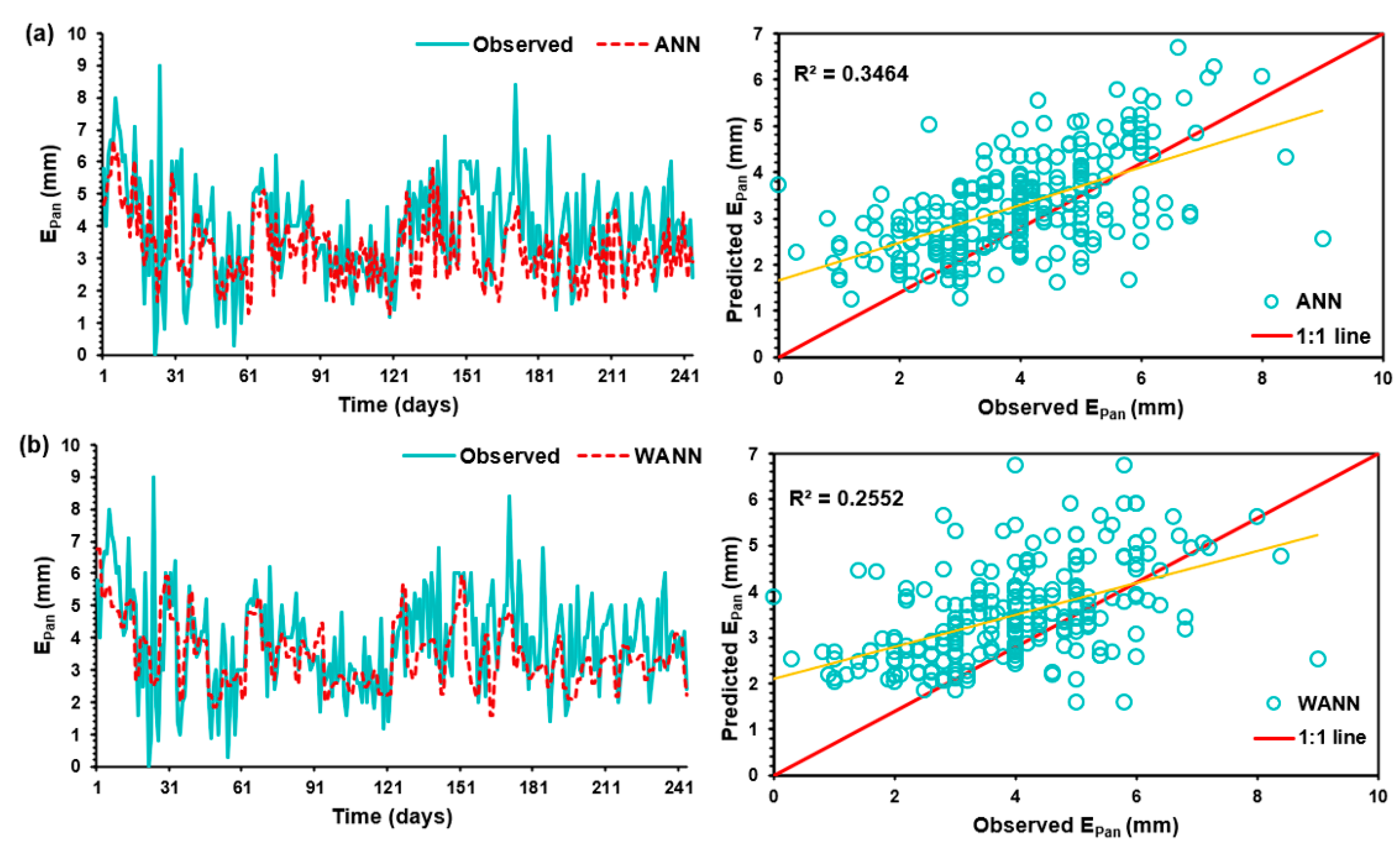
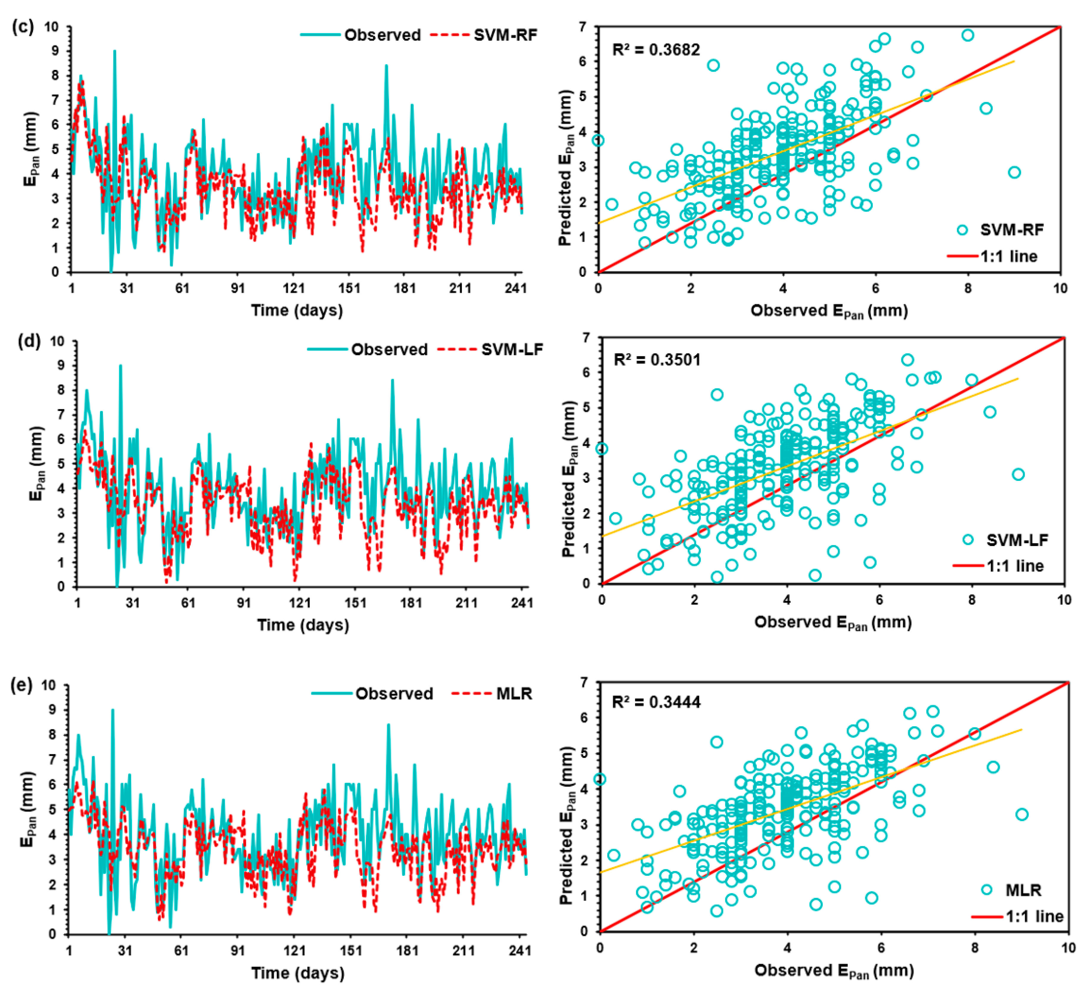
Among developed ANN models, ANN-1 has the highest PCC value of 0.589; it has the lowest RMSE value of 1.387 and the highest NSE value of 0.136. Similarly, for the WANN model, WANN-1 has shown better performance with a PCC value of 0.505, the lowest RMSE value of 1.394, the highest NSE value of 0.129, and a WI value of 0.676.
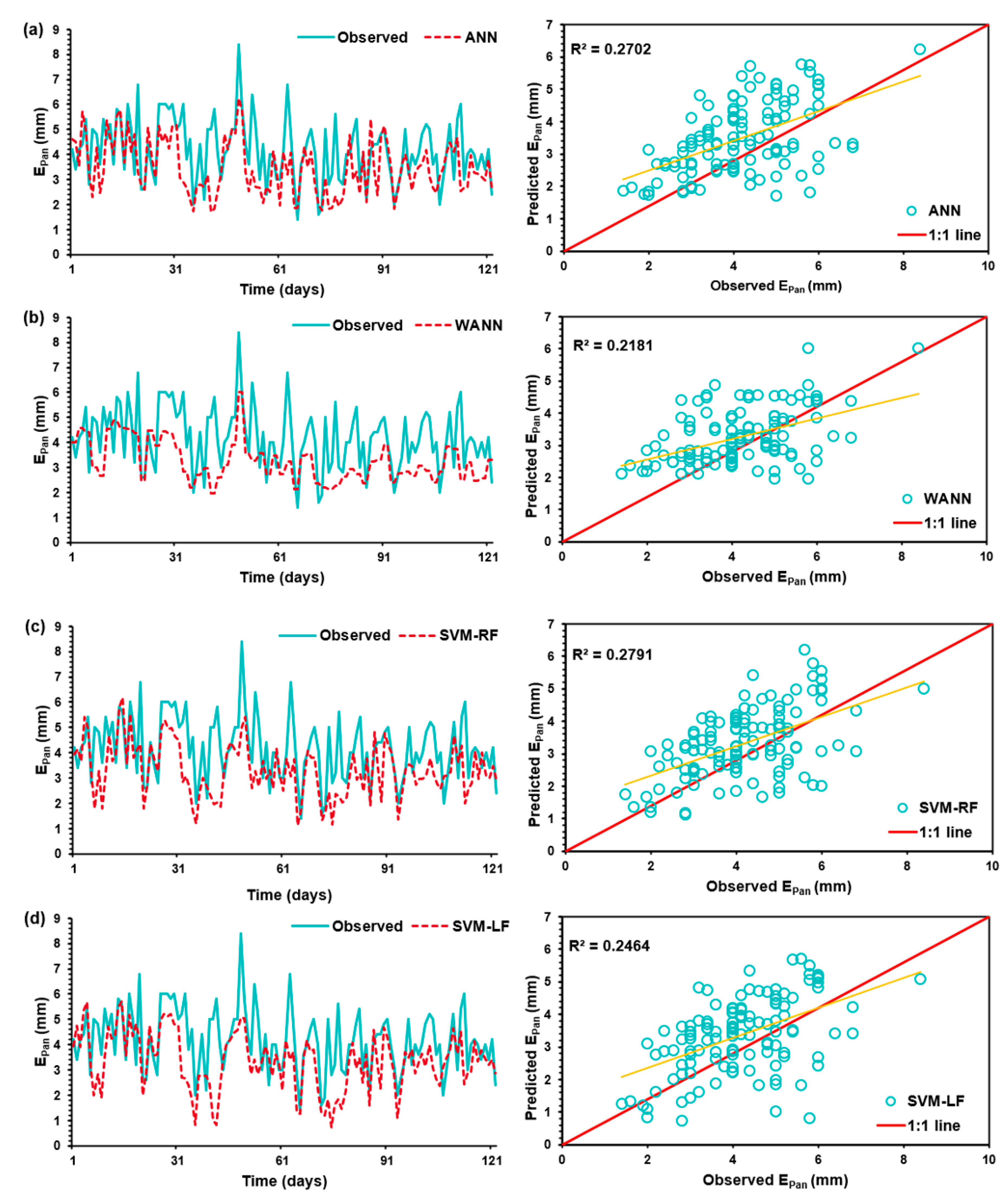
Furthermore, among developed SVM-RF and SVM-LF models, SVM-RF-3 has shown better performance than other developed models. The SVM-RF-3 model has the highest PCC value of 0.607, RMSE value of 1.349, NSE value of 0.183, and the highest WI value of 0.749 training datasets. The values of PCC, RMSE, NSE, and WI for MLR techniques were 0.587, 1.345, 0.188, and 0.725, respectively. The scatter plot and line diagram for the testing data set has been shown in Figure 6. From the line diagram, it can be observed that the obtained results were under-predicted for all models. The scatter plot shows that the highest value of the determination (R2) coefficients was obtained for the SVM-RF model. Thus, it can be suggested that SVM-RF has modeled the Epan most efficiently among all the machine learning algorithms developed for testing.

3.3. Comparison of Training and Testing Datasets for Scenario 2

In Scenario 2, 70% of the entire data set has been used for training, and the rest of the data has been used for testing the developed model. The training results obtained by ANN, Wavelet, and SVM have been shown in Table 5.
As shown in Table 5, among three developed ANN models, the ANN-1 has the highest PCC value of 0.760, the lowest RMSE value of 1.180, the highest NSE value of 0.577, and the highest WI value of 0.854. Similarly, for the WANN model, WANN-2 has shown better performance with a PCC value of 0.725, a lowest RMSE value of 1.264, a highest NSE value of 0.515, and a highest WI value of 0.831. Furthermore, among developed SVM-RF and SVM-LF models, SVM-RF-3 has shown better performance than other developed models. The SVM-RF-3 model has the highest PCC value of 0.812, the lowest RMSE value of 1.262, the highest NSE value of 0.650, and the highest WI value of 0.714 during training datasets. The values of PCC, RMSE, NSE, and WI for MLR techniques were 0.693, 1.308, 0.481, and 0.799, respectively, during training processes. Thus, it can be stated that SVM-RF has modeled the Epan most efficiently among all the machine-learning algorithms developed for training.
For Scenario 2, where 30% of the data set has been used for testing, model ANN-1 has the highest PCC value of 0.547, the lowest RMSE value of 1.222, the highest NSE value of 0.046, and a WI value of 0.704 among ANN models. Similarly, WANN-1 has shown better performance, with a PCC value of 0.457, the lowest RMSE value of 1.252, the highest NSE value of −0.002, and the highest WI value of 0.639 WANN models. Furthermore, SVM-RF-3 has shown better performance as compared to other developed models among SVM-RF and SVM-LF models. The SVM-RF-3 model has the highest PCC value of 0.568, the lowest RMSE value of 1.262, and the highest WI value of 0.714 during training datasets. The values of PCC, RMSE, NSE, and WI for MLR techniques were 0.531, 1.262, −0.017, and 0.700, respectively. The scatter plot and line diagram for testing have been shown in Figure 7. It can be seen from the line diagram that the obtained results were under-predicted for all models. The scatter plot showed that the highest value of the coefficient of determination (R2) was obtained for SVM-RF models of 0.3221. Thus, it can be shown that SVM-RF has modeled the Epan most efficiently among all the machine learning algorithms developed for testing.

3.4. Comparison of Training and Testing Datasets for Scenario 3

In Scenario 3, 80% of the total dataset was used for training periods, while the rest, 20%, was used to test the models. The training results obtained by ANN, wavelet analysis, and SVM have been shown in Table 6.
As depicted from Table 6, for developed ANN models, model ANN-3 has the highest PCC value of 0.520; it has an RMSE value of 1.333 and a W.I. value of 0.688. Similarly, for the WANN model, WANN-1 has shown better performance with a PCC value of 0.725, the lowest RMSE value of 1.213, the highest NSE value of 0.519, and the highest WI value of 0.812. Further, SVM-RF-3 has shown better performance compared to other developed models. The SVM-RF-3 model has the highest PCC value of 0.893, the lowest RMSE value of 0.858, the highest NSE value of 0.760, and the highest WI value of 0.913 during training datasets. The values of PCC, RMSE, NSE, and WI for MLR techniques were 0.688, 1.269, 0.474, and 0.795, respectively. Thus, it can be depicted that SVM-RF has modeled the Epan most efficiently among all the machine learning algorithms developed for training.
For testing datasets, for developed ANN models, ANN-3 has the highest PCC value of 0.520, an RMSE value of 1.333, and the highest W.I. value of 0.688. Similarly, for the WANN model, WANN-1 has shown better performance with a PCC value of 0.467, an RMSE value of 1.447, and WI value of 0.639. Furthermore, among developed SVM-RF and SVM-LF models, SVM-RF-1 has shown better performance than other developed models. The SVM-RF-1 model has the highest PCC value of 0.528, the lowest RMSE value of 1.411, and the highest WI value of 0.665 during the testing of datasets.
The values of PCC, RMSE, NSE, and WI for MLR techniques were 0.506, 1.363, −0.227, and 0.665. The scatter plot and line diagram for testing have been shown in Figure 8. From the line diagram, it has been observed that obtained results were under-predicted and over-predicted for all models. The scatter plot showed that the highest value of the coefficient of determination (R2) was obtained for SVM-RF models of 0.2791. Thus, it can be seen that SVM-RF has modeled the daily Epan most efficiently among all the machine learning algorithms developed for testing.
The comparative results of training and testing data results have been shown in Table 7. This table could suggest that training and testing data using the SVM-RF model, Epan, can be modeled more accurately than ANN and WANN.
The performance of models from best to lowest is SVM > ANN > MLR > WANN for all three scenarios. Table 7 also showed that the WANN model performed poorly compared to other models. This is because wavelet transformation does not reveal the hidden information present in the primary time-series data through different sub-series. It is also observed that, with an increase in the sample set for training, the testing data will show a less accurate modeled result.
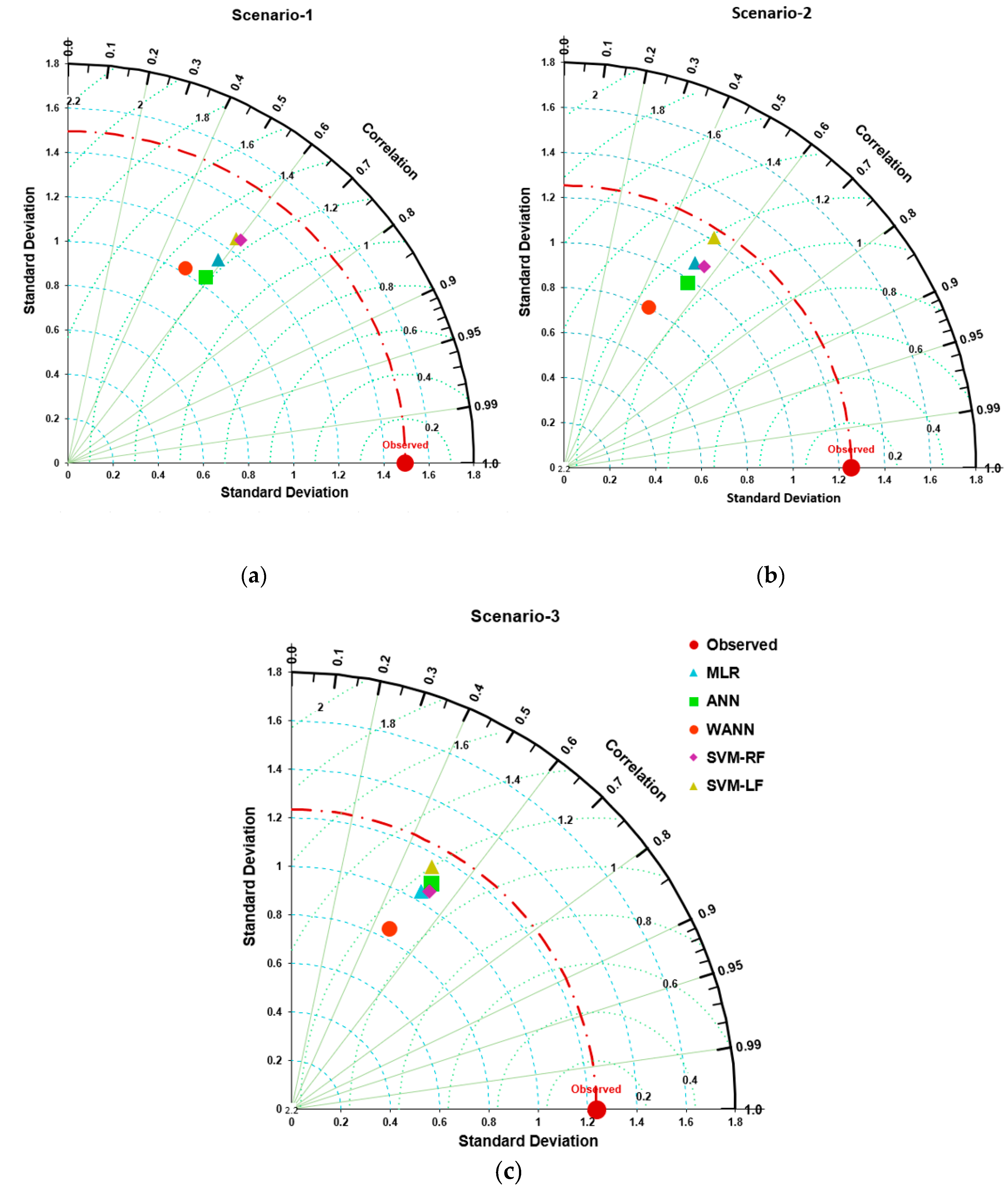
The comparative result of all three scenarios of all developed models has also been shown through Taylor’s diagram [50] in Figure 9a–c, which acquires information based on correlation coefficient, standard deviation, and root mean square difference [27]. Figure 9a–c indicates that the SVM-RF model predictions in all three scenarios are very close to the daily values of Epan, which are tending more toward observed point values at abscissa. The performance-based correlation coefficient, standard deviation, and root mean square difference are also superior compared to others. Therefore, the SVM-RF model with Tmax, Tmin, RH-1, RH-2, WS, and SSH climate variables can be used for daily Epan estimation at the Pusa station.

4. Discussion

Our results as obtained are similar to the results of [17,39]. They modeled pan evaporation and found that the ANN and SVR models achieved high correlation coefficients ranging from 0.81 to 0.90. In addition, our findings are in agreement with Cobaner [15], who observed that the ANN model with Bayesian Regularization (BR) and algorithm during training, validation, and testing generated 0.76, 0.67, and 0.72, respectively. Applying Levenberg–Marquardt (LM) algorithm, the corresponding values were 0.77, 0.69, and 0.71, respectively. Furthermore, for SVR, this model’s findings are close to those of Tezel and Buyukyildiz [51]. They concluded that the SVR gave high correlations, ranging from 0.86 to 0.90, for evaporation forecasting. Moreover, the results obtained with SVR are in line with Pammar and Deka [52]. They stated that the correlation coefficients and RMSE ranged from 0.79 to 0.84 and from 0.90 to 1.03 under the different kernels. The values of RMSE conducted by Alizamir et al. [17] were 0.836 and 0.882 for ANN 4-6-6-1 and 1.028 and 1.106 for MLR models through the training and testing period. Their results found that ANN’s evaporation estimation was better than the estimation through MLR and agreed with the present study results. The ANN model of pan evaporation, with all available variables as inputs, proposed by Rahimi Khoob [21] was the most accurate, delivering an R2 of 0.717 and an RMSE of 1.11 mm independent evaluation data set, which correlates with our outcomes. As reported by Keskin and Terzi [25], the R2 values of the ANN 3, 6, 1, ANN 6, 2, 1, and ANN 7, 2, 1 model equaling 0.770, 0.787, and 0.788 for modeling Epan are also acceptable and agree with our results. These developed models produced a more acceptable outcome than Kim et al. [53]. The latter stated that the ANN and MLR generated R2 values ranging from 0.69 to 0.74 and from 0.61 to 0.64. The RMSE for these models varied from 1.38 to 1.48 and from 1.56 to 1.60, respectively. However, all developed models in this manuscript could not capture the variability of extreme values present in the input and output parameters at the given study location. The models’ efficiency might be improved if the extreme values are removed. This is one of the limitations of the study outlined in this paper.

5. Conclusions

Evaporation processes are strongly non-linear and stochastic phenomena affected by relative humidity, temperature, vapor pressure deficit, and wind speed. In the present study, daily pan evaporation (Epan) estimation was evaluated using ANN, WANN, SVM-RF, SVM-LF, and MLR models. The input climatic variables for the estimation of daily Epan were: maximum and minimum temperatures (Tmax and Tmin), relative humidity (RH-1 and RH-2), wind speed (W.S.), and bright sunshine hours (SSH). The free availability of these meteorological parameters for other stations in Bihar, India, is a significant concern and limitation of this research. The proposed models were trained and tested in three separate scenarios, i.e., Scenario 1, Scenario 2, and Scenario 3, utilizing different percentages of data points. The models above were evaluated using statistical tools, namely, PCC, RMSE, NSE, and WI, through visual inspection using a line diagram, scatter plot, and Taylor diagram. Research results evidenced the SVM-RF model’s ability to estimate daily Epan, integrating all weather details like Tmax, Tmin, RH-1, RH-2, WS, and SSH The SVM-RF model’s dominance was found at Pusa station for all scenarios investigated. It is also clear that, with an increase in the sample set for training, the testing data will show a less accurate modeled result. Since the Pusa dataset has many extreme values, the developed model could not capture extreme values very efficiently; this is one of the limitations of this paper. Overall, the current research outcome showed the SVM-RF model’s viability as a newly established data-intelligent method to simulate pan evaporation in the Indian area. It can be extended to many water resource engineering applications. It is also recommended that SVM-RF models can be applied under the same climatic conditions and the availability of the same meteorological parameters.
Author Contributions

Conceptualization, M.K., A.K. (Anuradha Kumari), D.K. and A.K. (Ambrish Kumar); methodology, M.K. and D.K.; software, M.K., A.K. (Anuradha Kumari) and R.K.; validation, M.K., A.K. (Anuradha Kumari), D.K. and A.K. (Ambrish Kumar); formal analysis, M.K., D.K. and A.K. (Alban Kuriqi); investigation, M.K.; resources, M.K., D.K. and A.K. (Ambrish Kumar); data curation, M.K. and A.K. (Anuradha Kumari); writing—original draft preparation, M.K., A.K. (Anuradha Kumari), R.A. and R.K.; writing—review and editing, M.K., D.K., R.A., A.E. and A.K. (Alban Kuriqi); visualization, D.K., N.A.-A., R.A., A.E. and A.K. (Alban Kuriqi); supervision, D.K., N.A.-A., A.K. (Ambrish Kumar), A.E. and A.K. (Alban Kuriqi); project administration, A.K. (Alban Kuriqi); funding acquisition, N.A-A. Please refer to the CRediT taxonomy for the term explanation. Authorship must be limited to those who have contributed substantially to work reported. All authors have read and agreed to the published version of the manuscript.

Funding

This research received no external funding.

Institutional Review Board Statement

Not applicable.

Informed Consent Statement

Not applicable.

Data Availability Statement

Not available.

Acknowledgments

The authors would like to thank the anonymous reviewers for their valuable comments and suggestions to improve this manuscript further.

Conflicts of Interest

The authors declare no conflict of interest.

References

  1. Alizadeh, M.J.; Kavianpour, M.R.; Kisi, O.; Nourani, V. A new approach for simulating and forecasting the rainfall-runoff process within the next two months. J. Hydrol. 2017, 548, 588–597. [Google Scholar] [CrossRef]
  2. Adnan, R.M.; Liang, Z.; Parmar, K.S.; Soni, K.; Kisi, O. Modeling monthly streamflow in mountainous basin by MARS, GMDH-NN and DENFIS using hydroclimatic data. Neural Comput. Appl. 2021, 33, 2853–2871. [Google Scholar] [CrossRef]
  3. Mbangiwa, N.C.; Savage, M.J.; Mabhaudhi, T. Modelling and measurement of water productivity and total evaporation in a dryland soybean crop. Agric. For. Meteorol. 2019, 266–267, 65–72. [Google Scholar] [CrossRef]
  4. Sayl, K.N.; Muhammad, N.S.; Yaseen, Z.M.; El-shafie, A. Estimation the Physical Variables of Rainwater Harvesting System Using Integrated GIS-Based Remote Sensing Approach. Water Resour. Manag. 2016, 30, 3299–3313. [Google Scholar] [CrossRef]
  5. Sanikhani, H.; Kisi, O.; Maroufpoor, E.; Yaseen, Z.M. Temperature-based modeling of reference evapotranspiration using several artificial intelligence models: Application of different modeling scenarios. Theor. Appl. Climatol. 2019, 135, 449–462. [Google Scholar] [CrossRef]
  6. Rajaee, T.; Nourani, V.; Zounemat-Kermani, M.; Kisi, O. River suspended sediment load prediction: Application of ANN and wavelet conjunction model. J. Hydrol. Eng. 2011, 16, 613–627. [Google Scholar] [CrossRef]
  7. Aytek, A. Co-active neurofuzzy inference system for evapotranspiration modeling. Soft Comput. 2008, 13, 691. [Google Scholar] [CrossRef]
  8. Wang, K.; Liu, X.; Tian, W.; Li, Y.; Liang, K.; Liu, C.; Li, Y.; Yang, X. Pan coefficient sensitivity to environment variables across China. J. Hydrol. 2019, 572, 582–591. [Google Scholar] [CrossRef]
  9. Adnan, R.M.; Liang, Z.; Heddam, S.; Zounemat-Kermani, M.; Kisi, O.; Li, B. Least square support vector machine and multivariate adaptive regression splines for streamflow prediction in mountainous basin using hydro-meteorological data as inputs. J. Hydrol. 2020, 586, 124371. [Google Scholar] [CrossRef]
  10. Snyder, R.L. Equation for Evaporation Pan to Evapotranspiration Conversions. J. Irrig. Drain. Eng. 1992, 118, 977–980. [Google Scholar] [CrossRef]
  11. Adnan, R.M.; Liang, Z.; Trajkovic, S.; Zounemat-Kermani, M.; Li, B.; Kisi, O. Daily streamflow prediction using optimally pruned extreme learning machine. J. Hydrol. 2019, 577, 123981. [Google Scholar] [CrossRef]
  12. Yuan, X.; Chen, C.; Lei, X.; Yuan, Y.; Muhammad Adnan, R. Monthly runoff forecasting based on LSTM–ALO model. Stoch. Environ. Res. Risk Assess. 2018, 32, 2199–2212. [Google Scholar] [CrossRef]
  13. Zerouali, B.; Al-Ansari, N.; Chettih, M.; Mohamed, M.; Abda, Z.; Santos, C.A.G.; Zerouali, B.; Elbeltagi, A. An Enhanced Innovative Triangular Trend Analysis of Rainfall Based on a Spectral Approach. Water 2021, 13, 727. [Google Scholar] [CrossRef]
  14. Malik, A.; Rai, P.; Heddam, S.; Kisi, O.; Sharafati, A.; Salih, S.Q.; Al-Ansari, N.; Yaseen, Z.M. Pan Evaporation Estimation in Uttarakhand and Uttar Pradesh States, India: Validity of an Integrative Data Intelligence Model. Atmosphere 2020, 11, 553. [Google Scholar] [CrossRef]
  15. Cobaner, M. Evapotranspiration estimation by two different neuro-fuzzy inference systems. J. Hydrol. 2011, 398, 292–302. [Google Scholar] [CrossRef]
  16. Muhammad Adnan, R.; Chen, Z.; Yuan, X.; Kisi, O.; El-Shafie, A.; Kuriqi, A.; Ikram, M. Reference Evapotranspiration Modeling Using New Heuristic Methods. Entropy 2020, 22, 547. [Google Scholar] [CrossRef]
  17. Alizamir, M.; Kisi, O.; Muhammad Adnan, R.; Kuriqi, A. Modelling reference evapotranspiration by combining neuro-fuzzy and evolutionary strategies. Acta Geophys. 2020, 68, 1113–1126. [Google Scholar] [CrossRef]
  18. Vallet-Coulomb, C.; Legesse, D.; Gasse, F.; Travi, Y.; Chernet, T. Lake evaporation estimates in tropical Africa (Lake Ziway, Ethiopia). J. Hydrol. 2001, 245, 1–18. [Google Scholar] [CrossRef]
  19. Moghaddamnia, A.; Ghafari Gousheh, M.; Piri, J.; Amin, S.; Han, D. Evaporation estimation using artificial neural networks and adaptive neuro-fuzzy inference system techniques. Adv. Water Resour. 2009, 32, 88–97. [Google Scholar] [CrossRef]
  20. Guven, A.; Kişi, Ö. Daily pan evaporation modeling using linear genetic programming technique. Irrig. Sci. 2011, 29, 135–145. [Google Scholar] [CrossRef]
  21. Rahimi Khoob, A. Artificial neural network estimation of reference evapotranspiration from pan evaporation in a semi-arid environment. Irrig. Sci. 2008, 27, 35–39. [Google Scholar] [CrossRef]
  22. Trajkovic, S. Testing hourly reference evapotranspiration approaches using lysimeter measurements in a semiarid climate. Hydrol. Res. 2009, 41, 38–49. [Google Scholar] [CrossRef]
  23. Sudheer, K.P.; Gosain, A.K.; Mohana Rangan, D.; Saheb, S.M. Modelling evaporation using an artificial neural network algorithm. Hydrol. Process. 2002, 16, 3189–3202. [Google Scholar] [CrossRef]
  24. Keskin, M.E.; Terzi, Ö.; Taylan, D. Fuzzy logic model approaches to daily pan evaporation estimation in western Turkey/Estimation de l’évaporation journalière du bac dans l’Ouest de la Turquie par des modèles à base de logique floue. Hydrol. Sci. J. 2004, 49, 1010. [Google Scholar] [CrossRef]
  25. Keskin, M.E.; Terzi, Ö. Artificial Neural Network Models of Daily Pan Evaporation. J. Hydrol. Eng. 2006, 11, 65–70. [Google Scholar] [CrossRef]
  26. Tan, S.B.K.; Shuy, E.B.; Chua, L.H.C. Modelling hourly and daily open-water evaporation rates in areas with an equatorial climate. Hydrol. Process. Int. J. 2007, 21, 486–499. [Google Scholar] [CrossRef]
  27. Kisi, Ö.; Çobaner, M. Modeling River Stage-Discharge Relationships Using Different Neural Network Computing Techniques. CLEAN Soil Air Water 2009, 37, 160–169. [Google Scholar] [CrossRef]
  28. Piri, J.; Amin, S.; Moghaddamnia, A.; Keshavarz, A.; Han, D.; Remesan, R. Daily Pan Evaporation Modeling in a Hot and Dry Climate. J. Hydrol. Eng. 2009, 14, 803–811. [Google Scholar] [CrossRef]
  29. Keskin, M.E.; Terzi, Ö.; Taylan, D. Estimating daily pan evaporation using adaptive neural-based fuzzy inference system. Theor. Appl. Climatol. 2009, 98, 79–87. [Google Scholar] [CrossRef]
  30. Dogan, E.; Gumrukcuoglu, M.; Sandalci, M.; Opan, M. Modelling of evaporation from the reservoir of Yuvacik dam using adaptive neuro-fuzzy inference systems. Eng. Appl. Artif. Intell. 2010, 23, 961–967. [Google Scholar] [CrossRef]
  31. Tabari, H.; Marofi, S.; Sabziparvar, A.-A. Estimation of daily pan evaporation using artificial neural network and multivariate non-linear regression. Irrig. Sci. 2010, 28, 399–406. [Google Scholar] [CrossRef]
  32. Chu, H.-J.; Chang, L.-C. Application of Optimal Control and Fuzzy Theory for Dynamic Groundwater Remediation Design. Water Resour. Manag. 2009, 23, 647–660. [Google Scholar] [CrossRef]
  33. Vapnik, V. The Nature of Statistical Learning Theory; Springer: New York, NY, USA, 1995. [Google Scholar]
  34. Kim, S.; Shiri, J.; Kisi, O. Pan Evaporation Modeling Using Neural Computing Approach for Different Climatic Zones. Water Resour. Manag. 2012, 26, 3231–3249. [Google Scholar] [CrossRef]
  35. Tikhamarine, Y.; Malik, A.; Pandey, K.; Sammen, S.S.; Souag-Gamane, D.; Heddam, S.; Kisi, O. Monthly evapotranspiration estimation using optimal climatic parameters: Efficacy of hybrid support vector regression integrated with whale optimization algorithm. Environ. Monit. Assess. 2020, 192, 696. [Google Scholar] [CrossRef]
  36. Elbeltagi, A.; Deng, J.; Wang, K.; Hong, Y. Crop Water footprint estimation and modeling using an artificial neural network approach in the Nile Delta, Egypt. Agric. Water Manag. 2020, 235, 106080. [Google Scholar] [CrossRef]
  37. Elbeltagi, A.; Aslam, M.R.; Malik, A.; Mehdinejadiani, B.; Srivastava, A.; Bhatia, A.S.; Deng, J. The impact of climate changes on the water footprint of wheat and maize production in the Nile Delta, Egypt. Sci. Total Environ. 2020, 743, 140770. [Google Scholar] [CrossRef] [PubMed]
  38. Elbeltagi, A.; Deng, J.; Wang, K.; Malik, A.; Maroufpoor, S. Modeling long-term dynamics of crop evapotranspiration using deep learning in a semi-arid environment. Agric. Water Manag. 2020, 241, 106334. [Google Scholar] [CrossRef]
  39. Elbeltagi, A.; Aslam, M.R.; Mokhtar, A.; Deb, P.; Abubakar, G.A.; Kushwaha, N.L.; Venancio, L.P.; Malik, A.; Kumar, N.; Deng, J. Spatial and temporal variability analysis of green and blue evapotranspiration of wheat in the Egyptian Nile Delta from 1997 to 2017. J. Hydrol. 2020, 125662. [Google Scholar] [CrossRef]
  40. Kim, T.-W.; Valdés, J.B. Nonlinear Model for Drought Forecasting Based on a Conjunction of Wavelet Transforms and Neural Networks. J. Hydrol. Eng. 2003, 8, 319–328. [Google Scholar] [CrossRef] [Green Version]
  41. Adamowski, J.; Fung Chan, H.; Prasher, S.O.; Ozga-Zielinski, B.; Sliusarieva, A. Comparison of multiple linear and nonlinear regression, autoregressive integrated moving average, artificial neural network, and wavelet artificial neural network methods for urban water demand forecasting in Montreal, Canada. Water Resour. Res. 2012, 48. [Google Scholar] [CrossRef]
  42. Labat, D.; Ababou, R.; Mangin, A. Rainfall–runoff relations for karstic springs. Part II: Continuous wavelet and discrete orthogonal multiresolution analyses. J. Hydrol. 2000, 238, 149–178. [Google Scholar] [CrossRef]
  43. Kişi, Ö. Daily suspended sediment estimation using neuro-wavelet models. Int. J. Earth Sci. 2010, 99, 1471–1482. [Google Scholar] [CrossRef]
  44. Rajaee, T. Wavelet and ANN combination model for prediction of daily suspended sediment load in rivers. Sci. Total Environ. 2011, 409, 2917–2928. [Google Scholar] [CrossRef]
  45. Adnan, R.M.; Khosravinia, P.; Karimi, B.; Kisi, O. Prediction of hydraulics performance in drain envelopes using Kmeans based multivariate adaptive regression spline. Appl. Soft Comput. 2021, 100, 107008. [Google Scholar] [CrossRef]
  46. Lin, J.-Y.; Cheng, C.-T.; Chau, K.-W. Using support vector machines for long-term discharge prediction. Hydrol. Sci. J. 2006, 51, 599–612. [Google Scholar] [CrossRef]
  47. Tripathi, S.; Srinivas, V.V.; Nanjundiah, R.S. Downscaling of precipitation for climate change scenarios: A support vector machine approach. J. Hydrol. 2006, 330, 621–640. [Google Scholar] [CrossRef]
  48. Liu, Q.-J.; Shi, Z.-H.; Fang, N.-F.; Zhu, H.-D.; Ai, L. Modeling the daily suspended sediment concentration in a hyperconcentrated river on the Loess Plateau, China, using the Wavelet–ANN approach. Geomorphology 2013, 186, 181–190. [Google Scholar] [CrossRef]
  49. Cherkassky, V.; Ma, Y. Practical selection of SVM parameters and noise estimation for SVM regression. Neural Netw. 2004, 17, 113–126. [Google Scholar] [CrossRef] [Green Version]
  50. Taylor, K.E. Summarizing multiple aspects of model performance in a single diagram. J. Geophys. Res. Atmos. 2001, 106, 7183–7192. [Google Scholar] [CrossRef]
  51. Tezel, G.; Buyukyildiz, M. Monthly evaporation forecasting using artificial neural networks and support vector machines. Theor. Appl. Climatol. 2016, 124, 69–80. [Google Scholar] [CrossRef]
  52. Pammar, L.; Deka, P.C. Daily pan evaporation modeling in climatically contrasting zones with hybridization of wavelet transform and support vector machines. Paddy Water Environ. 2017, 15, 711–722. [Google Scholar] [CrossRef]
  53. Kim, S.; Singh, V.P.; Seo, Y. Evaluation of pan evaporation modeling with two different neural networks and weather station data. Theor. Appl. Climatol. 2014, 117, 1–13. [Google Scholar] [CrossRef]
Figure 1. Location map of the study area.
Atmosphere 12 00701 g001
Figure 2. Box-and-whisker plot of climatic parameters in the study area.
Atmosphere 12 00701 g002
Figure 3. Three-layered structure of the artificial neural network.
Atmosphere 12 00701 g003
Figure 4. Schematic representation of WANN.
Atmosphere 12 00701 g004
Figure 5. SVM Layout.
Atmosphere 12 00701 g005
Figure 6. Line and scatter plot between observed and predicted data at Scenario 1 for (a) ANN, (b) WANN (c) SVM-RF, (d) SVM-LF, and (e) MLR for the study area.
Atmosphere 12 00701 g006aAtmosphere 12 00701 g006b
Figure 7. Line and scatter plots between observed and predicted data at Scenario 2 for (a) ANN, (b) WANN (c) SVM-RF, (d) SVM-LF, and (e) MLR, for the study area.
Atmosphere 12 00701 g007
Figure 8. Line and scatter plot between observed and predicted data at scenario 3 for (a) ANN, (b) WANN (c) SVM-RF, (d) SVM-LF, and (e) MLR, for the study area.
Atmosphere 12 00701 g008aAtmosphere 12 00701 g008b
Figure 9. Taylor diagrams of ANN, WANN, SVM-RF, SVM-LF, and MLR corresponding to (a) Scenario 1, (b) Scenario 2, (c) Scenario 3 during the testing period at the study site.
Atmosphere 12 00701 g009
Table 1. Statistical constraints of climatic parameters from 2013 to 2017 in the study area.
Statistical ParametersMeanMedianMinimumMaximumStd. Dev.KurtosisSkewness
Tmax (°C)33.5833.8023.4042.702.431.30−0.11
Tmin (°C)25.8726.0021.4029.601.310.37−0.51
RH-1 (%)88.4289.0055.0098.005.394.27−1.33
RH-2 (%)68.8368.0023.0097.0012.170.65−0.22
WS (km/h)6.035.701.2016.702.630.820.85
SSH (h)5.365.550.0012.703.50−1.20−0.02
EPan (mm)3.853.700.0013.001.672.340.89
Table 2. Intercorrelation values between climatic parameters in the study area.
Climatic VariableTmaxTminRH-1RH-2WSSSHEPan
Tmax1.00
Tmin0.321.00
RH-1−0.43−0.291.00
RH-2−0.51−0.150.481.00
WS−0.070.02−0.190.001.00
SSH0.680.28−0.42−0.510.051.00
EPan0.580.11−0.30−0.340.190.511.00
Table 3. Different scenarios of training and testing datasets used in this study.
ScenariosTraining Data Length (%)Testing Data Length (%)
Scenario 160% (2013–2015)40% (2016–2017)
Scenario 270%30%
Scenario 380% (2013–2016)20% (2017)
Table 4. Results for ANN, WANN, SVM-RF, SVM-LF, and M.L.R. during the training and testing period for Scenario 1 (60–40: Training–Testing).
ModelStructureDatasetPCCRMSENSEWI
ANN-16-5-1Training0.8320.9930.6850.904
Testing0.5891.3870.1360.708
ANN-26-8-1Training0.7391.2540.4980.840
Testing0.5851.4860.0100.732
ANN-36-12-1Training0.7691.1570.5730.846
Testing0.5311.529−0.0480.705
WANN-124-6-1Training0.7731.1230.5970.860
Testing0.5051.3940.1290.676
WANN-224-11-1Training0.6941.2860.4720.813
Testing0.4281.4910.0030.614
WANN-324-16-1Training0.6341.5020.2810.766
Testing0.4771.643−0.2110.681
SVM-RF-1c = 1, ε = 0.001, γ = 0.16Training0.7771.1220.5990.856
Testing0.5951.3690.1590.746
SVM-RF-2c = 1, ε = 0.01, γ = 0.16Training0.7941.0880.6220.864
Testing0.6041.3440.1900.749
SVM-RF-3c = 1, ε = 0.1, γ = 0.16Training0.8570.9560.7080.895
Testing0.6071.3490.1830.749
SVM-LF-1c = 1, ε = 0.1, γ = 0.5Training0.6871.2970.4630.804
Testing0.5921.4060.1130.731
SVM-LF-2c = 1, ε = 0.1, γ = 0.8Training0.6871.2970.4630.804
Testing0.5921.4060.1130.731
SVM-LF-3c = 1, ε = 0.1, γ = 0.16Training0.6871.2970.4630.807
Testing0.5921.4060.1130.731
MLR Training0.6951.2740.4830.800
Testing0.5871.3450.1880.725
Table 5. Results for ANN, WANN, SVM-RF, SVM-LF, and MLR during training and testing period for Scenario 2 (70–30: Training–Testing).
ModelStructureDatasetPCCRMSENSEWI
ANN-16-1-1Training0.7601.1800.5770.854
Testing0.5471.2220.0460.704
ANN-26-4-1Training0.7491.2090.5570.842
Testing0.5351.333−0.1350.691
ANN-36-10-1Training0.7161.2780.5040.824
Testing0.5461.2350.0260.727
WANN-124-1-1Training0.6721.3440.4520.781
Testing0.4391.316−0.1060.602
WANN-224-6-1Training0.7251.2640.5150.831
Testing0.4571.252−0.0020.639
WANN-324-9-1Training0.7161.2810.5020.802
Testing0.4131.275−0.0390.604
SVM-RF-1c = 1, ε = 0.001, γ = 0.16Training0.7641.1780.5790.847
Testing0.5601.285−0.0550.704
SVM-RF-2c = 1, ε = 0.01, γ = 0.16Training0.7651.1770.5790.848
Testing0.5611.286−0.0560.705
SVM-RF-3c = 1, ε = 0.1, γ = 0.16Training0.8121.0730.6500.875
Testing0.5681.262−0.0180.714
SVM-LF-1c = 1, ε = 0.1, γ = 0.9Training0.6891.3260.4660.805
Testing0.5391.356−0.1750.696
SVM-LF-2c = 1, ε = 0.01, γ = 0.16Training0.6881.3300.4630.807
Testing0.5421.360−0.1820.700
SVM-LF-3c = 1, ε = 0.1, γ = 0.16Training0.6891.3260.4660.805
Testing0.5391.356−0.1750.696
MLR Training0.6931.3080.4810.799
Testing0.5311.262−0.0170.700
Table 6. Results for ANN, WANN, SVM-RF, SVM-LF, and M.L.R. during the training and testing period for Scenario 3 (80–20: Training–Testing).
ModelStructureDatasetPCCRMSENSEWI
ANN-16-1-1Training0.7011.2500.4900.809
Testing0.5121.321−0.1520.681
ANN-26-9-1Training0.7641.1360.5780.847
Testing0.5141.260−0.0490.695
ANN-36-13-1Training0.7891.0790.6200.879
Testing0.5201.333−0.1720.688
WANN-124-2-1Training0.7251.2130.5190.812
Testing0.4671.447−0.3820.608
WANN-224-7-1Training0.6931.2670.4760.813
Testing0.3691.434−0.3570.586
WANN-324-11-1Training0.7211.2210.5130.812
Testing0.4391.334−0.1750.603
SVM-RF-1c = 1, ε = 0.001, γ = 0.16Training0.7681.1280.5840.849
Testing0.5271.415−0.3220.660
SVM-RF-2c = 1, ε = 0.1, γ = 0.2Training0.8500.9510.7050.894
Testing0.5261.413−0.3180.664
SVM-RF-3c = 1, ε = 0.1, γ = 0.16Training0.8930.8580.7600.913
Testing0.5281.411−0.3150.665
SVM-LF-1c = 1, ε = 0.1, γ = 0.3Training0.6841.2860.4600.802
Testing0.4961.453−0.3940.658
SVM-LF-2c = 1, ε = 0.1, γ = 0.6Training0.6841.2860.4600.802
Testing0.4961.453−0.3940.658
SVM-LF-3c = 1, ε = 0.001, γ = 0.16Training0.6831.2860.4600.803
Testing0.4901.465−0.4170.654
MLR Training0.6881.2690.4740.795
Testing0.5061.363−0.2270.665
Table 7. Results for best ANN, WANN, SVM-RF, and MLR during the training and testing period for all scenarios.
ScenarioModelDatasetPCCRMSENSEWI
1ANN-1Training0.8320.9930.6850.904
Testing0.5891.3870.1360.708
WANN-1Training0.7731.1230.5970.860
Testing0.5051.3940.1290.676
SVM-RF-3Training0.8570.9560.7080.895
Testing0.6071.3490.1830.749
MLRTraining0.6951.2740.4830.800
Testing0.5871.3450.1880.725
2ANN-1Training0.7601.1800.5770.854
Testing0.5471.2220.0460.704
WANN-2Training0.7251.2640.5150.831
Testing0.4571.252−0.0020.639
SVM-RF-3Training0.8121.0730.6500.875
Testing0.5681.262−0.0180.714
MLRTraining0.6931.3080.4810.799
Testing0.5311.262−0.0170.700
3ANN-3Training0.7891.0790.6200.879
Testing0.5201.333−0.1720.688
WANN-1Training0.7251.2130.5190.812
Testing0.4671.447−0.3820.608
SVM-RF-3Training0.8930.8580.7600.913
Testing0.5281.411−0.3150.665
MLRTraining0.6881.2690.4740.795
Testing0.5061.363−0.2270.665
Publisher’s Note: MDPI stays neutral with regard to jurisdictional claims in published maps and institutional affiliations.