Analysis of PM_2.5, PM₁₀, and Total Suspended Particle Exposure in the Tema Metropolitan Area of Ghana

Abstract

Dust levels around the Tema industrial area of the Greater Accra Region have seen no reduction in recent years. Even though at some periods in time a natural drop in dust pollution levels is assured, the overall variation characteristics of the concentration of PM_2.5, PM₁₀, and Total Suspended Particles (TSP) have not been studied in recent years. This paper examines the levels of dust pollution across four (4) locations within the Tema metropolitan area with a specific interest in selecting locations and periods (weeks) significantly affected by dust pollution within the study area. Data collection was done over a nine-month period using the Casella 712 Microdust Pro Kit equipment. Measurements were done day and night at sampling points about 100 m apart in a given location. Monitoring was conducted once a week during the day and at night with a sampling period of 24 h per location, for thirty-six weeks. The generalized linear models were explored in selecting locations and weeks significantly affected by dust pollution. The study results showed no significant difference between pollution levels across the four selected locations. Eight, eleven, and five weeks out of the 36 weeks recorded significantly high concentrations of PM_2.5, PM₁₀, and TSP respectively. In addition, two out of the selected four areas (the oil jetty area and the VALCO hospital area) were found to have significantly high concentrations of dust pollution. The study recommends that an urgent air quality control policy intervention be put in place to control the highly alarming levels of dust pollution concentrations to guarantee and protect human health within the study area and beyond.

1. Introduction

Globally, 40% of the world’s premature deaths per year are caused by long-term exposure to polluted air [1]. As populations grow [2], societies develop, and economic acceleration becomes the target of states, air pollution becomes one of the primary pollutants the state will need to tackle. Again, anthropogenic [3] and developmental activities such as construction, manufacturing, transportation, and production, although primarily intended to increase efficiency and modernity, contribute a lot to the pollution we see in our societies and the world [4]. These activities produce an enormous amount of waste and emissions that leads to depletion of the ozone layer, global warming, diseases, and death in some extreme cases. However, the occurrence, distribution, and significance of dust generation are largely dependent on the meteorological and ground conditions at the time and location of activity [5].

Environmental impacts of pipeline construction lead to ecological disturbance due to clearing of vegetation, excavation, soil compacting, and others [6]. Excavation works, backfilling operations, stockpiling of waste filling trenches with sand, vehicular movement over the cleared work area, and transportation of materials all contribute to air emissions and dust particles that affect air quality. Tomareva et al. [7] referred to pipelines as being complex technogenic systems and mentioned also that due to the linear arrangement of pipelines, many natural and climatic zones with various geological and hydrological conditions are affected by the anthropogenic impact.

Dust is one of the main sources of atmospheric particulate matter pollution in cities [8,9]. Dust pollution causes great danger to environmental protection and human health, which put forth adverse effect on the green economy [10]. According to [11], construction dust, being a mobile source, diffuses into the air after sedimentation and therefore affects surroundings extremely.

Particulate matter (PM) comprises many organic and inorganic components which influence many environmental pollutions. Its sizes relate to the health impact it causes on the residents once it is inhaled. Those particles with aerodynamic diameters larger than 10 μm have relatively short residence time in the atmosphere and are able to be filtered out by the nose and airways [12]. However, those with sizes less than 2.5 μm in diameter or ultrafine particles (UFP, less than 0.1 μm in diameter) transcend the nasal filter and other respiratory systems into the lungs and even into the bloodstream and the circulatory system into many highly sensitive organs of the body [13,14,15]. The resulting effect is deaths and many dangerous health effects on human lives. PM pollution should therefore be seen as a critical health threat. It can remain in the atmosphere for long, it can evolve into new pollutants by some atmospheric chemical reactions, it can also reduce atmospheric visibility and cause grievous damages to human health.

PM pollution is very topical in academic discussions as evident in the several studies conducted on the matter in recent years from simulation studies [16,17], to pattern analysis [4,18], as well as PM impact on human health [19,20,21] among many other sub-areas all under PM pollution. In an extensive review by [22], evidence was adduced to support a strong correlation between traffic related PM exposure and cardio-metabolic health of human with very small PMs such as ultrafine particles appearing to be most harmful due to their high reactive composition, longer lung retention, and bioavailability. All the above-mentioned studies attempt to assess and propose lasting solutions to the negative effects of dust pollution using varying analysis techniques. Air pollution dispersion modeling is widely used for the assessment of air quality where the dispersion of an air pollutant, in this case, dust, is modeled to predict its effect. It is used to mathematically relate the effect of source emissions on ground level concentration and to deduce whether or not permissible levels are being exceeded [23].

Mixed-effects models have been used by [24] to examine exposure to air pollution and noise [2], used the structural decomposition analysis (SDA) to distinguish factors contributing to primary PM_2.5 emissions. Others include the gaussian plume model, Lagrange–Euler model, the box model, and computational fluid dynamics (CDF). A study by [25] on dust environmental impact assessment and control using the air dispersion model, American Meteorological Society (AMS), and Environmental Protection Agency (EPA) Regulatory Model (AERMOD) concluded that conducting field measurement to quantify dust emissions is difficult because of the fugitive nature of dust. AERMOD requires steady and horizontally homogeneous hourly surfaces and upper meteorological observations [26]. The limitation to most of these models is the low accuracy for estimating short-term concentration.

In this study, the generalized linear models (GLM) are used to monitor and assess the overall variation characteristics of the concentration of PM_2.5, PM₁₀, and TSP within four exposed communities in the Tema metropolitan area of Ghana. The study aims at selecting locations and periods showing significantly high concentrations of PM_2.5, PM₁₀, and TSP. In a similar work by [27], only one location was selected and monitored which may not sufficiently reflect the pollution on the surrounding area outside the construction borders. The consideration of four (4) locations in the current study is therefore an advancement on the work [27].

It is also instructive to note that the current study is novel both in geographical location and scope of statistical technique used in the selection of the locations. This study contributes to the empirical literature by providing results from data analyzed from a sub-Saharan country. It also fills an important gap of making the public aware of the extent of exposure of the people in the selected locations to pollution of PM_2.5, PM₁₀, and TSP. It is therefore expected that this paper will form the basis for a well-coordinated air pollution prevention and control plan for the Republic of Ghana.

2. Materials and Methods

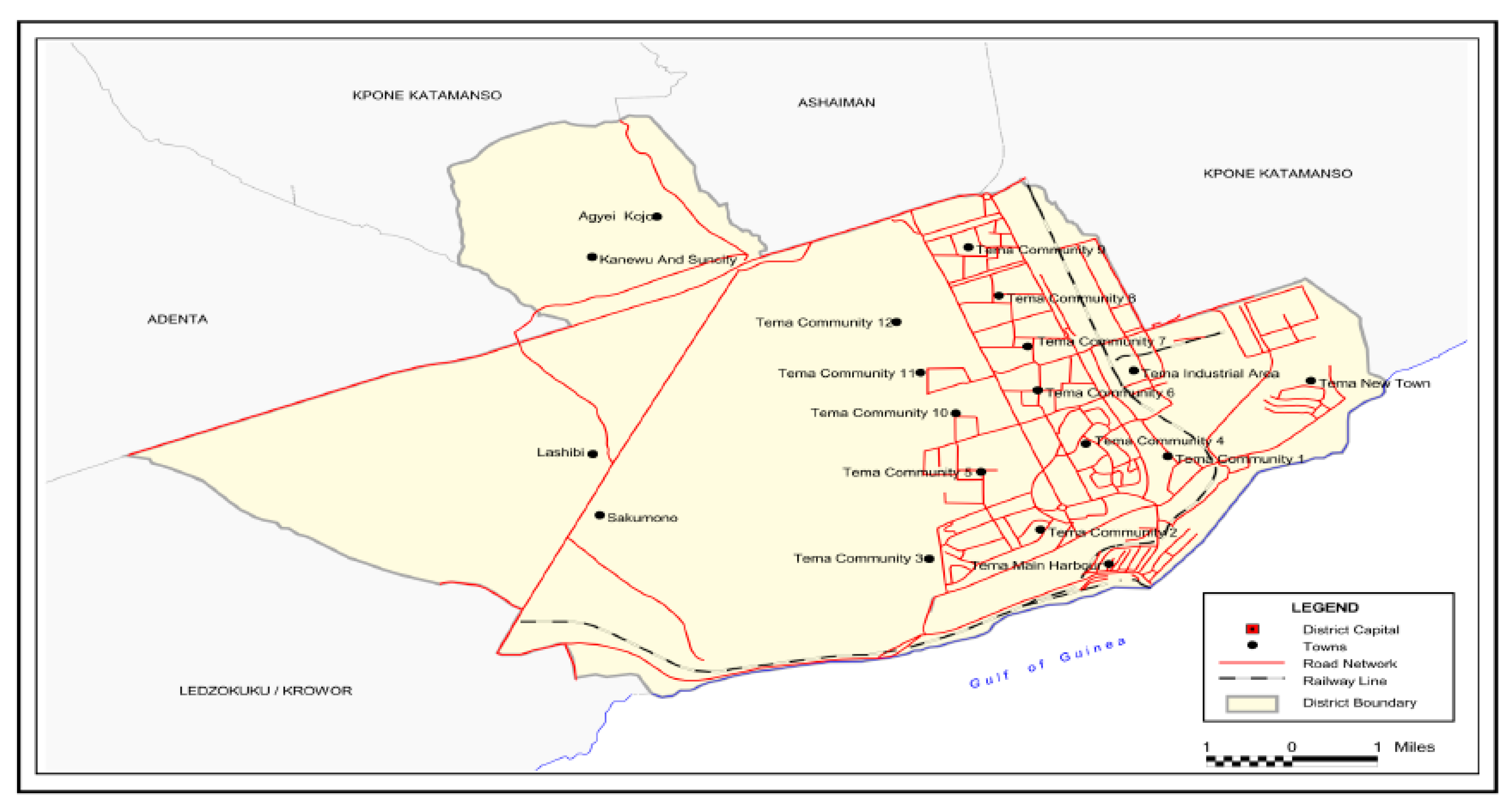
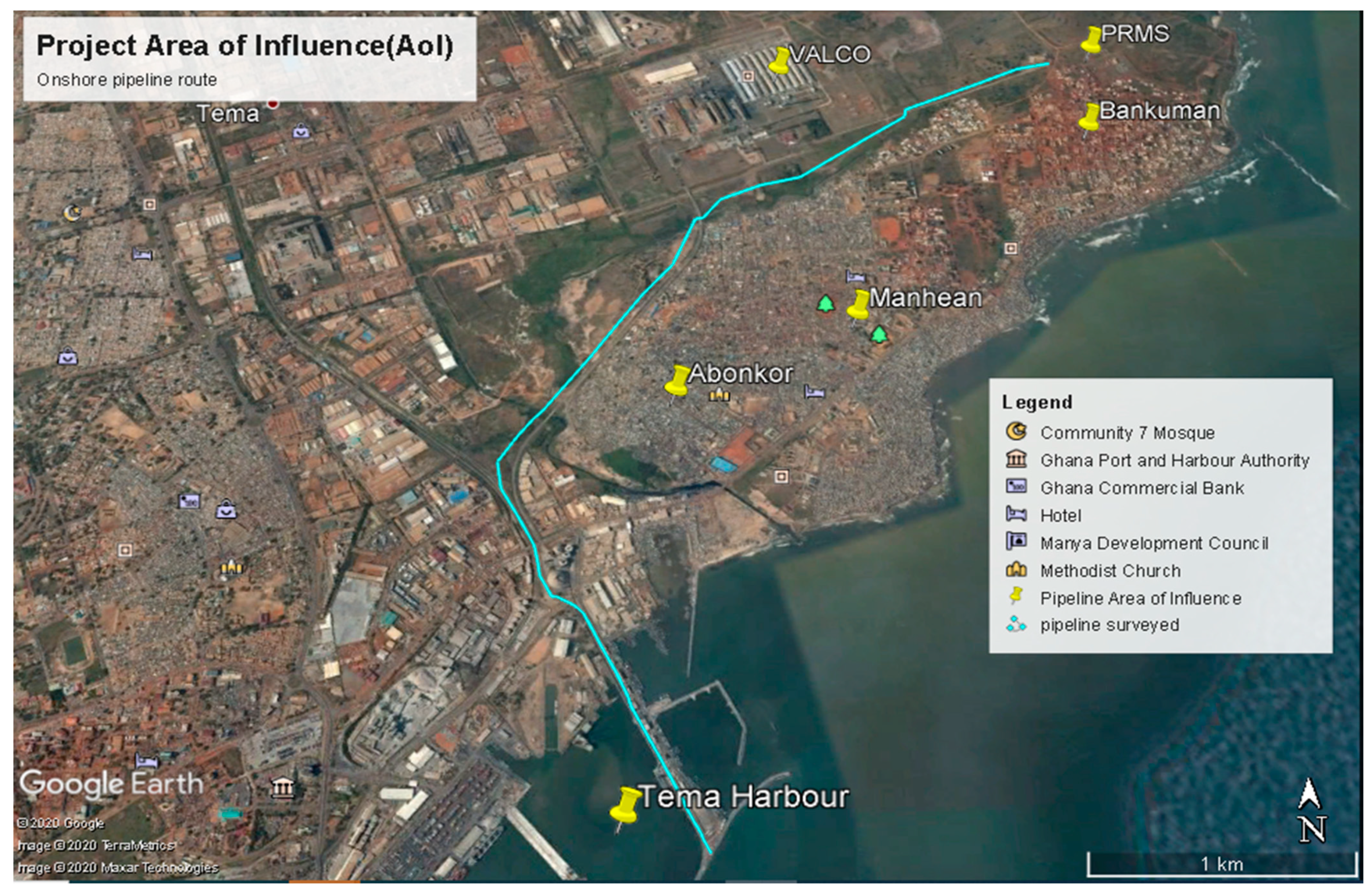
2.1. Study Area

Tema is the capital of Tema metropolitan district (see Figure 1) of the Greater Accra Region of Ghana. It is about 30 km from Accra, the nation’s capital. Tema is considered a heavily industrial area of Ghana in which most of Ghana’s industrial conglomerates are located. It is estimated to be home to over 1 million residents. Tema is a city on the Atlantic Ocean Coast, east of Ghana’s capital, and has one of Ghana’s main shipping harbor.

One major possible source of dust within the study period is the gas pipeline project laid through to a Pressure Reducing Metering Station (PRMS) at Kpong, 8 to 10 km away from the harbor. The project area of influence during the construction phase of the onshore pipeline was a 20 to 40 m pipeline right of way (RoW) for equipment/machinery and material space.

During laying of pipelines, dust from construction activities and moving of equipment may have been carried by wind to nearby receptors such as residential facilities of nearby local communities. The pipeline route goes along the Tema Oil Refinery (TOR) RoW within the port boundaries and then uses the Volta Aluminum Company (VALCO) RoW to the Volta River Authority (VRA) Header Station. The key communities along the route as evident in Figure 2 include; Abonkor, Manhean, and Bankuman, all within 10 km of the pipeline route.

2.2. Measurements

Continuous monitoring and measurement of particulate were carried out within the demarcated area to assess the impact of those ongoing activities. The sampling locations included the project area at the harbor (near the oil jetty), Abonkor, and Bankuman communities near the onshore pipeline and at the Valco hospital about 100 m from the pipeline route. The indicators selected and measured include TSP, PM₁₀ (less than 10 µm in aerodynamic diameter), and PM_2.5 (less than 2.5 µm in aerodynamic diameter) at four different locations along the pipeline route (8–10 km from the floating regasification unit to the pressure reducing metering station). Baseline value was obtained from the average of a four-week measurement of the PM and TSP before the study data collection commenced. Measurements were done day and night at sampling points about 100 m apart in a given location. Monitoring was conducted once a week during the day and at night with a sampling period of 24 h per location, for 36 weeks. The time interval used in calculating daytime averages was 8 to 12 h while that used for night-time was strictly 12 h.

Pollution classification was based on Ghana standards—GHA [28], International Financial Corporation—IFC guidelines [29,30], and baseline values. Throughout the study, IFC refers to total suspended particles or particulate matter (2.5 or 10) pollution reference to International Financial Corporation guidelines, and GHA refers to total suspended particles or particulate matter (2.5 or 10) pollution reference to Ghana standard guidelines. In addition, Base refers to average baseline (mean of four-week readings) measurement of the particulate matter and total suspended particles before the study data collection commenced.

In measuring dust (particulate matter), the CEL 712 Microdust Pro Kit equipment (Casella solutions, Sterling, MA, USA) were used. Size selective adaptors for PM₁₀ and PM_2.5 was fitted onto the instrument’s probe and loaded with a pre-weighted filter (PM₁₀ and PM_2.5 foams) into the cassette holder. The sampling pump was adjusted to provide an appropriate flow rate (3.5 L/min). A measurement auto range was selected; an averaging period of 1 to 60 s and a logging interval of 1 s to 60 min were selected. The instrument calculates and records the average dust concentration for the sampling period. After sampling, the sampling pump and the monitor’s measurement run were stopped, and values were noted.

For TSP, measurement was made by inserting an adaptor onto the instrument’s probe without loading. The sampling pump was adjusted to provide appropriate flow rate (3.5 L/min). A measurement auto range was selected; an averaging period of 1 to 60 s and a logging interval of 1 s to 60 min were selected. The instrument calculates and records the average dust concentration for the sampling period (3–4 h after which the next particulate matter is measured). The plots in Figure 3 shows some few extreme observations in the measured PM and TSP concentrations. Some of the monitoring sites selected by the random process fell into locations with unfriendly conditions such as unpaved roads and direct community settings. This could account extremely high values of dust concentrations and community interference with the monitoring process.

2.3. Quality Assurance

Before location measurement, the probe was purged with purge bellow to inject clean air into the chamber, to remove possible contamination that might have settled on the optical components inside the probe, and to adjust or set instrument zeroing. The Microdust Pro comes with an optical calibration insert. The calibration insert was inserted into the probe to establish the known instrument sensitivity (that is, to create stable and fixed scattering effect and signal level per factory calibration). The probe had a fitting for dust particle compactors or cells (sampling hole) at the mid-section where a specific particulate matter compactor was fixed to determine its concentration. One end of the probe was connected to a pump that sucked in from the probe inlet and the other end to a display/monitor that displayed measurement values. The screen was color-coded to ease navigation. Once a measurement started, it turned green or red when stopped. When taking the measurement, real-time instantaneous and average levels were shown and subsequently stored in the memory for later review and analysis.

2.4. Statistical Analysis

Data on PM_2.5, PM₁₀, and TSP covering the 36 weeks for the 4 selected locations were extracted from the instruments. The raw data were evaluated using multiple quality control measures to ensure they were within acceptable levels of data quality. Missing values for any pollutant were deleted (only 2 for PM_2.5). All other observations were found to be within the acceptable range. Averages were computed for the two observations (day and night) for each week after the quality assurance stage.

The generalized linear model was then applied to independently assess the overall variation characteristics of the concentration of PM_2.5, PM₁₀, and TSP within four exposed communities in the Tema metropolitan area of Ghana. In each model, the concentration of PM_2.5, PM₁₀, and TSP represented the dependent variable with the locations and weeks representing the fixed effect independent variables. The generalized linear models were extensions of the linear regression model [31,32,33] where the random elements were now allowed to belong to a one-parameter exponential family of distributions that includes the normal Gaussian distribution. Components the GLM as defined by [34].

• A response variable y = PM_2.5;
• Linear predictors $\eta =X\beta$ (here, X₁ = weeks, X₂ = locations);
• The distribution of y (exponential dispersion family);
• Link function $g\left(\mu \right)=\eta$ with $\mu =E\left(y\right)$;
• A prior weight $\raisebox{1ex}{$1$}\!\left/ \!\raisebox{-1ex}{$\varphi $}\right.$.

The goodness-of-fit assessment is similar to the residual assessment in the linear regression case, except that in the case of GLM’s, standardization of residuals is required. A closely related study [35] applied what they called the land use regression (LUR) models to analyze characteristics of NO₂ concentration by region using data from selected locations administrative units of urban and non-urban regions in South Korea. All data processing and statistical analysis were performed in R package version 3.5.3 (http://www.R-project.org/ (accessed on 13 April 2021).

3. Results

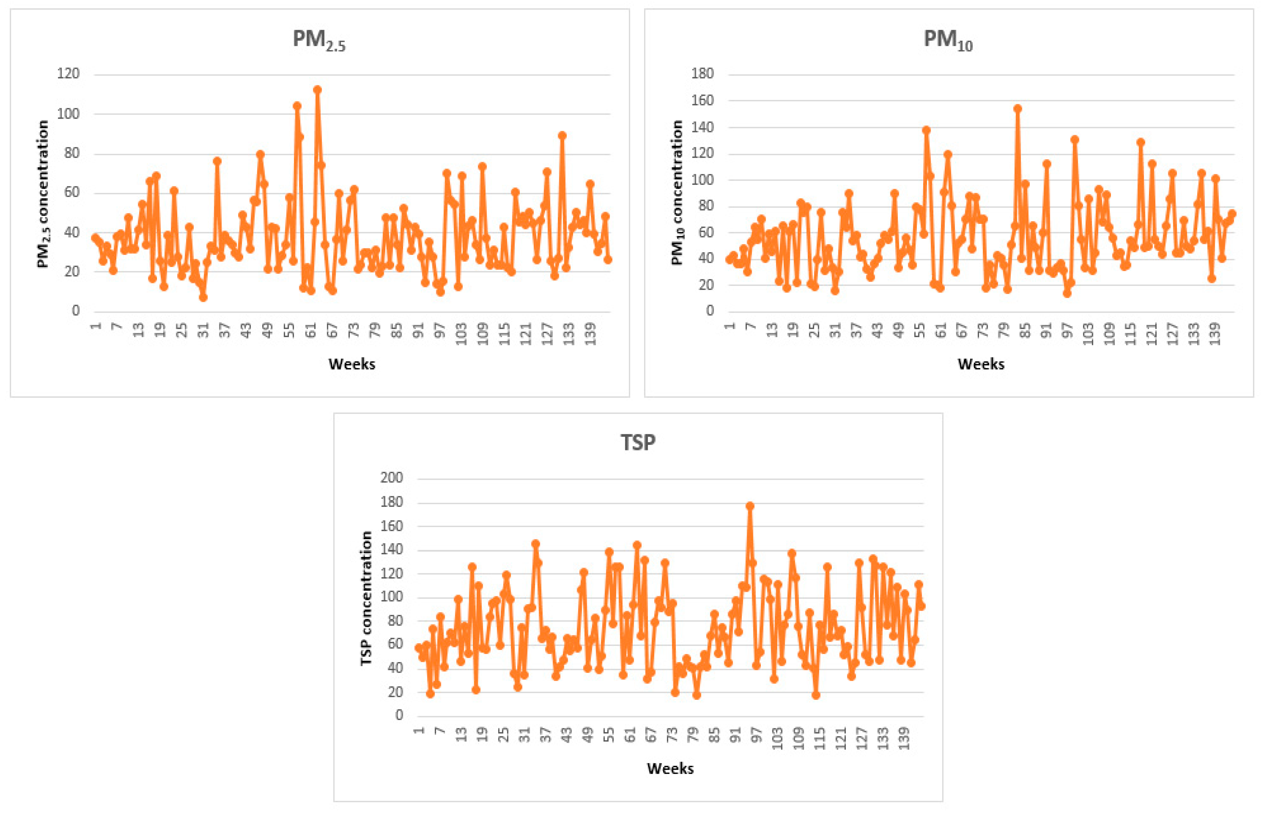
3.1. Descriptive Statistics

Table 1. Descriptive statistics (means in µg/m³).

Pollutants		Mean	N	Std. Deviation	Std. Error Mean
Pair 1	PM2.5 (Base)	38.85	144	20.7337	1.7278
	PM2.5	38.094	144	18.8788	1.5732
Pair 2	PM10 (Base)	69.425	144	12.4189	1.0349
	PM10	56.243	144	26.9193	2.2433
Pair 3	TSP (Base)	134.1	144	29.5117	2.4593
	TSP	75.122	144	33.1614	2.7634

presents descriptive statistics on the study variables by comparing the base readings with the readings of the study period. Mean of baseline PM_2.5 and actual PM_2.5 concentrations were 38.85 (s.e = 1.73) and 38.094 µg/m³ (s.e = 1.57), respectively. Per the IFC guidelines [29,30], an average weekly PM_2.5 concentrations value ≤ 25 µg/m³ is acceptable while an average weekly PM_2.5 value ≤ 35 µg/m³ is acceptable for the Ghana standards [28]. For these two benchmarks, the average weekly PM_2.5 value is clearly beyond the limits and gives an indication of PM_2.5 polluted environments.

Mean of baseline PM₁₀ and actual PM₁₀ concentrations were also found to 69.425 (s.e = 1.035) and 56.243 µg/m³ (s.e = 2.243), respectively. The IFC guidelines [29,30] put the acceptable limit at a weekly average of PM₁₀ ≤ 50 µg/m³ while an average weekly PM₁₀ value ≤ 70 µg/m³ is the acceptable limit by the Ghana standards [28]. For the IFC benchmark, the average weekly PM₁₀ values are clearly beyond the limits and give an indication of a PM₁₀ polluted environment. However, relying on the Ghana standards gives an indication of a PM₁₀ pollutant-free environment for our study area.

TSP average weekly values were found to be 134.1 (s.e = 2.459) and 75.122 µg/m³ (s.e = 2.763) for baseline and actual TSP, respectively. According to the Ghana standard benchmark [28], the average weekly TSP values were clearly beyond the limits (TSP ≤ 150 µg/m³) and provided an indication of a TSP-polluted environment before the study period, but a TSP pollutant-free environment throughout our study period.

3.2. Differences between Baseline Pollution Levels and Study Period Pollution Levels

A paired t-test was done to examine whether or not differences exist between baseline dust pollution levels and study period pollution levels. From

Table 2. Paired sample test.

Pollutant		Paired Differences					t	df	Sig.
		Mean	Std. Dev	Std. Error Mean	95% Confidence Interval of the Difference				(2-Tailed)
					Lower	Upper
Pair 1	PM2.5 (Base)	0.7563	24.9381	2.0782	−3.3517	4.8642	0.364	143	0.716
	PM2.5
Pair 2	PM10 (Base)	13.1823	29.3965	2.4497	8.34	18.0246	5.381	143	0.000
	PM10
Pair 3	TSP (Base)	58.9785	43.3274	3.6106	51.8414	66.1155	16.335	143	0.000
	TSP

, the results of the paired t-test indicate that no significant difference existed between baseline PM_2.5 pollution levels and study period PM_2.5 pollution levels [t(df = 143) = 0.364, p < 0.716]. Thus, for PM_2.5 concentration, although the average weekly baseline was higher (38.85 µg/m³) than that recorded over the study period (38.094 µg/m³), the difference is not statistically significant.

In the case of PM₁₀ concentration and TSP, the results indicated that there exists a significant difference in the baseline pollution levels and study period pollution levels (for PM₁₀: t(df = 143) = 5.381, $p<{10}^{-4}$; for TSP: t(df = 143) = 16.335, $p<{10}^{-4}$). Pollution levels for PM₁₀ concentration and TSP were significantly less over the study period than it was before the study.

3.3. Levels of Dust Pollution across the Four (4) Locations

The Chi-square test in

Table 3. Dust pollution across the selected locations base on the IFC and Ghana standards.

Pollutant	Location	No Pollution	Pollution	Chi-Square
PM2.5 (IFC)	Abonkor	7	29	0.499
	Bankuman	7	29
	Oil Jetty	11	25
	Valco Hospital	11	25
	Total	36	108
PM2.5 (GHA)	Abonkor	16	20	0.96
	Bankuman	15	21
	Oil Jetty	23	13
	Valco Hospital	23	13
	Total	77	67
PM10 (IFC)	Abonkor	15	21	0.391
	Bankuman	15	21
	Oil Jetty	19	17
	Valco Hospital	21	15
	Total	70	74
PM10 (GHA)	Abonkor	24	12	0.603
	Bankuman	27	9
	Oil Jetty	29	7
	Valco Hospital	27	9
	Total	107	37
TSP (GHA)	Abonkor	36	0	0.388
	Bankuman	36	0
	Oil Jetty	36	0
	Valco Hospital	35	1
	Total	143	1

examines whether or not there exists association between dust levels (categorized base on the standard benchmarks (IFC or GHA)) and study locations. Values of PM and TSP concentrations above the standards was categorized as pollution and those less or equal to the standard labeled as no pollution. It is obvious from the results that dust pollution was widespread across all four (4) locations studied (Chi-square: p < 0.499, based on PM_2.5_IFC; p < 0.96, based on PM_2.5_Ghana; p < 0.391, based on PM₁₀_IFC; p < 0.603, based on PM₁₀_Ghana; and p < 0.388, based on TSP_Ghana).

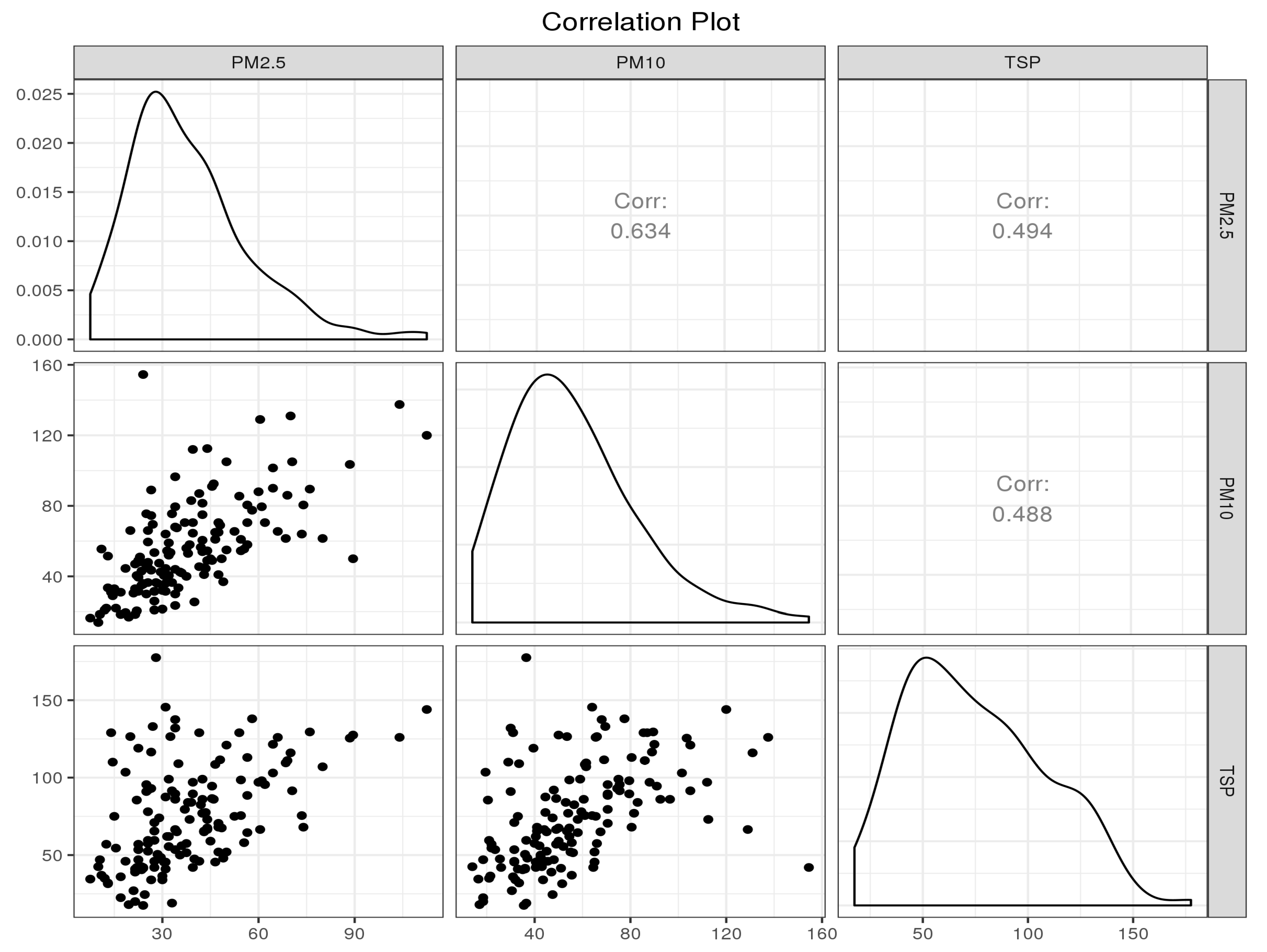
3.4. Correlation Analysis for PM_2.5, PM₁₀, and TSP

The inter-correlations among the pollutant (PM_2.5, PM₁₀, and TSP) were examined and reported in Figure 4. The plots on the leading diagonal represents a perfect correlation between each variable and itself. The first scatter plot represents the correlation between PM_2.5 (on the x-axis as seen on top) and PM₁₀ (on the y-axis as seen on right). The second plot shows the correlation between PM_2.5, (on the x-axis as seen on top) and TSP (on the y-axis as seen on right), while the final plot represents PM₁₀, (on the x-axis as seen on top) and TSP (on the y-axis as seen on right). PM_2.5 is found to have a strong direct correlation with PM₁₀ (r = 0.634) and a moderate direct correlation with TSP (r = 0.494). The relationship between PM₁₀ and TSP was also found to be moderate and direct (r = 0.488).

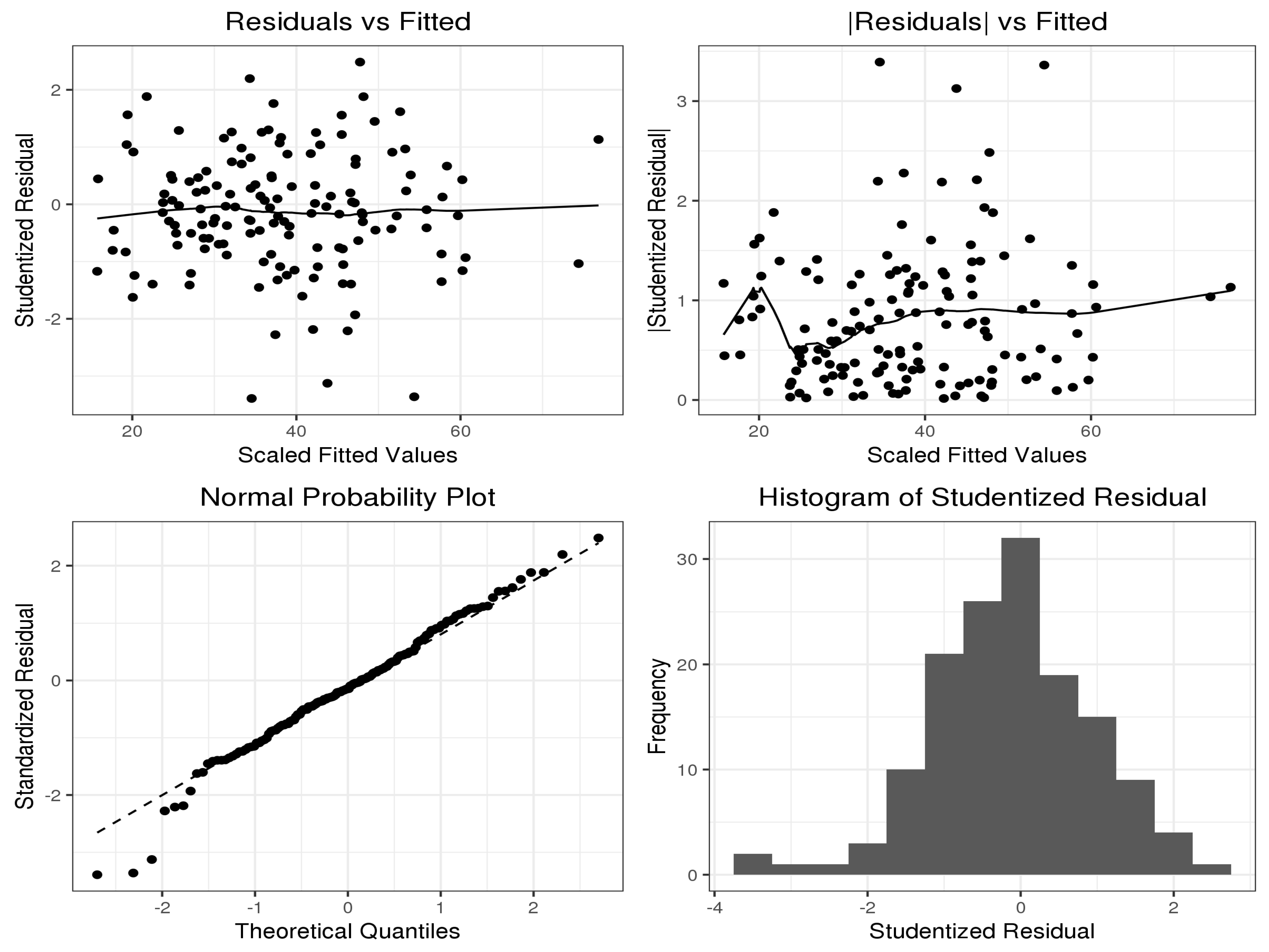
3.5. Model for PM_2.5

From the parameter estimates (

Table 4. Significant variable estimates for PM_2.5.

	Estimate	Std. Error	t Value	Pr (>|t|)
(Intercept)	4.08919	0.21929	18.64776	0.0000
1st week August 2020	−0.6199	0.29795	−2.08038	0.03992
3rd week August 2020	−0.6067	0.29795	−2.03608	0.04426
2nd week December 2020	−0.8911	0.29795	−2.9907	0.00347
3rd week December 2020	−1.0902	0.29795	−3.65894	0.0004
2nd week July 2020	−0.6781	0.29795	−2.27569	0.02489
4th week July 2020	−0.638	0.29795	−2.1413	0.03456
2nd week November 2020	−0.8431	0.29795	−2.8298	0.00558
3rd week January 2021	−0.9768	0.29795	−3.2784	0.00142
Oil Jetty	−0.2369	0.09932	−2.38514	0.01887
Valco Hospital	−0.2435	0.09932	−2.45161	0.01587

), the fitted Gamma GLM selected the following weeks as those that significantly received high levels of PM_2.5 concentration contributing significantly to PM_2.5 pollutions in the Tema metropolitan area. They include the second and third week of July 2020, the first and third week of August 2020, the second week of November 2020, the second and third week of December 2020, and, finally, the third week of January 2021. Again, of the four (4) locations, the oil jetty area and the VALCO hospital area were selected as the most PM_2.5 polluted areas within the Tema metropolitan area.

Model Diagnostics for PM_2.5

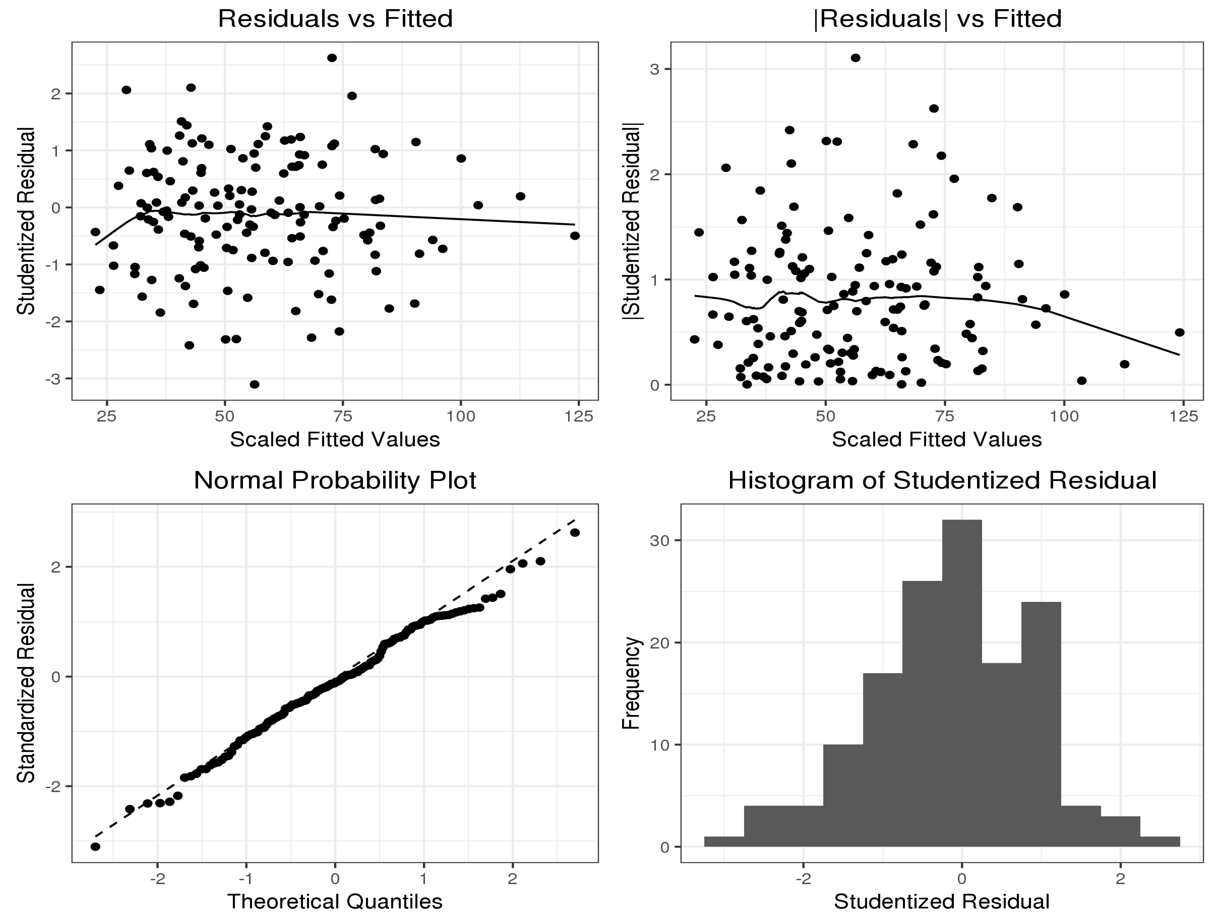
Model quality was assessed to ensure that PM_2.5 model has the quality of reliability and validity (goodness of fit). Figure 5 shows the model-checking plots for the PM_2.5 Gamma model. The diagnostic plots have several satisfactory features. The plot of residual vs. fitted (first plot) examines the accuracy of model specification. An accurately specified model has no form of a marked trend in the plot of residual vs. fitted [31,32,33]. From Figure 5, the running mean in the plot of residuals against fitted values shows no form of a marked trend indicating model prediction accuracy. The second plot (absolute residual vs. fitted) is used to examine whether or not variance function of the model is stable or trending. A suitable model should exhibit a flat trend of for the plot of absolute residuals vs. fitted. In our model, the plots of absolute residuals have a relatively stable slope indicating that errors are stationary and non-increasing. The third plot is the normal probability plot used together with the histogram of studentized residuals (fourth plot) to check the assumption of normality and possible effects of outliers in the data set. The normal plots show no discrepancy, while the histogram of the residuals shows a symmetric normal plot. These are very good indications of an appropriate and reliable model.

3.6. Model for PM₁₀

A Gaussian PM₁₀ Model was the best fit model as reported in

Table 5. Significant variable estimates for PM₁₀.

	Estimate	Std. Error	t Value	Pr (>|t|)
(Intercept)	4.40756	0.20017	22.01904	0.000
1st week August 2020	−0.7801	0.27198	−2.86811	0.00499
3rd week August 2020	−0.5408	0.27198	−1.98842	0.04937
2nd week December 2020	−0.9773	0.27198	−3.59332	0.0005
3rd week December 2020	−1.1339	0.27198	−4.16904	0.00006
1st week July 2020	−0.6976	0.27198	−2.56485	0.01174
2nd week July 2020	−0.6801	0.27198	−2.50064	0.01394
3rd week July 2020	−0.857	0.27198	−3.15107	0.00212
4th week July 2020	−0.711	0.27198	−2.61407	0.01026
2nd week November 2020	−0.709	0.27198	−2.60695	0.01046
3rd week October 2020	−0.7694	0.27198	−2.82879	0.0056
3rd week January 2021	−0.7766	0.27198	−2.85523	0.00518

. By the model, none of the four locations had significantly high levels of PM₁₀ pollution. The following weeks, however, were selected as those contributing significantly to PM₁₀ pollution in the Tema metropolitan area: first, second, third, and fourth week of July 2020, the first and third week of August 2020, the second week of November 2020, the second and third week of December 2020, the third week of October 2020, and finally, the third week of January 2021. By these results, all the weeks found to have received significantly high levels of PM_2.5 pollutions also showed significantly high PM₁₀ pollution.

Model Diagnostics for PM₁₀

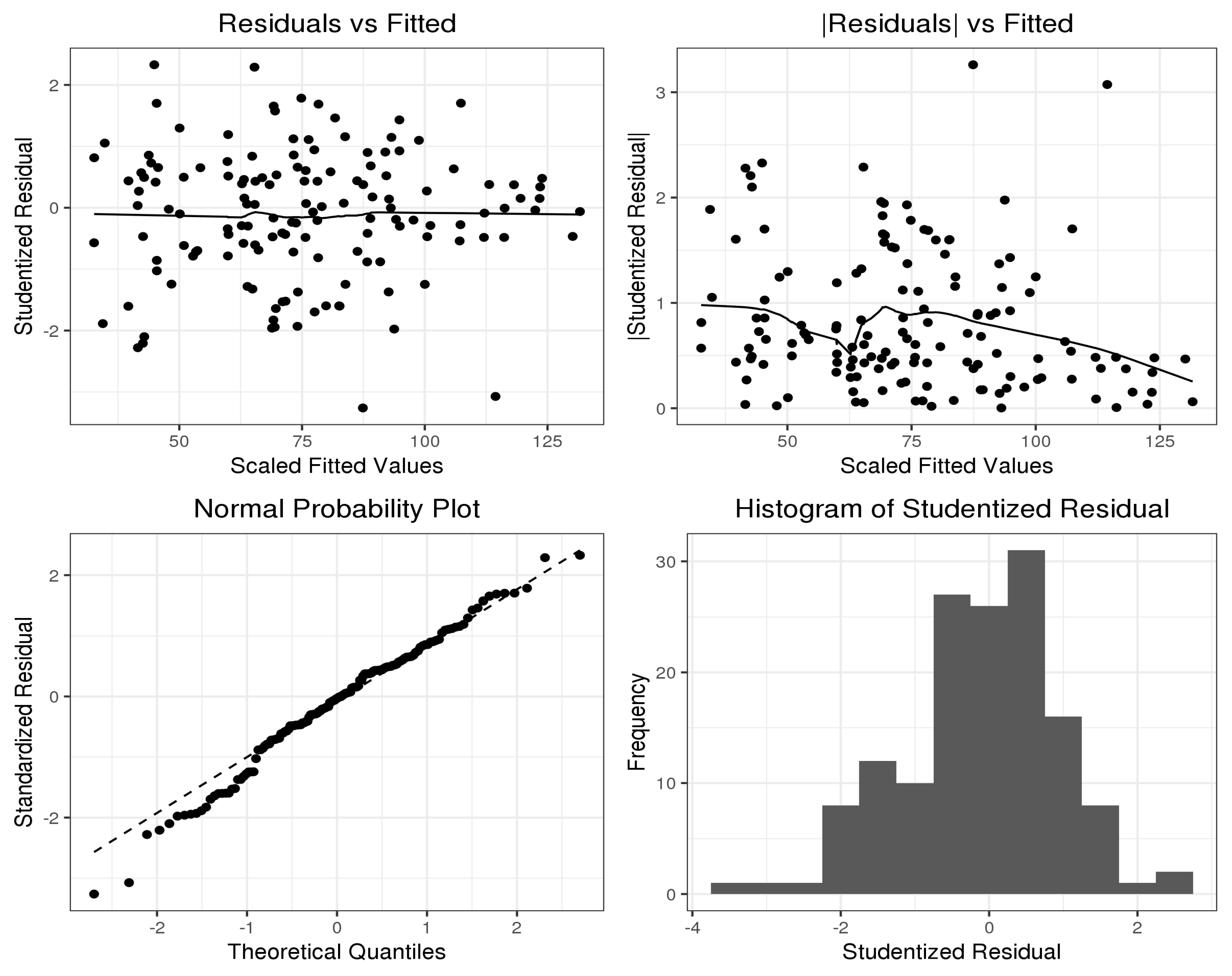
Just as has been explained for PM_2.5 model diagnostics, quality assessment for PM₁₀ Gaussian model also showed several satisfactory features as evident in Figure 6. The running mean in the plot of residuals against fitted values shows no form of a marked trend indicating model prediction accuracy. The plots of absolute residuals were shown sloping downwards, indicating that errors are stationary and decreasing. The normal plots showed no discrepancy while the histogram of the residuals showed a symmetric normal plot. These are very good indications of an appropriate and reliable model.

3.7. Model for TSP

A Gamma TSP model parameter as shown in

Table 6. Significant variable estimates for TSP.

	Estimate	Std. Error	t Value	Pr (>|t|)
(Intercept)	4.15834	0.1964	21.17298	0.0000
1st week August 2020	−0.60835	0.26685	−2.2797	0.02465
1st week December 2020	0.58142	0.26685	2.17879	0.03158
4th week November 2020	0.62502	0.26685	2.34219	0.02106
4th week February 2021	0.72145	0.26685	2.70354	0.008
December/January	0.66109	0.26685	2.47735	0.01483

also found none of the four locations to be significantly polluted by TSP. The first week of August runs through as the week found to have received significantly high levels of all the pollutants (PM_2.5, PM₁₀, and TSP) studied by this research. The weeks with exclusively high levels of TSP pollutions included fourth week of November 2020, first week of December 2020, the last week of December 2020 moving into first week of January 2021, as well as the fourth week of February 2021.

Model Diagnostics for TSP

Model quality assessment for TSP Gamma model, just as has been explained for PM_2.5 and PM₁₀ model diagnostics, also showed several satisfactory features as evident in Figure 7.

4. Discussion

Results from this study summarize the fact that some weeks’ records significantly high levels of dust pollution (PM_2.5, PM₁₀, and TSP) in a typical year. It was for instance revealed that all the weeks found to have received significantly high levels of PM_2.5 pollutions also showed significantly high PM₁₀ pollution. In fact, the first week of August runs through as the week found to have received significantly high levels of all the pollutants (PM_2.5, PM₁₀, and TSP) studied by this research. High levels of particulate matter in an environment illustrate the potential of macro-environmental exposures [24]. The use of the generalized linear models is new, and many studies are yet to explore its feature and flexibility in selecting useful variables in similar studies. However, the results of this study agree with a similar work that studies particulate matter in air quality research using different methods of analysis. In a related study, [4] collected PM_2.5 samples and observed that the highest average monthly concentrations occur in Winter (November to February) and become minimal during Summer (July–October).

The current study confirms the occurrence of high levels of dust pollutants in autumn and winter but differs from the summer findings. In Shi et al. [36], medium-volume air samplers were used to measure PM_2.5, PM₁₀, and TSP from January 2009 to March 2013 and found peak levels of these pollutants especially in January and December each year. It stands to reason from the above findings and commensurate agreements with previous related works that unfavorable weather conditions may be catalyzing high levels of pollution in the selected weeks. Low wind speed, low mixing heights, and low precipitation within the industrial enclave of the Tema metropolitan area become common from July to December. [4] made a similar observation for the Sichuan Basin in China. Low and stagnant atmospheric conditions highly impair the transportation and dispersion capacity of ambient air pollutants like PM_2.5, PM₁₀, and TSP [27].

The results also presented some spatial variations in the concentration of especially PM_2.5. The consideration of four (4) locations under this study is an improvement of a similar work by [37] where only one location was selected and monitored. The oil jetty area, as well as the VALCO hospital area, were the most severely affected by high levels of PM_2.5 pollutants. These two areas suffer from many of the immediate effects of construction and manufacturing activities within the Tema industrial enclave. Unlike other suburbs of Tema, the oil jetty and VALCO areas play host to many direct industrial pipes and heavy factory deposits. The selection of these two locations as heavily polluted is, therefore, a confirmation of many assertions of residents living around these areas.

The current study also found a strong to moderate correlation between the dust pollutants, especially PM_2.5 and PM_2.5. This confirms the statistical modeling findings to the effect that weeks found to have received significantly high levels of PM_2.5 pollutions also showed significantly high PM₁₀ pollution. Similar findings were evident in [24,38,39,40].

One major limitation of this study, as it is with most related studies is with the inability to collect data over a relatively long period and a wider number of locations. This may limit the generalizability of our findings to the selected locations and their immediate surrounding communities. Again, monitoring sites selected by the random process sometimes fall into locations with unfriendly conditions such as unpaved roads and direct community settings. This may lead to the measurement of extremely high values of dust concentrations and community interference with the monitoring process. In addition, weekly measurements could have been made daily but for the absence of resources and funding support. Future studies may be needed to cover a wider scope to model for cumulative exposure to PM_2.5, PM₁₀, and total suspended particles (TSP).

5. Conclusions

The current study used the generalized linear models (GLM) to monitor and assess the overall variation characteristics of the concentration of PM_2.5, PM₁₀, and total suspended particles (TSP) within four exposed communities in the Tema metropolitan area of Ghana. The study has selected some specific weeks and locations showing significantly high concentrations of PM_2.5, PM₁₀, and total suspended particles (TSP). Weeks found to have received significantly high levels of PM_2.5 pollutions also showed significantly high PM₁₀ pollution with the first week of August running through as the week found to have received significantly high levels of all three pollutants (PM_2.5, PM₁₀, and TSP) studied by this research.

The oil jetty and VALCO hospital area were worst affected by PM_2.5, as clearly revealed by this study. An important implication of this current study is residents of the locations considered in this study, as well as the general public, will be aware of the extent of exposure to PM_2.5, PM₁₀, and total suspended particles (TSP). Ultimately, this research hopes to spark up air quality concerns and form the basis for a well-coordinated air pollution prevention and control plan for the republic of Ghana. Further studies shall seek to examine the impact of environmental and other human behavioral factors on air quality.

References

1. Wang, H.; Dwyer-Lindgren, L.; Lofgren, K.T.; Rajaratnam, J.K.; Marcus, J.R.; Levin-Rector, A.; Levitz, C.E.; Lopez, A.D.; Murray, C.J.L. Age specific and sex-specific mortality in 187 countries, 1970–2010: A systematic analysis for the global burden of disease study 2010. Lancet 2012, 380, 2071–2094. [Google Scholar] [CrossRef]
2. Guan, D.B.; Su, X.; Zhang, Q.; Peters, G.P.; Liu, Z.; Lei, Y.; He, K. The socioeconomic drivers of China’s primary PM2.5 emissions. Environ. Res. Lett. 2014, 9, 024010. [Google Scholar] [CrossRef] [Green Version]
3. Lei, Y.; Zhang, Q.; He, K.B.; Streets, D.G. Primary anthropogenic aerosol emission trends for China, 1990–2005. Atmos. Chem. Phys. 2011, 11, 931–954. [Google Scholar] [CrossRef] [Green Version]
4. Wang, H.; Shi, G.; Tian, M.; Zhang, L.; Chen, Y.; Yang, F.; Cao, X. Aerosol optical properties and chemical composition apportionment in Sichuan Basin, China. Sci. Total Environ. 2017, 577, 245–257. [Google Scholar] [CrossRef]
5. Egyptian Environmental Impact Assessment on Egyptian Natural Gas Company (GASCO) PETROSAFE. 2007. Available online: http://www.eib.org/attachments/pipeline/20070088_nts_en.pdf (accessed on 25 February 2021).
6. Chen, L.D.; Gao, Q.C. Chance and Challenge for China on Ecosystem Management: Lessons from West to East Pipeline Project Construction. J. Hum. Environ. 2006, 35, 91–93. [Google Scholar] [CrossRef]
7. Tomareva, I.A.; Kozlovtseva, E.; Perfilov, V.A. Impact of Pipeline Construction on Air Environment. IOP Conf. Ser. Mater. Sci. Eng. 2017, 262, 12168. [Google Scholar] [CrossRef]
8. Ren, L.H.; Zhou, Z.E.; Zhoa, X.Y.; Yang, W.; Yin, B.H.; Bai, Z.W.; Ji, Y.Q. Source apportionment of PM10 and PM2.5 in Urban Areas of Chongqing. Res. Environ. Sci. 2014, 27, 1387–1394. [Google Scholar]
9. Song, N.; Xu, H.; Bi, X.H.; Wu, J.H.; Zhang, Y.F.; Feng, H.H.; Feng, Y.C. Source apportionment of PM2.5 and PM10 in Haikou. Res. Environ. Sci. 2015, 28, 1501–1509. [Google Scholar]
10. Mao, P.; Li, J.; Jin, L.; Qi, J. Evaluation on Effects of Construction Dust Pollution on Economic Loss. In Proceedings of the International Conference on Construction and Real Estate Management, Guangzhou, China, 10–12 November 2017. [Google Scholar] [CrossRef]
11. Rui, D.M.; Chen, J.J.; Feng, Y.C. Study on Source Apportionment for Ambient Air PM10 in Nanjing. J. Environ. Sci. Manag. 2008, 33, 56–58. [Google Scholar]
12. Anderson, J.O.; Thundiyil, J.G.; Stolbach, A. Clearing the air: A review of the effects of particulate matter air pollution on human health. J. Med. Toxicol. 2012, 8, 166–175. [Google Scholar] [CrossRef] [Green Version]
13. Xia, T.; Zhu, Y.F.; Mu, L.N.; Zhang, Z.F.; Liu, S.J. Pulmonary diseases induced by ambient ultrafine and engineered nanoparticles in twenty-first century. Natl. Sci. Rev. 2016, 3, 416–429. [Google Scholar] [CrossRef]
14. Franklin, B.A.; Brook, R.; Pope, C.A. Air pollution and cardiovascular disease. Curr. Probl. Cardiol. 2015, 40, 207–238. [Google Scholar] [CrossRef] [PubMed]
15. Hoet, P.H.M.; Brüske-Hohlfeld, I.; Salata, O.V. Nanoparticles—Known and unknown health risks. J. Nanobiotechnol. 2004, 2, 12. [Google Scholar] [CrossRef] [PubMed] [Green Version]
16. Olvera, H.A.; Garcia, M.; Li, W.-W.; Yang, H.; Amaya, M.A.; Myers, O.; Burchiel, S.W.; Berwick, M.; Pingtore, N.E. Principal Component Analysis Optimization of a PM2.5 Land Use Regression Model with Small Monitoring Network. Sci. Total Environ. 2012, 425, 27–34. [Google Scholar] [CrossRef] [PubMed] [Green Version]
17. Zou, B.; Luo, Y.; Wan, N.; Zheng, Z.; Sternberg, T.; Liao, Y. Performance comparison of LUR and OK in PM2.5 concentration mapping: A multidimensional perspective. Sci. Rep. 2015, 5, 8698. [Google Scholar] [CrossRef] [PubMed] [Green Version]
18. Yang, G.; Huang, J.; Li, X. Mining sequential patterns of PM2.5 pollution in three zones in China. J. Clean. Prod. 2018, 170, 388–398. [Google Scholar] [CrossRef]
19. Pope, C.A., 3rd; Thun, M.J.; Namboodiri, M.M.; Dockery, D.W.; Evans, J.S.; Speizer, F.E.; Heath, C.W. Particulate air pollution as a predictor of mortality in a prospective study of U.S. adults. Am. J. Respir. Crit. Care Med. 1995, 151, 669–674. [Google Scholar] [CrossRef]
20. Du, X.; Kong, Q.; Ge, W.; Zhang, S.; Fu, L. Characterization of personal exposure concentration of fine particles for adults and children exposed to high ambient concentrations in Beijing, China. J. Environ. Sci. 2010, 22, 1757–1764. [Google Scholar] [CrossRef]
21. Ahmed, C.M.S.; Jiang, H.; Chen, J.Y.; Lin, Y.-H. Traffic-Related Particulate Matter and Cardiometabolic Syndrome: A Review. Atmosphere 2018, 9, 336. [Google Scholar] [CrossRef] [Green Version]
22. Zhang, H.; Tripathi, N.K. Geospatial hot spot analysis of lung cancer patients correlated to fine particulate matter (PM2.5) and industrial wind in eastern Thailand. J. Clean. Prod. 2018, 170, 407–424. [Google Scholar] [CrossRef]
23. Leelossy, A.; Molnar, F.; Izsak, F.; Havasi, A. Dispersion Modeling of Air Pollutants in the Atmosphere: A Review. Open Geosci. 2014, 6, 257–258. [Google Scholar] [CrossRef]
24. Liu, Y.; Lan, B.; Shirai, J.; Austin, E.; Yang, C.; Seto, E. Exposures to Air Pollution and Noise from Multi-Modal Commuting in a Chinese City. Int. J. Environ. Res. Public Health 2019, 16, 2539. [Google Scholar] [CrossRef] [Green Version]
25. Lilic, N.; Cvjetic, A.; Knezevic, D.; Milisavljevic, V.; Pantelic, U. Dust and Noise Environmental Impact Assessment and Control in Serbian Mining Practice. Minerals 2018, 8, 34. [Google Scholar] [CrossRef] [Green Version]
26. Kesarkar, A.P.; Dalvi, M.; Kaginalkar, A.; Ojha, A. Coupling of the Weather Research and Forecasting Model with AERMOD for pollutant dispersion modeling. A case study for PM10 dispersion over Pune, India. Atmos. Environ. 2007, 41, 1976–1988. [Google Scholar] [CrossRef]
27. Yan, H.; Ding, G.; Li, H.; Wang, Y.; Zhang, L.; Shen, Q.; Feng, K. Field Evaluation of the Dust Impacts from Construction Sites on Surrounding Areas: A City Case Study in China. Sustainability 2019, 11, 1906. [Google Scholar] [CrossRef] [Green Version]
28. Ghana EPA. Annual Report 2015. Retrieved from Accra. 2016. Available online: http://www.epa.gov.gh/epa/sites/default/files/downloads/publications/2015%20Annual%20Report.pdf (accessed on 25 February 2021).
29. WHO. Air Quality Guidelines for Particulate Matter, Ozone, Nitrogen Dioxide and Sulfur Dioxide. Global Update 2006, WHO/SDE/PHE/OEH/06.02. 2006. Available online: https://apps.who.int/iris/bitstream/handle/10665/69477/WHO_SDE_PHE_OEH_06.02_eng.pdf?sequence=1 (accessed on 25 February 2021).
30. WHO. WHO’s Ambient Air Pollution Database-Update 2014. Retrieved from Geneva. Available online: https://www.who.int/phe/health_topics/outdoorair/databases/AAP_database_results_2014.pdf (accessed on 25 February 2021).
31. Sarpong, S.; Sarpong, A.; Lee, Y. A Model for Determining Predictors of the MUAC in Acute Malnutrition in Ghana. Int. J. Environ. Res. Public Health 2021, 18, 3792. [Google Scholar] [CrossRef] [PubMed]
32. Sarpong, S.A.; Avuglah, R.K.; Nsowah-Nuamah, N.N.N. Application of Joint Generalized Linear Models in Determining Physical Support Factors that Influence Crop Yield in Northern Ghana. Univers. J. Agric. Res. 2020, 8, 124–130. [Google Scholar] [CrossRef]
33. Lee, Y.; Nelder, J.A.; Pawitan, Y. Generalized Linear Models with Random Effects: Unified Analysis via H-Likelihood; CRC Press: Boca Raton, FL, USA, 2018. [Google Scholar]
34. Lee, Y.; Nelder, J.A. Double hierarchical generalized linear models (with discussion). J. R. Stat. Soc. Ser. C Appl. Stat. 2006, 55, 139–185. [Google Scholar] [CrossRef]
35. Ryu, J.; Park, C.; Jeon, S.W. Mapping and statistical analysis of NO2 concentration for local government air quality regulation. Sustainability 2019, 11, 3809. [Google Scholar] [CrossRef] [Green Version]
36. Shi, G.; Peng, X.; Liu, J.; Tian, Y.; Song, D.; Yu, H.; Feng, Y.; Russell, A.G. Quantification of long-term primary and secondary source contributions to carbonaceous aerosols. Environ. Pollut. 2016, 219, 897–905. [Google Scholar] [CrossRef] [PubMed]
37. Yan, S.; Wei, L.; Duan, Y.; Li, H.; Liao, Y.; Lv, Q.; Zhu, F.; Wang, Z.; Lu, W.; Yin, P.; et al. Short-Term Effects of Meteorological Factors and Air Pollutants on Hand, Foot and Mouth Disease among Children in Shenzhen, China, 2009–2017. Int. J. Environ. Res. Public Health 2019, 16, 3639. [Google Scholar] [CrossRef] [PubMed] [Green Version]
38. Fontes, T.; Li, P.; Barros, N.; Zhao, P. Trends of PM2.5 concentrations in China: A long term approach. J. Environ. Manag. 2017, 196, 719–732. [Google Scholar] [CrossRef] [PubMed]
39. Huang, J.; Deng, F.; Wu, S.; Guo, X. Comparisons of personal exposure to PM2.5 and CO by different commuting modes in Beijing, China. Sci. Total Environ. 2012, 425, 52–59. [Google Scholar] [CrossRef] [PubMed]
40. Suárez, L.; Mesías, S.; Iglesias, V.; Silva, C.; Cáceres, D.D.; Ruiz-Rudolph, P. Personal exposure to particulate matter in commuters using different transport modes (bus, bicycle, car and subway) in an assigned route in downtown Santiago, Chile. Environ. Sci. Process. Impacts 2014, 16, 1309–1317. [Google Scholar] [CrossRef]
Figure 1. Map of Tema metropolitan area (Source: Ghana Statistical Service GIS unit).
Atmosphere 12 00700 g001
Figure 2. Location of study area (source: Google Earth accessed in January 2020).
Atmosphere 12 00700 g002
Figure 3. Plots of PM2.5, PM10, and TSP measured values.
Atmosphere 12 00700 g003
Figure 4. Correlation plot for PM2.5, PM10, and TSP.
Atmosphere 12 00700 g004
Figure 5. Plot of PM2.5 Gamma model diagnostics.
Atmosphere 12 00700 g005
Figure 6. Plot of PM10 Gaussian model diagnostics.
Atmosphere 12 00700 g006
Figure 7. Plots of TSP Gamma model diagnostics.
Atmosphere 12 00700 g007