Venus Atmospheric Dynamics at Two Altitudes: Akatsuki and Venus Express Cloud Tracking, Ground-Based Doppler Observations and Comparison with Modelling ^†

Abstract

We present new results of our studies of zonal and meridional winds in both hemispheres of Venus, using ground- and space-based coordinated observations. The results obtained from telescope observations were retrieved with a Doppler velocimetry method. The wind velocities retrieved from space used an improved cloud-tracked technique based on the phase correlation between images. We present evidence that the altitude level sensed by our Doppler velocimetry method is approximately four kilometres higher (~4 km) than that using ground-tracked winds (using 380 or 365 nm). Since we often take advantage of coordinated space and ground observations simultaneously, this altitude difference will be very relevant in order to estimate the vertical wind shear at the related heights in future observation campaigns. We also explored a previous coordinated campaign using Akatsuki observations and its Ultraviolet Imager (UVI) at 283 and 365 nm filters, which showed that cloud-tracked winds showed a difference of about 10–15 ms⁻¹, as in the case of the comparison between the Doppler velocimetry winds and the 365 nm cloudtracked winds. The results’ comparison also strongly suggested that the cloud-tracked winds based on the 283 nm filter’s images were sensing at about the same atmospheric altitude level as the Doppler winds. The observational results were compared with the ground-to-thermosphere 3D model developed at the Laboratoire de Meteorologie Dynamique (IPSL-Venus General Circulation Model (VGCM)) and AFES-Venus General Circulation Model (GCM), at several pressure levels (and related heights). The analysis and results showed the following: (1) additional confirmation of the coherence and complementarity in the results provided by these techniques on both the spatial and temporal time scales of the two methods; (2) we noticed in the following that the results from the two different Akatsuki/UVI filters (283 and 365 nm) showed an average difference of about 10–15 ± 5 ms⁻¹, and we suggest this may be related to SO₂ atmospheric fluctuations and the particular conditions in the coordinated observing time window; (3) we present evidence indicating that, in the context of our observations, visible Doppler methods (highly self-consistent) seem to sense wind speeds at a vertical level closer to or within the range sensed by the UVI 283 nm filter images (again, in the context of our observations); (4) modelling predicted wind profiles suggests that the layers of the atmosphere of Venus sensed by the methods referred to in Point 3 differ by approximately four km in altitude (~4 ± 2 km) regarding the cloud-tracked winds retrieved using 365 or 380 nm images.

1. Introduction

Recent observations of Venus’ atmosphere by space missions like Akatsuki [1] and Venus Express (VEx) [2,3] and ground-based campaigns facilitated an unprecedented characterization of winds [4,5]. At the same time, they opened new scientific questions such as: What processes control the transition region (70–120 km) between the super-rotating zonal flow and day-to-night circulation? How does the interplay of planetary and small-scale waves control the circulation features? Which mechanism accelerates the atmosphere to its super-rotation state? Is the meridional flow [6,7] relevant to ignite this phenomenon? What is the behaviour of the Venus mesosphere’s vertical wind shear?

The Japanese space probe Akatsuki was launched in May 2010, but failed to enter orbit in December of the same year. Nevertheless, after orbiting the Sun for five years, it was placed in an elliptic orbit around Venus to finally begin its mission in December 2015 [8]. It is currently operational, and among all the instruments onboard, there is one worthy of reference for this work: the Ultraviolet Imager (UVI), a camera that takes images of the solar radiation reflected by the planet’s clouds. It has two narrow bandpass filters centred at two ultraviolet wavelengths: 283 nm sensing the absorption of the SO${}_2$ distributed at the cloud tops and above and 365 nm targeting unidentified ultraviolet-absorbent substances [1,9], as is the case of Venus Express (VEx) with the Visible and Infrared Thermal Imaging Spectrometer (VIRTIS-M) imaging at 380 nm. Akatsuki’s low orbital inclination (<10${}^{\circ }$) makes it more suitable to observe low latitudes from both hemispheres simultaneously and monitor atmospheric circulation at cloud top heights, from cloud-tracking techniques. Both Akatsuki filters sound the Venusian atmosphere at the cloud top level, and according to Horinouchi et al. [1], both filters sound different altitudes a few kilometres apart. This is suggested by the difference in westward wind velocities between the two filters (e.g., wind velocities obtained from 283 nm images were higher than those retrieved from 365 nm images).

Our group optimised and fine-tuned a Doppler technique tool to retrieve winds at Venus’ cloud top region (70 km) in the visible [4,6,10,11]. Since the Doppler velocimetry technique is based on solar light scattered on Venus’ dayside, the altitude of the retrieved horizontal velocities is where optical depth unity is reached. Based on photometry and polarization, Hansen and Hovenier [12] determined that cloud top altitude, in the visible range, is located at about 65–70 km, where an optical depth of unity ($\tau$ = 1) is reached. Kawabata et al. [13] indicated that this level is about 40 hPa in pressure and 70 km in altitude, based on a detailed analysis of Pioneer Venus OCPP UV and visible data. Using the depth of CO${}_2$ bands in VEx/VIRTIS-M combined with Venus Monitoring Camera (VEx/VMC) UV images, Ignatiev [14] stated that the optical depth of the cloud haze is nearly 0.6 at 40 hPa and varies as ${\lambda }^{-1.7}$, implying that a $\tau$ = 1 level is reached within one scale height of the clouds’ top roughly at 70 km in altitude. Fedorova et al. [15] using SPICAV/VEx (Spectroscopy for the investigation of the characteristics of the atmosphere of Venus) VIS-IR observations demonstrated that, for a fixed upper aerosol scale height for all latitudes, the cloud top altitude varies from 68 to 73 km at latitudes from 50${}^{\circ }$ S to 50${}^{\circ }$ N with an average of ±0.8 km based on CO${}_2$ bands in the range of 1.4–1.6 $\mathsf{\mu }$m.

At the cloud top, an unknown absorber is responsible for high contrast clouds at UV and visible wavelengths, which enables the cloud-tracking wind measurement technique [16]. Although some variability in the cloud top altitude is known [17], both the 365 nm filter Akatsuki/UVI and the 380 nm channel VEx/VIRTIS-M images track cloud features at the cloud top level, which is estimated at 68–71 km [14,15,18]. This coincidence allows, at first glance, comparing magnitudes and variability between ground-based Doppler velocimetry results and the ones from tracking of the UV marking methods. In particular, this allows the comparison between (i) Doppler velocimetry results from the Very Large Telescope (VLT) and the Ultraviolet and Visual Echelle Spectrograph (UVES) [11], the Canada-France-Hawaii Telescope (CFHT) and the high-resolution spectrograph Echelle SpectroPolarimetric Device for the Observation of Stars (ESPaDOnS) (Machado et al. [4], Machado et al. [6] and the present work) and the Telescopio Nazionale Galileo (TNG) and the High-Accuracy Radial velocity Planet Searcher for the Northern Hemisphere (HARPS-N) [7] and (ii) the results from UV cloud tracking (380 nm) as from VEx/VIRTIS-M (Machado et al. [4], Machado et al. [6], Sánchez-Lavega et al. [19], Hueso et al. [20], Hueso et al. [21] and the present work) and Akatsuki/UVI 365 nm filter cloud-tracked winds (Gonçalves et al. [7] and Horinouchi et al. [1]).

In this work, we present zonal and meridional wind flow results in both hemispheres of Venus using space-based observations obtained from Akatsuki’s space probe (Japan Aerospace Exploration Agency—JAXA) observations, namely observations taken with the UVI instrument (283 nm filter) in January 2017. We present, and compare, new and unpublished wind results from ground-based observations at Canada-France-Hawaii Telescope (CFHT, Hawaii, USA) with the high-resolution spectrograph ESPaDOnS (February 2014) and simultaneous coordinated observations obtained with space-based observations from Venus Express (ESA) and the instrument VIRTIS-M (380 nm).

We compare these new results with zonal and meridional wind flow results from Akatsuki/UVI (365 nm filter) from January 2017 [7]. We also compare with previous runs’ cloud-tracked and Doppler wind results [4,6,11]. The referenced previous sets of coordinated observations at Venus cloud tops were based on two complementary techniques: ground-based Doppler velocimetry and cloud-tracked winds using VEx/VIRTIS-M imaging at 380 nm. Cloud-tracked winds trace the true atmospheric motion also responsible for the Doppler–Fizeau shift of the solar radiation on the dayside by super-rotating moving cloud tops, with respect to both the Sun and the observer [4,6]. The results from this work are also compared with previous reference Venus atmosphere dynamical studies.

In the present work context, we show the latitudinal profile of the zonal wind retrieved with cloud-tracking techniques, using Akatsuki’s UVI observations in two different filters (283 and 385 nm). As described in Section 4.1, the observational results show clearly that they sound two different heights in the atmosphere. We highlight that in the context of the work of Gonçalves et al. [7], we used coordinated observations from TNG/HARPS-N (28–29 January 2017) and Akatsuki/UVI (365 nm images). The related retrieved winds showed, as in previous works, a consistent difference of about 10–15 ms${}^{-1}$. In the present work, we present cloud-tracked winds based on the Akatsuki/UVI 283 nm images from the same coordinated campaign and using the same cloud-tracking tool based on the phase correlation between images, as we did in our previous work [7]. The objective was to obtain wind results with the two complementary techniques (Doppler velocimetry and cloud tracking at 283 and 365 nm) in the same temporal window. Since the UVI 283 nm filter is sensitive to the SO${}_2$ atmospheric distribution, which is variable with time [1,22], it was important to compare the results from our previous work with the analyses we did in the scope of the present work using Akatsuki/UVI 283 nm. The cloud-tracked winds obtained in the framework of the present work using 283 nm Akatsuki/UVI images were higher by about 10–15 ms${}^{-1}$ than the ones obtained with the same tool, and in the same temporal window, but using 365 nm images [7]. Moreover, the cloud-tracked winds obtained from 283 nm images were consistent with the Doppler winds obtained with CFHT/ESPaDOnS coordinated observations, which strongly suggests that Doppler winds were sensing approximately the same atmospheric altitude level of Venus of 283 nm Akatsuki/UVI images obtained in the time interval of 26–31 January 2017.

We also present the comparison from these investigations with other Doppler winds obtained from previous campaigns: HARPS-N/TNG, ESPaDOnS/CFHT, and UVES/VLT. Zonal wind predictions at the cloud-level layer and at different levels of altitude seemed to be consistent with available measurements [6,7,23]. Finally, these results were validated with predictions from a ground-to-thermosphere 3D model, developed at the Laboratoire de Meteorologie Dynamique [24,25], at several pressure levels (and related heights).

2. Wind Determination Methods at the Cloud Top

2.1. Cloud-Tracking Method—Wind Retrieval with Akatsuki UVI and VEx/VIRTIS-M

From space, clouds’ features were tracked on image pairs obtained by the Akatsuki UVI operating in the ultraviolet range (283 nm filter) and with a temporal interval of ∼2 h. Ultraviolet images showed the highest contrast features, and the UV tracers were roughly located at about 65–70 km above the surface [18]. Venus Express cloud top wind measurements based on tracking using images taken with the VIRTIS instrument [19,20] followed the same method as the one described for retrieving cloud-tracked winds based on Akatsuki’s observations.

The cloud tracking method is a crucial technique to retrieve the wind profiles of Venus. Therefore, accurate image navigation and processing are required to allow clear observation of the movement of patterns on the clouds. For Akatsuki, as described by Gonçalves et al. [7], the original UVI images were navigated using SPICE kernels (NAIF - Navigation and Ancillary Information Facility) and were then processed in order to enhance brightness and contrast using unsharp mask filters. As for VEx/VIRTIS, the images are also navigated and processed [4] improving the S/N ratio and allowing cloud features to be better discerned. Both VEx/VIRTIS and Akatsuki processed images were then projected depending on the latitude values they covered, cylindrical or polar projections for low-latitude or high-latitude cloud features, respectively. This projection was done with an angular resolution compatible with the image that presented the worst spacial resolution [6].

The wind velocities were measured by tracking the displacement of several features on the observed cloud layer, by finding matching features in a pair of navigated and processed images, which in turn allowed us to determine the velocities of these cloud features and, at last, deduce the average velocity for a specific cloud layer of the Venusian atmosphere [4,7].

The following mathematical expressions were used for the calculation of the wind components for both Akatsuki and VEx/VIRTIS data:

$$u=(a+H)·cos\lambda ·\frac{\Delta \varphi }{\Delta t}·\frac{\pi }{180}$$

(1)

$$v=(a+H)·\frac{\Delta \lambda }{\Delta t}·\frac{\pi }{180}$$

(2)

Here, a is the radius of Venus, H is the height above the surface, $\varphi$ and $\lambda$ are the longitude and latitude in degrees and $\Delta$t is the time difference between the images (in seconds).

The error in time $\delta$t was considered to be quite small; consequently, the absolute errors for both components of the winds are given by the next expressions: $\delta u\approx \delta X/\Delta t$ and $\delta v\approx \delta Y/\Delta t$, following the general expressions given by Bevington et al. [26]. In the expressions mentioned, $\delta$X and $\delta$Y are absolute errors for the spatial displacement of the clouds [4].

The errors associated with both components of the cloud-tracked winds were calculated in the same way we did in Machado et al. [4]. As we did in our previous paper [4], the grids used for cloud tracking had a spatial resolution of $0.2^{\circ }$ (both in latitude and longitude), so that $\delta$X and $\delta$Y were about 21 km, thus implying wind speed measurements errors of the order of 5 ms${}^{-1}$ for both components of the wind.

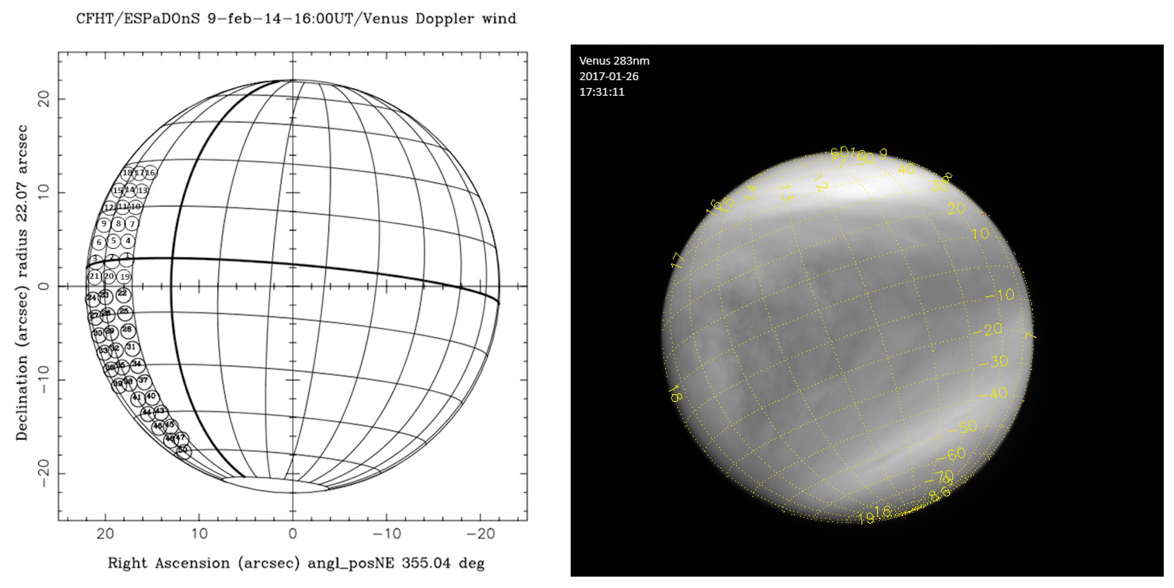
2.2. Doppler Wind Retrieval with CFHT/ESPaDOnS

ESPaDOnS was the visible spectropolarimeter used for these observations, covering wavelengths in the complete optical spectrum, from 370 to 1050 nm, collecting over 40 spectral orders in a single exposure, with a resolution of about 80,000 [27]. This instrument was used to provide direct wind velocity measurements using Fraunhofer lines scattered by Venus’ cloud tops. The emission from the warmer, deeper layer, by atoms and molecules of the solar atmosphere (H, S, Si, Fe, Ba, Mg, CN) [10], composes the Fraunhofer spectrum, which results from the absorption of solar continuum radiation scattered from Venus. The Doppler shift measured, in the single-scattering approximation, from the solar light scattered on Venus’ dayside, resulted in two instantaneous motions. The first one referred to the incoming radiation scattered in all directions, including the observer’s, is relative to the motion between the Sun and Venus’ upper clouds’ particles, resulting in a minimal Doppler velocity near Venus’ sub-solar point. The second one is relative to the motion between the observer and Venus’ clouds, resulting from Venus’ cloud particles’ topocentric velocity in the observer’s frame, which is minimal near Venus’ sub-terrestrial point [10]. The measured Doppler shift is the sum of those two terms. It therefore varies with planetocentric longitude. The Doppler shift vanishes at the half-phase angle meridian, where both terms cancel each other [4], and we used this meridian as the “zero-Doppler reference” to check for instrumental or calibration drifts. The Doppler velocities were modelled using two kinematical templates for the zonal wind: (1) solid rotation with v zonal = v (equator) × cos (latitude); (2) uniform retrograde velocity, v zonal = v (equator). Both models were explored within the latitudinal range 60${}^{\circ }$ S–60${}^{\circ }$ N. Once the best fit was obtained, we defined the acceptable domain at two-sigma and also tested alternative models, including the combination of both zonal and meridional circulations.

Since the finite angular size of the Sun on Venus’ dayside sky (its angular size is of about one degree) induces a spurious Doppler shift, the so-called Young effect [28], which is mandatory to control, we used the same approach as in Machado et al. [6] and Gonçalves et al. [7]. The protocol we used to evaluate and discard the Doppler shift due to the Young effect, as in previous works, was detailed in Gaulme et al. [29].

Previous techniques developed using high-resolution spectroscopy from the ground, to retrieve planetary wind measurements in the visible range [4,6,7,10,11,30,31,32,33], have addressed a fundamental problem in the maintenance of a stable velocity reference during acquisition [34]. Since the best accuracies achievable were of the order of 100 ms${}^{-1}$ (considering the dispersion law and instrumental uncertainties for single line shifts), they could not be considered an absolute reference rest frame. While for wind amplitude variations or latitudinal wind gradients on Venus, the measuring was done for the global wind circulation at the cloud tops, which was the order of 5 to 10 ms${}^{-1}$. One solution lies in the measurement of relative Doppler shifts between two sets of absorption lines. This technique is fundamentally based on the measuring and weighting of Doppler shifts between the solar Fraunhofer lines of two spectra—of solar radiation backscattered in the middle atmosphere—obtained simultaneously at different points of the slit.

2.3. Modelling

The predicted latitudinal profiles of zonal wind used in this work for comparison purposes were extracted from improved versions of the IPSL Venus General Circulation Model (IPSL-VGCM). This model has been used to investigate all regions of the Venusian atmosphere, as it covers the surface up to the thermosphere (150 km) [24,35,36,37].

Compared with the first version of the ground-to-thermosphere IPSL-VGCM published in Gilli et al. [24] (Gilli2017), the updated version described in Gilli et al. [25] (Gilli2021) includes several improvements in both the radiative transfer code and non-LTE (Local Thermodynamic Equilibrium) parameterization. Regarding the radiative part, a simplified cloud scheme (described in detail in Garate-Lopez et al. [36]) takes into account the latitudinal variation of the cloud structure based on Venus Express observations [38] and the lower haze heating rate, leading to a better agreement with in situ values of wind below the cloud deck (around 45 km altitude) by the Pioneer Venus probes [39]. A fine-tuning of non-LTE parameterization in Gilli2021 allows a better representation of the temperature profiles at altitudes above 100 km, such as those observed by the instrument on board the Venus Express, such as SPICAV (Spectroscopy for the Investigation of the Characteristics of the Atmosphere of Venus) and SOIR (SOlar Ocultation at Infrared). Furthermore, the horizontal resolution is increased from 7.5${}^{\circ }\times$ 5.625${}^{\circ }$ to 3.75${}^{\circ }\times$ 1.875${}^{\circ }$, resulting in qualitative changes to the circulation dynamics in the upper mesosphere and lower thermosphere, as explained in Navarro et al. [40]. We note that the vertical resolution of the IPSL-VGCM model is around 2 km at the altitudes sensed, on Venus’ atmosphere, in the context of the present work. Furthermore, consider that the altitudes attributed to model profiles are “approximate” altitudes, because the model outputs are in pressure. This means that, strictly speaking, the model profiles are not sensitive to lower than 2 km in the zonal wind profiles’ altitude variations.

We also took advantage of the Venus General Circulation Model (GCM) named AFES-Venus [41] in order to compare our zonal and meridional flow wind velocities with model-predicted results. The details of the model configuration were described in the work of Takagi et al. [42], in which three-dimensional structures of the thermal tide, Hadley’s cell-type meridional wind, and their contributions/relation with an overall meridional wind flow were elucidated.

3. Observations

CFHT/ESPaDOnS observations (see

Table 1. Orbital geometry and circumstances of ground-based observations: (1–2) Date/UT interval; (3–5) disk appearance; (6) sub-observer longitude and latitude (planetodetic); (7–9) observing conditions and geometry.

(1) Date	(2) UT	(3) Phase Angle $\mathsf{\Phi }$ (${}^{\circ }$)	(4) Ill.Fraction (%)	(5) Ang.Diam. (“)	(6)Ob-Lon/Lat (${}^{\circ }$)	(7) Airmass	(8) Seeing (“)	(9) PtSize (km)
8 February	15:50–16:43	126.96–126.93	19.93–19.96	45.13–45.11	13.92/−6.18	3.01–2.16	1.1–0.9	215
9 February	15:58–16:44	125.68–125.64	20.83–20.86	44.39–44.37	15.7/−6.1	3.08–2.12	1.0–0.8	218
10 February	15.54–16.39	124.44–124.39	21.73–21.76	43.66–43.64	17.51/−6.03	3.17–2.09	0.9–0.8	222

and Figure 1) were allocated to 8 February, 3:00–8:00 HST (13:00–18:00 UTC), 9 February, 3:00–8:00 HST (13:00–18:00 UTC), and 10 February, 3:00–8:00 HST (13:00–18:00 UTC), while VEx orbit planning indicated VIRTIS and VMC instruments during (3) Orbit 2851 (8 February, 18:00 UTC–February 9 4:00 UTC), (2) Orbit 2853 (10 February, 18:00 UTC–11 February, 5:00 UTC) and (3) Orbit 2854 (11 February, 19:00–23:00 UTC). Eventually, only Orbits 2851 and 2852 were used for synchronised VIRTIS-M UV cloud tracking at cloud tops with ground-based Doppler winds (see

Table 2. ESA Venus Express (VEx)/Visible and Infrared Thermal Imaging Spectrometer (VIRTIS-M) UV-visible channel for 380 nm observation circumstances: (1) orbit number; (2) VEx-VIRTIS hyperspectral images or "Qubes” pairs as defined by Cardesín [44]; (3) UT date; (4) time interval between selected image pairs; (5–6) corresponding latitude and local time range; the imaging spatial resolution varies between 15 km per pixel for polar latitudes and about 45 km per pixel for equatorial ones; (7) number of cloud tracers identified in image pairs.

(1) VEx Orbit	(2) Qubes Pairs	(3) Date (yyyy/mm/dd)	(4) Time Interval (min)	(5) Latitude Range	(6) Local Time Range	(7) Number of Points
2851	VV2851_01	2014/02/08	48	35${}^{\circ }$S–80${}^{\circ }$S	7 h–16 h	77
	VV2851_04
2853	VV2853_02	2014/02/10	48	5${}^{\circ }$S–70${}^{\circ }$S	7 h–10 h	23
	VV2853_05

).

3.1. Akatsuki/UVI and VEx/VIRTIS-M Description of Observations

3.1.1. Geometry of Observations with Akatsuki/UVI

Regarding the data from JAXA’s Akatsuki mission, a total of six days of observations were analysed, from 26–31 January 2017. Each day of observations had three images for the 283 nm UVI filter and the 365 nm filter, separated by approximately two hours each. The images available were processed and cloud tracked using combinations of 2 h spaced images, similar to the work of Gonçalves et al. [7]. In the framework of the present project, we analysed the 283 nm images of the temporal window from 26–31 January 2017. These images came from a coordinated observation campaign between our ground-based Doppler winds and Akatsuki’s UVI observations. Our goal was to use the same time images from the UVI’s two filters (283 and 365 nm) and analyse them using the same tool (cloud tracking with phase correlation between images). Besides the 365 nm images already studied in a previous work from our group [7], the same time 283 nm images had not yet been analysed by us. The relevance of studying here the 283 nm images from this period using the same tools we used before for the 365 nm images was the direct comparison of the retrieved wind fields and also the comparison with our Doppler winds. The analyses of the two UVI filters’ datasets in a simultaneous temporal period were mandatory, since the 283 nm filter is sensitive to the atmospheric SO${}_2$ distribution, which is highly variable, both spatially and temporally [1,22,43], and in the scope of the present work, we intended to address the difference in altitude sensed by the two UVI’s filters and compare them with the altitude sensed by our Doppler winds. In the following, we take advantage of Venus’ atmospheric GCM in order to proceed to the described altitude comparison.

Table 3. Image list from Akatsuki observations, from 26–31 January 2017, of Venus with the 283 nm Ultraviolet Imager (UVI) filter: (1) date and time in UTC; (2) mean resolution in deg/px; (3) mean resolution in km/px; (4) latitude range of Venus’ visible disk; (5) local time range of Venus’ visible dayside; (6) distance between VCO and Venus in km; (7) Venus’ apparent angular diameter in degrees.

(1) Date and Time UT	(2) deg/px	(3) km/px	(4) Latitude	(5) Local Time	(6) Distance to Venus (km)	(7) Venus’ Diameter (deg)
26-01-2017 17:31:11	0.360	38.462	72${}^{\circ }$N–88${}^{\circ }$S	7:30–18:00	138,938	5.05
26-01-2017 19:31:11	0.391	41.772	72${}^{\circ }$N–88${}^{\circ }$S	7:30–18:00	150,090	4.68
26-01-2017 21:31:12	0.420	44.859	72${}^{\circ }$N–88${}^{\circ }$S	7:30–18:00	160,630	4.37
27-01-2017 17:01:11	0.542	57.921	75${}^{\circ }$N–85${}^{\circ }$S	8:00–18:00	241,265	2.91
27-01-2017 19:01:11	0.556	59.377	75${}^{\circ }$N–85${}^{\circ }$S	8:00–18:00	247,863	2.83
27-01-2017 21:01:10	0.569	60.767	75${}^{\circ }$N–85${}^{\circ }$S	8:00–18:00	254,218	2.76
28-01-2017 18:01:11	0.679	72.473	75${}^{\circ }$N–85${}^{\circ }$S	8:30–18:00	308,616	2.27
28-01-2017 20:01:11	0.686	73.349	75${}^{\circ }$N–85${}^{\circ }$S	8:30–18:00	312,782	2.24
28-01-2017 22:01:11	0.694	74.151	75${}^{\circ }$N–85${}^{\circ }$S	8:30–18:00	316,792	2.21
29-01-2017 18:51:10	0.754	80.543	75${}^{\circ }$N–85${}^{\circ }$S	9:00–18:00	350,098	2.00
29-01-2017 20:51:10	0.758	80.983	75${}^{\circ }$N–85${}^{\circ }$S	9:00–18:00	352,541	1.99
29-01-2017 22:51:10	0.762	81.368	75${}^{\circ }$N–85${}^{\circ }$S	9:00–18:00	354,861	1.98
30-01-2017 18:01:11	0.785	83.844	75${}^{\circ }$N–85${}^{\circ }$S	9:15–18:00	371,060	1.89
30-01-2017 20:01:10	0.785	83.862	75${}^{\circ }$N–85${}^{\circ }$S	9:15–18:00	372,142	1.88
30-01-2017 22:01:11	0.786	84.023	75${}^{\circ }$N–85${}^{\circ }$S	9:15–18:00	373,111	1.88
31-01-2017 17:21:10	0.785	84.023	70${}^{\circ }$N–80${}^{\circ }$S	9:50–18:00	376,770	1.86
31-01-2017 19:21:09	0.784	83.817	70${}^{\circ }$N–80${}^{\circ }$S	9:50–18:00	376,561	1.86
31-01-2017 21:21:09	0.783	83.700	70${}^{\circ }$N–80${}^{\circ }$S	9:50–18:00	376,241	1.86

shows the characteristics and more details of each image used.

All the UVI images were navigated using an observation geometry system developed by NASA’s Navigation and Ancillary Information Facility (NAIF) called SPICE and were then processed in order to improve the signal-to-noise ratio. This was done by using a semi-automatic method, as described in Gonçalves et al. [7]. The images were also projected according to the latitudes sounded, polar projection for images with high latitudes towards the polar region and cylindrical projection for images covering latitudes closer to the equator.

3.1.2. Geometry of Observations with VEx/VIRTIS-M

The VEx/VIRTIS’ images used were selected from two Venus Express orbits (Orbit Number 2851 and Orbit Number 2853 from 8–10 February 2014, respectively), and a pair of QUBE images was used for each orbit. The images in each pair were separated by a time interval of 48 min and covered dayside longitudes on Venus’ southern hemisphere. Table 2 shows the specifics of the images used.

Similar to Akatsuki’s data explained above, the Vex/VIRTIS images were also navigated and processed to improve the signal-to-noise ratio followed by polar or cylindrical projection depending on whether the latitudes analysed were closer to the south pole or the equator [4].

3.2. CFHT/ESPaDOnS Observations

On February 2014, Venus was moving towards its maximum elongation, coming from its inferior conjunction in January of the same year. During observations between 8 and 10 February 2014, Venus was at a phase angle of 127–124${}^{\circ }$ (see Table 1), where it was possible to analyse the sub-solar meridian, the sub-terrestrial meridian and the half-phase angle meridian (HPA), in sequence from ground observations on the illuminated side of the morning terminator of the planet (Figure 1). The observed disk of Venus had a surface brightness of 1.37–1.39 (mag/arcsec) and an apparent magnitude of −4.89, and its illuminated fraction ranged from 19.9–21.8% at an angular diameter of 45.13–43.64 arcsec.

The observing strategy was to displace the spectrograph’s entrance fibre along with points on the dayside hemisphere (see Figure 1). Exposure times were adjusted at t = 3 s to obtain an S/N of 400–600 on the continuum and avoid saturation.

Table 4. Scanning sequences on Venus’ dayside hemisphere using CFHT/ESPaDOnS during the 8–10 February 2014 observing run: (1) sequence number; (2) location on disk; (3) UT time interval; (4) points’ acquisition order; (5) exposure repetition: each point is acquired 3 times to check for internal consistency.

(1) Sequence number	(2) Location	(3) Time Span (UT)	(4) Points Order	(5) Exposure Repetition
8 February 2014
$\left[1\right]$	S lat 10${}^{\circ }$	15:50–15:57	23-24-23-22-23	3×
$\left[2\right]$	S lat 15${}^{\circ }$	16:01–16:07	23-27-26-25-23	3×
$\left[3\right]$	S lat 10–20${}^{\circ }$	16:10–16:21	23-30-29-28-24-23	3×
$\left[4\right]$	S lat 25${}^{\circ }$	16:24–16:29	23-33-32-31-23	3×
$\left[5\right]$	S lat 30${}^{\circ }$	16:33–16:37	23-36-35-34-23	3×
$\left[6\right]$	S lat 35${}^{\circ }$	16:41–16:43	23-39-23	3×
9 February 2014
$\left[7\right]$	S Lat 25${}^{\circ }$	15:58–16:06	23-33-32-31-31-23	3×
$\left[8\right]$	S lat 30${}^{\circ }$	16:09–16:14	23-36-35-34-23	3×
$\left[9\right]$	S lat 25–35${}^{\circ }$	16:17–16:24	23-39-38-37-33-23	3×
$\left[10\right]$	S lat 40${}^{\circ }$	16:30–16:32	23-41-40-23	3×
$\left[11\right]$	S lat 45${}^{\circ }$	16:35–16:37	23-44-43-23	3×
$\left[12\right]$	S lat 50${}^{\circ }$	16:39–16:41	23-46-45-23	3×
$\left[13\right]$	S lat 25–55${}^{\circ }$	16:43–16:44	23-48-33-23	3×
10 February 2014
$\left[14\right]$	Equator	15:54–16:05	23-3-3-2-1-23	3×
$\left[15\right]$	N lat 5${}^{\circ }$	16:08–16:15	23-6-5-5-4-23	3×
$\left[16\right]$	Equator –N lat 10${}^{\circ }$	16:18–16:29	23-9-9-8-7-3-23	3×
$\left[17\right]$	N lat 15${}^{\circ }$	16:33–16:39	23-12-11-11-10-23	3×

presents the scanning routine on Venus’ dayside hemisphere during the observing run on 8–10 February 2014. Weather conditions did not impose any relevant constraints during the observations. However, observation times were limited due to Venus being on the leading side of the Sun, and some observations were performed shortly before sunrise. The sequence number enumerated each full sequence observed, each beginning and ending with the null-Doppler reference point 23. The location on the disk (Column 2) indicates the latitude band where each observing sequence took place by manually guiding the telescope to each offset position using the telescope controls (TCS) and a template of the pointing sequence dimensioned to the instrument’s guiding camera display. Manual guiding towards each point took approximately 2 min (3 s exposures followed by 40 s of detector readout).

Some observational exposures were discarded from the analysis either for their lower S/N and/or limb or high solar zenith angle (SZA) geometry, their drifting away from the position, a telescope manual tracking issue or seeing or weather issues such as passing cirrus. Nevertheless, the overall number of discarded exposures was lower than 10% from the total.

The observer manually corrects the tracking errors during the overhead time between sky exposures. The estimated combined pointing and tracking error was less than 0.4 arcsec, of the order of seeing conditions and within the ESPaDOnS FOV projected diameter of 1.6 arcsec on Venus. Note that this upper limit is equal for all points as the quality of guiding is independent of the solar zenith angle on Venus.

In addition to the coordinate observing effort with the VEx space probe, the choice of observing dates offered a compromise on the need to maximize the apparent angular diameter of the disk of Venus, thus the spatial resolution of the disk, even if the illuminated fraction is small (≈20${}^{\circ }$).

4. Cloud-Tracking Results

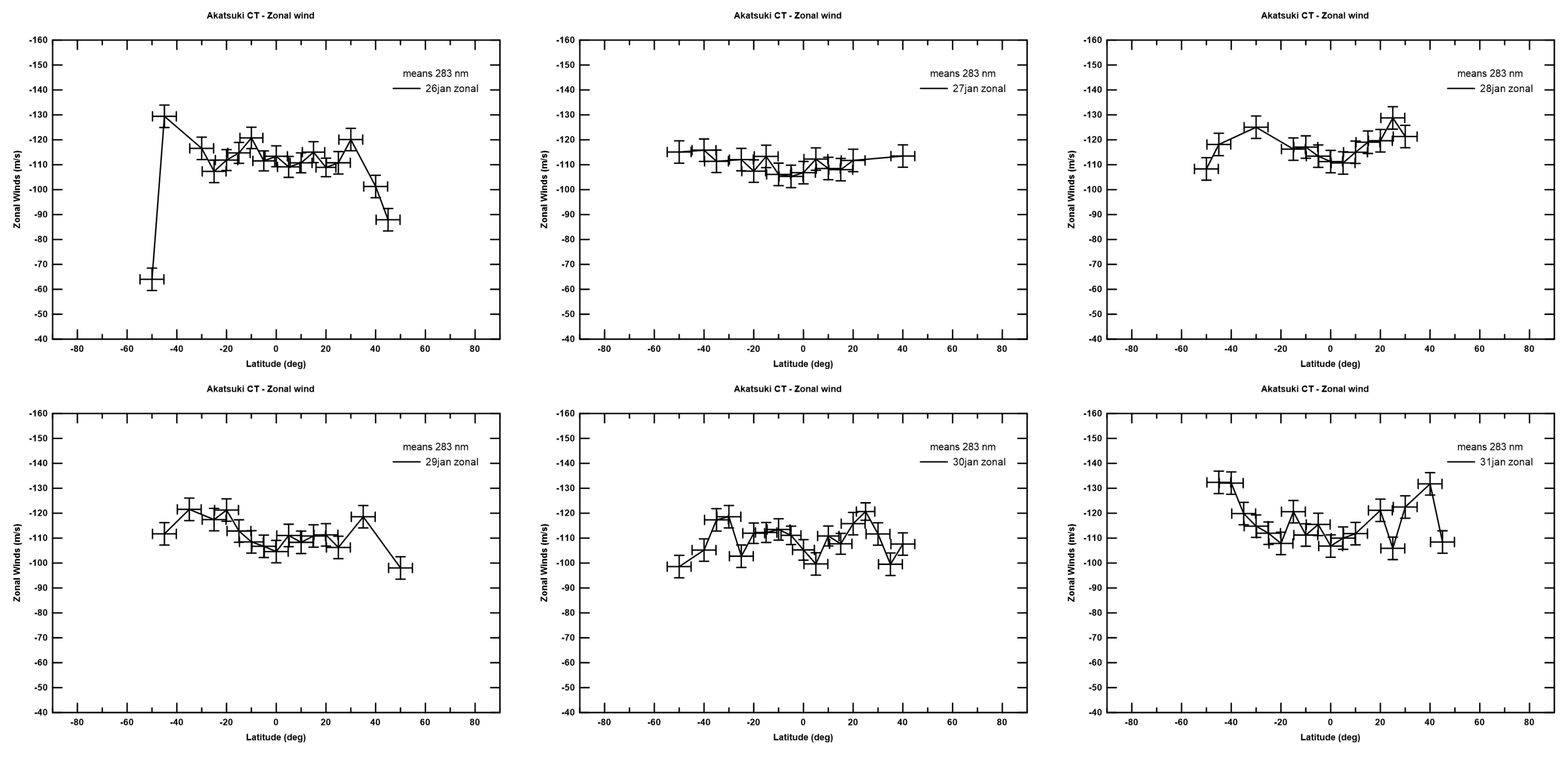
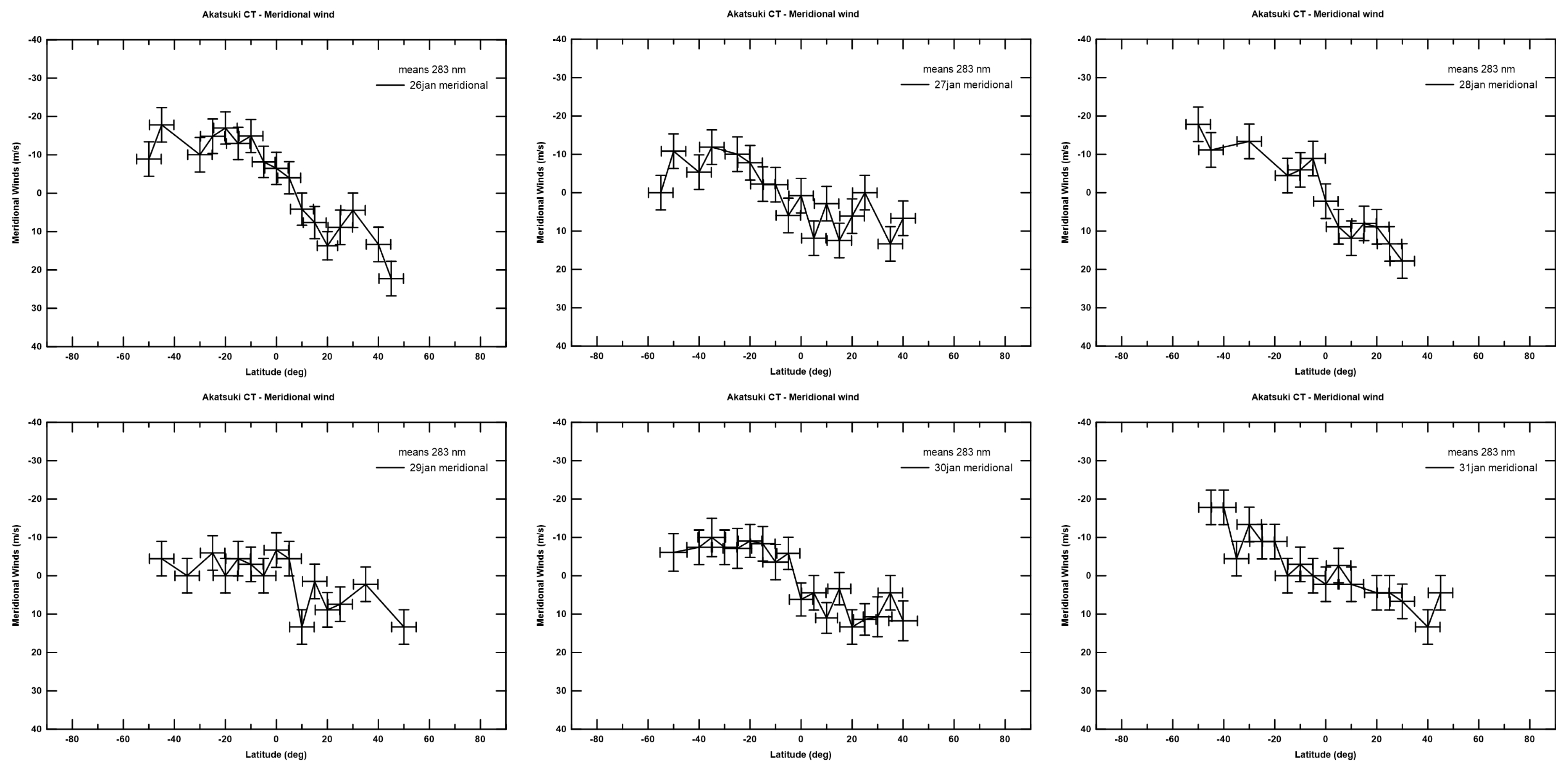
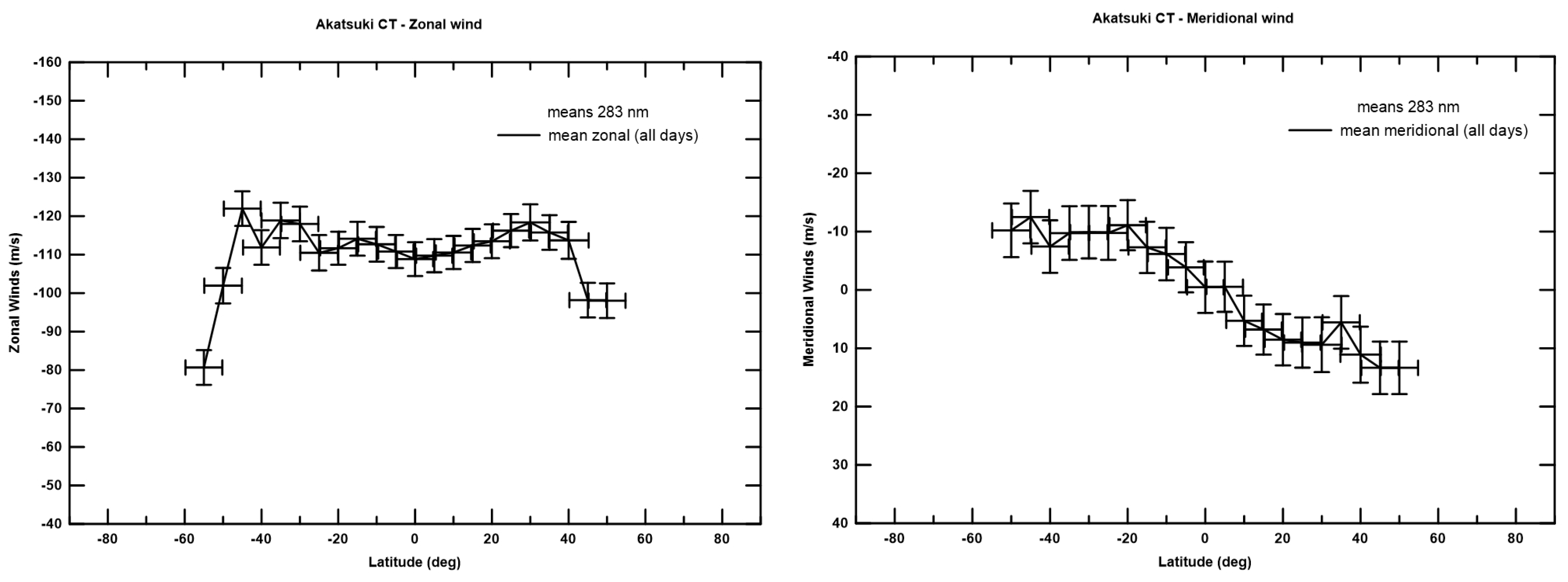
4.1. Akatsuki UVI 283 nm Filter Wind Velocities’ Results

After retrieving wind velocities based on Akatsuki/UVI observations, described in the previous section and using the method referred to in the techniques’ description-related section, we produced daily latitudinal wind profiles that are shown in the next figures (Figure 2 and Figure 3). We computed wind velocities based on the Akatsuki/UVI 283 nm filter, both zonal and meridional wind components, and then, we compared them with the other 365 nm UVI filter.

Figure 2 presents the daily latitudinal zonal wind profile, based on a weighted average on all the zonal winds retrieved each day, with a binning of 5${}^{\circ }$ in latitude.

As in the case of Gonçalves et al. [7], where we presented cloud-tracked winds based on 365 nm Akatsuki/UVI images, the method’s uncertainties, related to this work, were essentially due to the spatial resolution of the images even though the time error was relatively negligible. The absolute errors for the spatial displacement of the clouds were of the order of 38 to 85 km, which implies errors of wind velocity measurements of around 5 to 10 ms${}^{-1}$, and were a function of the images’ resolution, for both components of the wind (again, the error associated with the time measured at each image acquisition was negligible).

The weighting coefficients used to obtain the weighted average of zonal wind velocities’ in each latitude band were the inverse of the variance associated with the uncertainty in retrieving each velocity measurement. These errors were described in the previous paragraph (see Machado et al. [6] for more details concerning the process of estimating errors). However, regarding the velocity of zonal winds, we present (Figure 4, left panel) the mean zonal velocity in a latitudinal profile of the full observation campaign of February 2014 considering a 5${}^{\circ }$ binning in latitude.

The first striking reading we obtained from these results (from the 283 nm Akatsuki UVI filter of zonal wind) was that their magnitude was greater by about 10–15 ± 5 ms${}^{-1}$ than the ones retrieved with the 365 nm filter during the same period [7]. We note that the two datasets came from almost the same period for each day of the observational run. The second striking reading, which can be seen in Figure 4, was that zonal winds were roughly consistent between each day’s measurements, showing an almost uniform velocity up to 50${}^{\circ }$ N-S, where a maximum was reached, and a steep decrease at higher latitudes.

The measured zonal wind in midlatitudes was of the order of 115–120 ± 5 ms${}^{-1}$ for the period of observations presented here. Noticeable as well was a general daily variability—both spatial and temporal—of about 5–10 ms${}^{-1}$. Between the 28th and 29th zonal wind panels, it is clear that there was a ∼5 ms${}^{-1}$ higher velocity among the latitude ranges of 30–40${}^{\circ }$ in the southern hemisphere.

The evidence for a north-south asymmetry shown in the 365 nm filter images, in the same period, in Gonçalves et al. [7] and also in Horinouchi et al. [1] (also using Akatsuki UVI images) was not clear in the results that we present here.

When we considered the latitudinal mean zonal wind profile (Figure 4, left panel), one can see the presence of a midlatitude jet with an increased velocity of the zonal wind of the order of 10 ms${}^{-1}$ at a 40–50${}^{\circ }$ latitude in both hemispheres. Between the midlatitude region, the mean zonal wind was almost uniform with a retrograde velocity of about 110–115 ms${}^{-1}$. From ∼50${}^{\circ }$ on, in both hemispheres, the zonal velocity decreased in a steep and steady way.

With respect to the retrieval of the meridional wind component, we used the same protocol as already stated for the zonal wind, described more fully in previous publications of our group [4,6,7].

Figure 3 shows the latitudinal wind profile of the meridional wind component for each of the six days (26–31 January 2017) in the Akatsuki/UVI dataset presented here. Note that these results were retrieved from the 283 nm UVI filter images and that the obtained latitudinal profiles were the outcome of a weighted average for all measurements at the same latitude band (as for the zonal wind case), where we applied a binning of a 5${}^{\circ }$ latitude.

Positive meridional wind velocities mean a motion from the equator towards the north pole. Negative ones are related to a motion along the planet’s meridian away from the equator and towards the south pole. One can notice a day-to-day variability of the order of around 5 ms${}^{-1}$. This variability was more marked in the first day of observations (26 February) where the meridional wind velocity was higher (∼8 ms${}^{-1}$) than in the following days.

Figure 4 shows the cloud-tracked mean zonal and meridional wind’s velocities determined between 26 and 31 February 2017. These were based on the Akatsuki/UVI 283 nm filter images. Section 2.1 addresses the errors related to the retrieval of each cloud-tracked wind velocity. For a detailed definition of the associated errors with the process of yielding the mean latitudinal profiles, see Gonçalves et al. [7], Section 3.1, where we followed the same protocol.

With respect to the latitudinal mean meridional wind profile (Figure 4, right panel), we can see a null velocity region at the equator and from there an increasing meridional velocity that peaked around a 45${}^{\circ }$ latitude, then the meridional flow decreased in velocity in both hemispheres. The meridional flow of the wind evolved in the poleward sense from the equator (north and south). One can note an asymmetry between hemispheres with meridional velocities higher than 5 ms${}^{-1}$ on the north segment of the latitudinal profile, with respect to the ones measured at the correspondent latitudes in the southern hemisphere. Due to a relative scarcity of data in this project, it was not possible to study the cause of the detected asymmetry and disentangle probable contributions from atmospheric waves, as is the case of the Y-feature wave and/or solar tides [45].

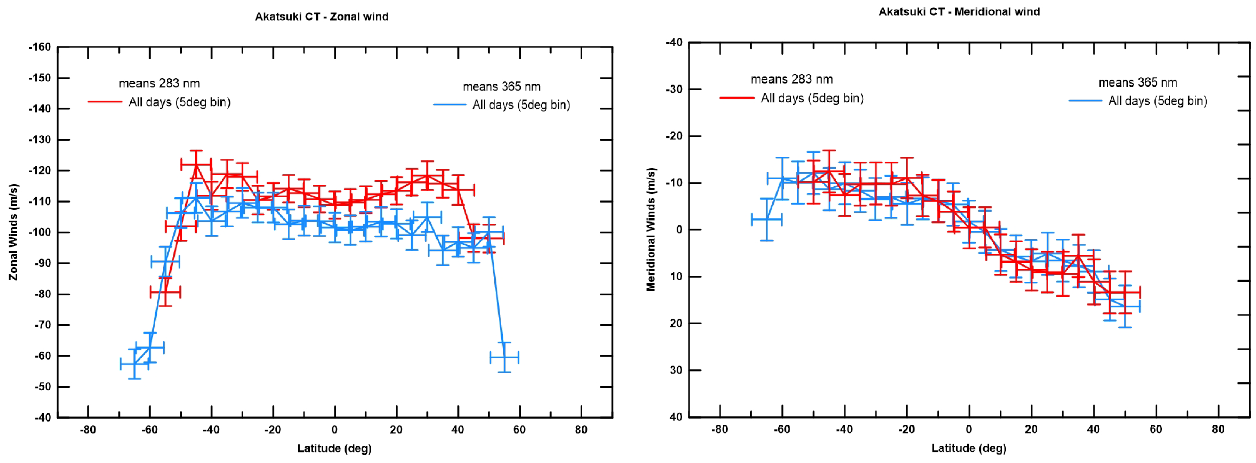
A Comparison of Akatsuki Zonal and Meridional Winds at the 283 nm and 365 nm Filters

As we noted in the Introduction, the Akatsuki/UVI 283 nm filter is sensitive to sulphur dioxide (SO${}_2$) concentration and spatial distribution. Horinouchi et al. [1] wrote that, for cloud-tracked winds, the 283 nm filter sensed higher layers of Venus’ atmosphere than the 365 nm filter for image-based cloud-tracked winds. However, Encrenaz et al. [43] proved that the SO${}_2$ mixing ratio of altitude and spatial distribution was highly variable. The described temporal variability could mean that altitudes sensed with the Akatsuki/UVI 283 nm filter vary from one temporal window dataset to another range of observational dates.

Figure 5 presents a comparison of the latitudinal profiles of zonal (left panel) and meridional (right panel) winds between 26and 31 January 2017. Profiles in red, both zonal and meridional, were retrieved in the context of this work and were related to the cloud-tracked winds obtained by the 283 nm Akatsuki/UVI filter. The profiles in blue colour (zonal and meridional profiles) were obtained in Gonçalves et al. [7] and show the 365 nm filter cloud-tracked winds.

It is clear from Figure 5 that the 283 nm filter zonal wind velocity results were higher than the ones obtained from the 365 nm UVI filter images. In fact, in the midlatitude region (approximately between 50${}^{\circ }$ south and 50${}^{\circ }$ north), the two profiles had an average separation of about 10–15 ± 5 ms${}^{-1}$, even if this difference was more marked in the northern hemisphere. Besides the reported significant difference in the midlatitude region, for latitudes greater than 50${}^{\circ }$, both profiles were nearly coincident in their steep decrease of zonal wind speed.

With respect to the two filters’ (283 and 365 nm) latitudinal meridional wind profiles, the right panel in Figure 5 shows that both profiles were not significantly separated. Even if the 283 nm-related (coloured red in the figure) profile indicated an average velocity higher by a couple of ms${}^{-1}$, we cannot claim as a fact that this wind velocity was really different since it was within the uncertainties connected to the measurement and retrieval process.

4.2. VIRTIS-M VEx Coordinated Cloud-Tracked Results and Comparison with Earlier Similar Works

In February 2014, we conducted a coordinated campaign of Venus’ observations using the Venus Express (VEx) space probe VIRTIS-M instrument observations and almost synchronised ground-based observations with CFHT/ESPaDOnS at Maunakea observatory (Hawaii, USA).

Due to the highly eccentric polar orbit of VEx, it is possible to retrieve cloud-tracked winds using the VIRTIS-M images’ tracers, but only in the southern hemisphere of Venus. Figure 6 shows the mean latitudinal profile zonal wind calculated by cloud-tracking techniques in the visible and ultraviolet domain. For this work, we used wavelength images at 380 nm.

The segment of the latitudinal zonal wind profile, between 30${}^{\circ }$ and 70${}^{\circ }$ latitude south, showed three distinct regions: one nearly uniform zonal wind of ∼100 ms${}^{-1}$ at latitudes below 50${}^{\circ }$, the presence of a midlatitude jet around 50${}^{\circ }$ with an increased wind velocity of the order of 10 ms${}^{-1}$ and a third profile region for higher latitudes than the one previously referenced, where the zonal velocity gradually diminished. To facilitate the visualisation of the zonal wind profile, we also plot in the same figure a profile obtained in an earlier study, also using the same wavelength VEx VIRTIS-M data, from Sánchez-Lavega et al. [19]. The comparison between the two profiles showed that they were highly consistent in the overlapping region.

In Figure 7, we compare the latitudinal mean zonal wind profile obtained (Figure 6) from our space- and ground-based coordinated observing project with VEx VIRTIS-M at 380 nm, with earlier results also using Venus Express/VIRTIS [4,6,19,21] and other space-based zonal wind profiles coming from Akatsuki/UVI at 365 nm [1,7]. Besides some tiny fluctuations, which were expected in the very active and dynamic atmosphere of Venus, although inside the uncertainty level, it was clear from the comparison in the figure that the latitudinal zonal wind profiles were highly consistent among each other.

It is worth highlighting some significant features in these zonal wind latitudinal profiles. These include for example nearly uniform zonal wind velocities in the midlatitude region (between 50${}^{\circ }$ south and 50${}^{\circ }$ north), where the roughly stable zonal wind speed was around 100 ± 5 ms${}^{-1}$; a smooth midlatitude jet (∼50${}^{\circ }$) in both hemispheres—more remarkable in some profiles than others, but peaking at 10 ms${}^{-1}$; a steady and steep decrease of the zonal wind velocity for higher latitudes.

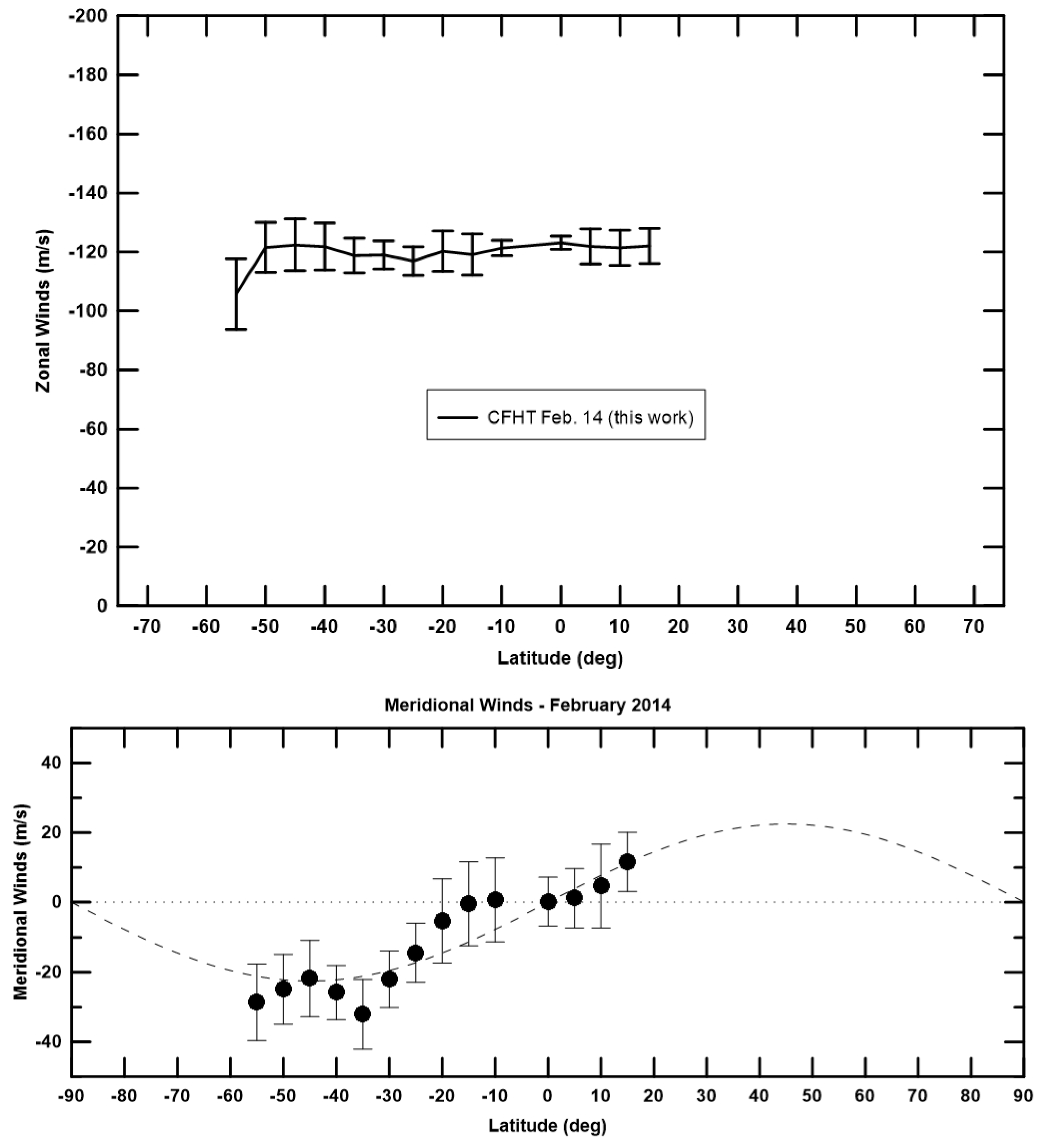
4.3. Wind Results Using Doppler Velocimetry Techniques and CFHT/ESPaDOnS Observations

We applied our Doppler velocimetry technique [4,6,7,11] to the high-resolution spectra that we obtained with the CFHT/ESPaDOnS spectrograph. These observations were part of a coordinated campaign with the space probe Venus Express in February 2014.

The ground-based CFHT/ESPaDOnS Venus observations took the form of examining sequences between 8 and 10 February. Sequences 1–17 were acquired across the dayside hemisphere at latitudinal bands five degrees apart at the latitude/local time points of Table 4 in a 2 h time scale (see Figure 1 and Table 4). On these day of observation, ESPaDOnS had a projected field of view of ∼220 km at the disk centre of Venus.

The zonal wind velocities retrieved at each offset position were weighed means of individual exposures. In general, we note that the Doppler velocities at each one of the data points acquired were self-consistent. The rare cases (less than 5%) where there was a significant deviation (outlier) were discarded. When there was some indication of a poor-quality exposure during the observation run due to passing cirrus clouds or significant drift on ESPaDOnS’s field of view from the chosen offset location, the exposure was repeated immediately. Then, the mean zonal wind velocities retrieved at each position offset were grouped in latitudinal bands, and we performed a weighted average for each one of the sensed latitudinal bands (see Figure 1).

Figure 8 (upper panel) shows the segments of the mean zonal latitudinal profile retrieved from each day of observations (in different colours). As we can see, the several segments of the zonal wind profile related to the three days of observations were consistent among each other, with a slight variability lying inside the uncertainty intervals.

A poleward meridional wind component was determined by selecting the line-of-sight measurements on the half-phase angle meridian (HPA) (see Figure 1), then we applied a dedicated and fine-tuned method [6,7] in order to retrieve the meridional component of the wind along this referenced meridian (see also Section 2.2 herein for details).

In Figure 8 (lower panel), we show the outcome of our dedicated meridional technique applied along the half-phase angle meridian (HPA) for each day of observation (different colours on each represented segment mean each observational day as referred to in the figure legend). Negative velocities in the southern hemisphere in Figure 8 reflect poleward cloud top motion, while positive values in the northern hemisphere also indicate a poleward motion. This is in agreement with a Hadley cell’s upper branch, were the meridional wind flows from the equator region to higher latitudes.

The consolidated latitudinal wind profiles of all observing days are presented in Figure 9. The upper panel shows the mean zonal wind latitudinal profile. From the figure’s analyses, it is clear that the zonal wind is approximately uniform between midlatitudes, with a velocity of around 120 ± 7 ms${}^{-1}$. We can note the presence of a midlatitude jet (at ∼50${}^{\circ }$ in both hemispheres) and a steady decrease of the zonal wind velocity at higher latitudes. Regarding the meridional wind profile (Figure 9, lower panel), we applied the same process to obtain an averaged consolidated profile. The main characteristics of the meridional wind profile consisted of a zero meridional velocity at the equatorial region and a flow from the equator toward the poles in both hemispheres.

4.4. Doppler Wind Results—A Comparison with Similar Previous Studies

In Figure 10, it is possible to compare the results of our earlier Doppler velocimetry studies with the ones we presented here. In the upper panel, we compare several runs using the high-resolution spectrograph ESPaDOnS (CFHT, Hawaii, USA) and also the results based on the UVES (VLT-ESO, Chile). There appeared to be a quite striking high level of coincidence between all the presented latitudinal profiles of zonal winds. Moreover, remember that the observing runs came from temporal windows separated by a considerable amount of time and also that we used two different Doppler velocimetry methods in the data reduction process, one adapted to long-slit spectrographs as in the case of UVES/VLT and one adapted to fibre-fed spectrographs as for the cases of ESPaDOnS/CFHT and HARPS-N/TNG.

Zonal wind profiles showed, in general, a retrograde zonal flow of the wind, nearly homogeneous, of around 120 ± 7 ms${}^{-1}$ and the presence of a midlatitude jet (lower than 10 ms${}^{-1}$) at approximately 50${}^{\circ }$ in both hemispheres with a steep decrease of the zonal wind velocity at higher latitudes.

Figure 10 (lower panel) shows the Doppler velocimetry results for the meridional wind. These latitudinal meridional wind profiles were comprised of several ESPaDOnS/CFHT runs, which included the profile obtained in the context of the present work. The profile obtained from HARPS-N/TNG observations is also shown.

The main characteristics of the latitudinal meridional wind profiles in this figure are: (a) the striking similarities of all profiles, (b) the almost symmetrical behaviour of the meridional flow between the northern and southern hemispheres, (c) the null meridional wind at the equatorial region, (d) the presence of a meridional wind in each hemisphere moving away from the equator and towards the poles, (e) a wind speed maximum at ∼40–45${}^{\circ }$ of 20–25 ± 9 ms${}^{-1}$ and, finally, (f) a decrease of the meridional wind velocity reaching almost zero at about a 60${}^{\circ }$ latitude.

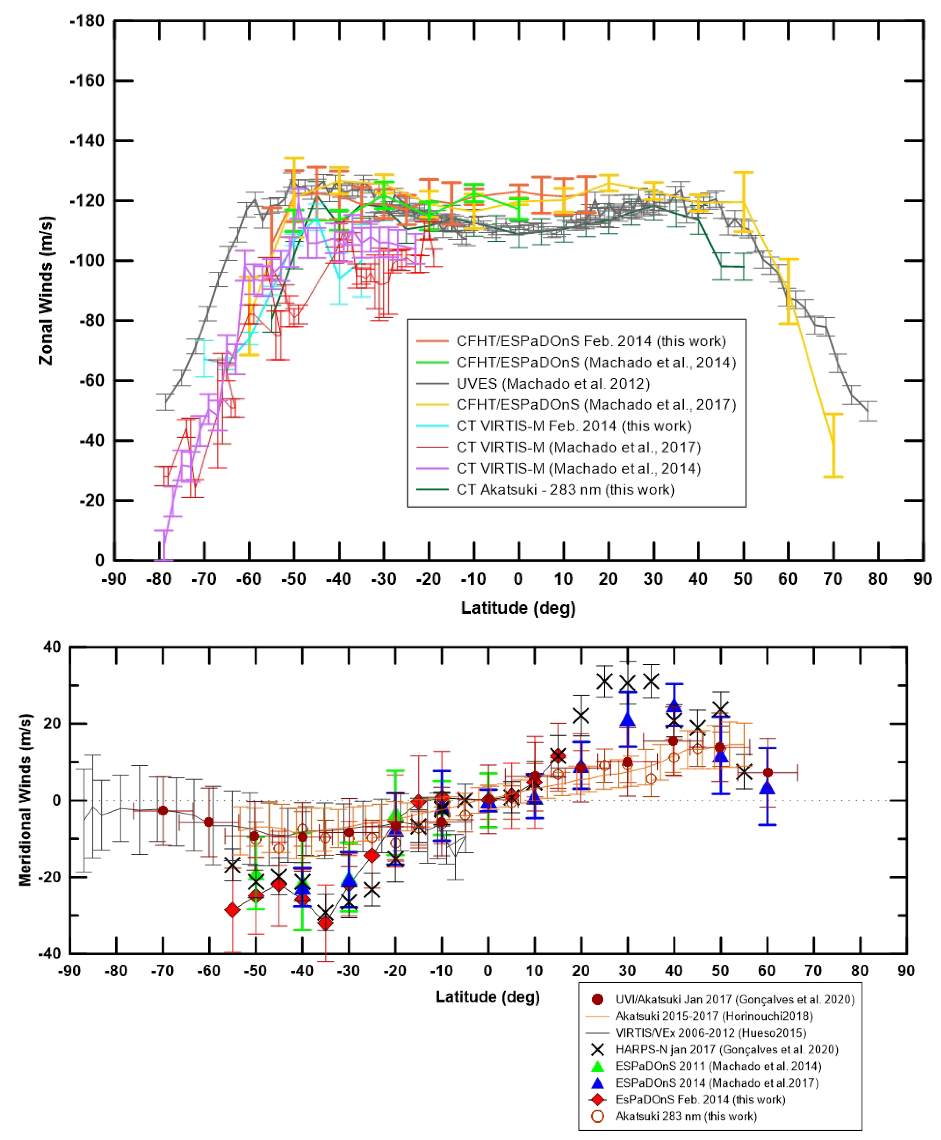
4.5. Doppler and Cloud-Tracked Winds—A Comparison

Figure 10 (upper panel) presents the results from coordinated campaigns of observations (several cases) where we took advantage of synchronous (or almost synchronous) measurements of the atmosphere of Venus made at the cloud top level. We benefited from having access to space-based Venus Express VIRTIS-M (380 nm images) data sets and simultaneous (or almost simultaneous) ground-based observations from CFHT/ESPaDOnS. We also had access to Akatsuki/UVI (365 and 283 nm filter’s images) coordinated with our TNG/HARPS-N observations.

It is possible to make two clear and robust interpretations based on the left panel’s latitudinal zonal wind profiles. On the one hand, space-based cloud-tracked results (VEx/VIRTIS-M (380 nm) and Akatsuki/UVI (365 nm)) were highly consistent with each other (with a midlatitude zonal wind of nearly 100–105 ± 5 ms${}^{-1}$), as well as the Doppler wind-based profiles were highly self-consistent (with a midlatitudes zonal wind of the order of 115–120 ± 7 ms${}^{-1}$).

On the other hand, however, it seems that we could make the solid assumption that the two kinds of zonal wind profiles diverged by an average of 10–15 ms${}^{-1}$ in the midlatitude region. This strongly indicated that the two techniques were, in fact, sensing two slightly different altitude levels in the atmosphere of Venus. Finally, we note that both kinds of zonal wind profiles reached a smooth jet at approximately 50${}^{\circ }$ in both hemispheres, and from there, the zonal wind decreased in a steep and steady way.

As concerns the comparison from cloud-tracked meridional winds using space-based (Figure 10, lower panel) VEx/VIRTIS-M (380 nm) and Akatsuki/UVI (283 and 365 nm), the interpretations that stood out from the figure analysis were twofold: the Doppler profiles were consistent with each other; the cloud-tracked profiles were also consistent with each other them; there was a peak velocity difference of about 10 ms${}^{-1}$ between Doppler profiles and cloud-tracked profiles.

It is clear that all profiles indicated that there was no meridional wind flow at the equatorial region. However, there was an increase of the meridional wind in each hemisphere, flowing poleward from the equator and reaching a peak around a latitude of 40–45${}^{\circ }$, and in all cases, this wind decreased rapidly, reaching zero at around a latitude of 50${}^{\circ }$.

It is surprising that when we compared our Doppler velocimetry results with the ones retrieved using cloud-tracking methods based on Akatsuki/UVI with the 283 nm filter, the respective zonal wind latitudinal profiles were remarkably similar (see Figure 10). Horinouchi et al. [1] already pointed out that the 283 nm filter of the UVI instrument might sense higher altitudes than the other UV filter centred at 365 nm. The 283 nm filter is sensitive to the atmospheric concentration and geographic distribution of SO${}_2$, as we already discussed in the Introduction of the present work. The coincidence is that, at the time of our Akatsuki/UVI dataset temporal window (26–31 January 2017), the atmospheric distribution of SO${}_2$ implied that the level of the altitude layer sensed by the UVI instrument (with the 283 nm filter) was approximately the same as the altitude sensed by our ground-based high-resolution spectrographs. It would seem therefore that the zonal winds retrieved with our Doppler velocimetry technique were most probably sensing a higher altitude layer of the atmosphere of Venus than the 365 (or 380) nm cloud-tracked winds.

4.6. Discussion and a Comparison between Observations and Modelling

In order to address the robust indication provided by the observations that cloud-tracked winds (365–380 nm) and visible Doppler velocimetry winds (and 283 nm cloud-tracking) were, in fact, sensing slightly different altitudes at the cloud tops of Venus’ atmosphere, we compared the retrieved data in the context of the present work with previous reference results and with results from other coordinated observations in the framework of the present atmospheric dynamical study.

The modelling predicted profiles of zonal wind used in the present comparison (see Figure 11, Figure 12 and Figure 13) came from improved versions of the IPSL Venus General Circulation Model (IPSL-VGCM) [24,25] and the AFES-Venus GCM [41,42]. The predicted latitudinal profiles of zonal wind used in these figures, for the purposes of comparison, were extracted from the IPSL-VGCM and AFES-Venus model outputs at different pressure levels, from 4 kPa to 7 kPa (corresponding to different altitudes in the atmosphere of Venus), to represent the mean cloud top altitudes (∼68–74 km) as observed [14,46], and averaged for daytime local times (10 h–17 h) to be consistent with the observations.

Figure 11 considers the cloud-tracked zonal wind and compares the results obtained from VEx VIRTIS-M (380 nm) observations in the context of the coordinated observations presented in this work, with other reference profiles using similar methods and also using the same instruments [6,19,21], as well as with the relevant results of zonal wind that were based on Akatsuki/UVI (365 nm filter) observations [1,7]. We selected the best fit altitude profiles from the IPSL-VGCM [24,25] and the AFES-Venus GCM [41,42] and performed an average from all the predicted latitudinal zonal wind profiles covering the dayside local time range covered by the observations. The final average model results are presented in Figure 11, as a band coloured in light blue (IPSL-VGCM) and in light green for the AFES-Venus model plot (Figure 11).

From our interpretation indicated in Figure 11, it is clear that cloud-tracked (VEx VIRTIS-M (380 nm) and Akatsuki/UVI (365 nm)) latitudinal zonal wind profiles were highly consistent. Zonal wind modelling profiles (IPSL-VGCM) strongly suggested that the atmospheric altitudes that best matched with referenced observational results were at an altitude of approximately 68 km. Naturally, the referred altitude is a first guess and will need further confirmation. Midlatitude zonal wind observational results pointed to a roughly uniform velocity of around 100 ± 5 ms${}^{-1}$. However, one can note that the modelling profiles were wider in latitude than the whole set of self-consistent observational profiles. The magnitude of the zonal wind velocities tended to decrease rapidly at nearly 50–55${}^{\circ }$ in both hemispheres, while the IPSL-VGCM profiles extended to higher latitudes, and zonal velocity diminished at a less steep and slower rate. Regarding the AFES-Venus model’s prediction, it was clear that, besides the high consistency with observational results in the midlatitudes region, the midlatitudes jet was more pronounced in the model profile.

In Figure 12, we compare the latitudinal profiles of meridional wind flow obtained using our Doppler velocimetry method and based on observations made with the high-resolution spectrograph ESPaDOnS at CFHT, with meridional modelling predictions from Sugimoto et al. [41], Takagi et al. [42], Takagi and Matsuda [47] and from IPSL-VGCM [24,25]. The meridional wind profiles retrieved from observations and presented here were an average of all the days’ observations for each run (from three to seven days in the profiles shown in this figure). The prediction profiles best matched with the observational ones were from a five-day average at an altitude of 70 km (AFES-Venus) and between 68 and 72 km for IPSL-VGCM.

The main highlights of the analyses shown in Figure 12 are as follows: meridional flow deduced from ground-based observations were self-consistent; there was a high level of agreement between the AFES-Venus model-predicted latitudinal profile of the meridional wind velocity and observations; near the equator, the meridional flow was almost absent; there was a poleward meridional flow for each hemisphere, which after reaching a peak of about 20 ± 5 ms${}^{-1}$ at approximately 45${}^{\circ }$ latitude, started to decrease until it became almost absent at about 60${}^{\circ }$. The described behaviour of the observational-based profiles was consistent with the AFES-Venus model-predicted profile, while the predicted profiles from the IPSL-VGCM extended the meridional flow to the polar region, which diverged from all observational profiles’ results, which tended to decrease the meridional wind velocity at nearly 45${}^{\circ }$ of latitude for each hemisphere.

Figure 13 presents the latitudinal zonal wind velocity profiles based on ground-based observations (using VLT/UVES [11] and CFHT/ESPaDOnS (Machado et al. [4], Machado et al. [6] and the present work using high-resolution spectra and Doppler velocimetry methods). Shown also is the zonal wind profile retrieved from space-based observations with the Akatsuki/UVI instrument and its 283 nm filter (this work).

From the Venus atmosphere IPSL-VGCM [24,25] and AFES-Venus [41,42], latitudinal profiles of zonal wind at several altitudes were extracted, which corresponded to different pressure levels in the model. The predicted profiles that matched the observational-based zonal wind profiles best were averaged in local time for all the dayside meridian range model profiles covered by the observations. Finally, the mean zonal wind profiles predicted by the models are also plotted, in yellow (AFES-Venus) and in a band coloured in light red (IPSL-VGCM), in Figure 13 for comparison purposes.

From the analyses shown in Figure 13, it is clear that the zonal wind latitudinal profiles indicated by Doppler techniques and by cloud tracking (283 nm) were consistent. The best fit zonal wind modelling profiles (IPSL-VGCM and AFES-Venus) indicated that most probably, the altitude sensed with ground-based visible Doppler techniques and space-based cloud tracking (283 nm) was approximately 72 km. Zonal wind velocity in the midlatitude region was about 110–120 ± 7 ms${}^{-1}$ and dropped in a steady, but steep way for latitudes higher than 50–55${}^{\circ }$ in both hemispheres. We can note that in the predicted profiles, the zonal wind velocity from AFES-Venus was highly consistent with the profiles based on observations. The same was valid for the profiles predicted by IPSL-VGCM between midlatitudes; however, in this case, the predicted zonal wind velocity profiles decreased at higher latitudes than in the case of the cloud-tracking (283 nm) and Doppler-based latitudinal zonal wind profiles.

5. Conclusions

New results of zonal and meridional winds in both hemisphere of Venus were presented in this study from ground- and space-based coordinated observations, using two complementary techniques: the Doppler velocimetry (DV) and cloud tracking (CT). We list the main conclusions here.

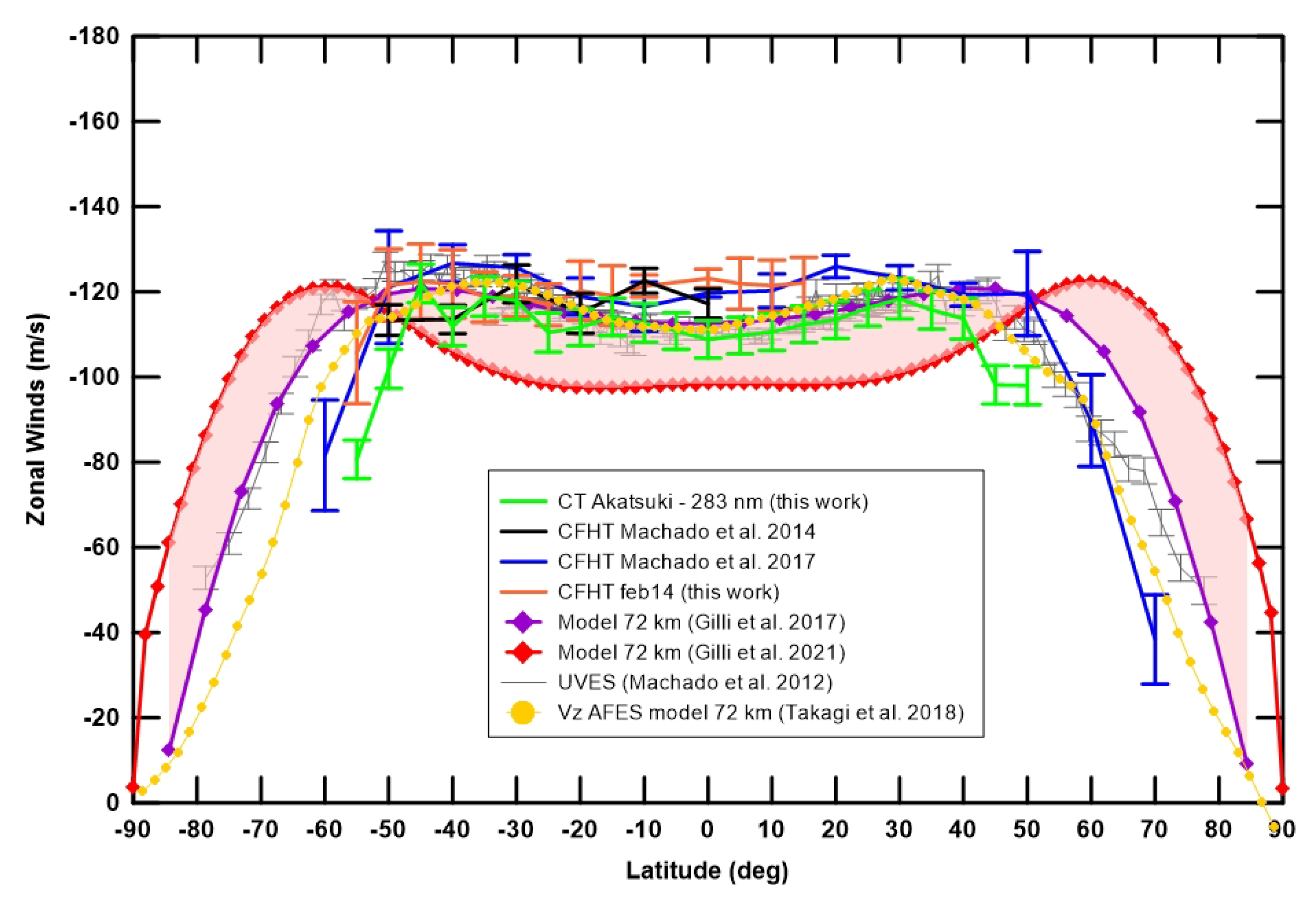
• CT zonal winds from Akatsuki UVI observations (283 nm filter) of 26–31 January 2017 presented in this work were roughly consistent among all days of observations in this dataset. However, they were on average higher (of the order of 10–15 ± 5 ms${}^{-1}$) than the ones retrieved with the 385 nm filter and related to the same period [7]. Related latitudinal profiles showed an almost uniform velocity (115–120 ± 5 ms${}^{-1}$) in the midlatitudes region (50${}^{\circ }$N–50${}^{\circ }$S), where it peaked at nearly 125 ± 5 ms${}^{-1}$, decreasing in a steep and steady way for higher latitudes. Nevertheless, a general daily variability of about 5–10 ± 5 ms${}^{-1}$, both spatial and temporal, affected the zonal wind field. The asymmetry between hemispheres noted in the 365 nm image-based CT winds [7] was not evident in the 283 nm-related results of the present work.
• We measured near-zero meridional wind velocity in the equatorial region, a poleward meridional flow peaking (∼20 ± 5 ms${}^{-1}$) at about 45${}^{\circ }$ in latitude and, from there, decreasing steeply in magnitude. The described behaviour of the meridional flow was compatible with the existence of a Hadley cell-type in each hemisphere of Venus [6]. The daily wind variability was in general of the order of 5 ms${}^{-1}$. However, in one of the days of observations (26 February), it reached approximately 8 ms${}^{-1}$. We note an asymmetry between hemispheres where the meridional flow increased by some 5 ms${}^{-1}$ in the north compared to the corresponding southern latitudes.
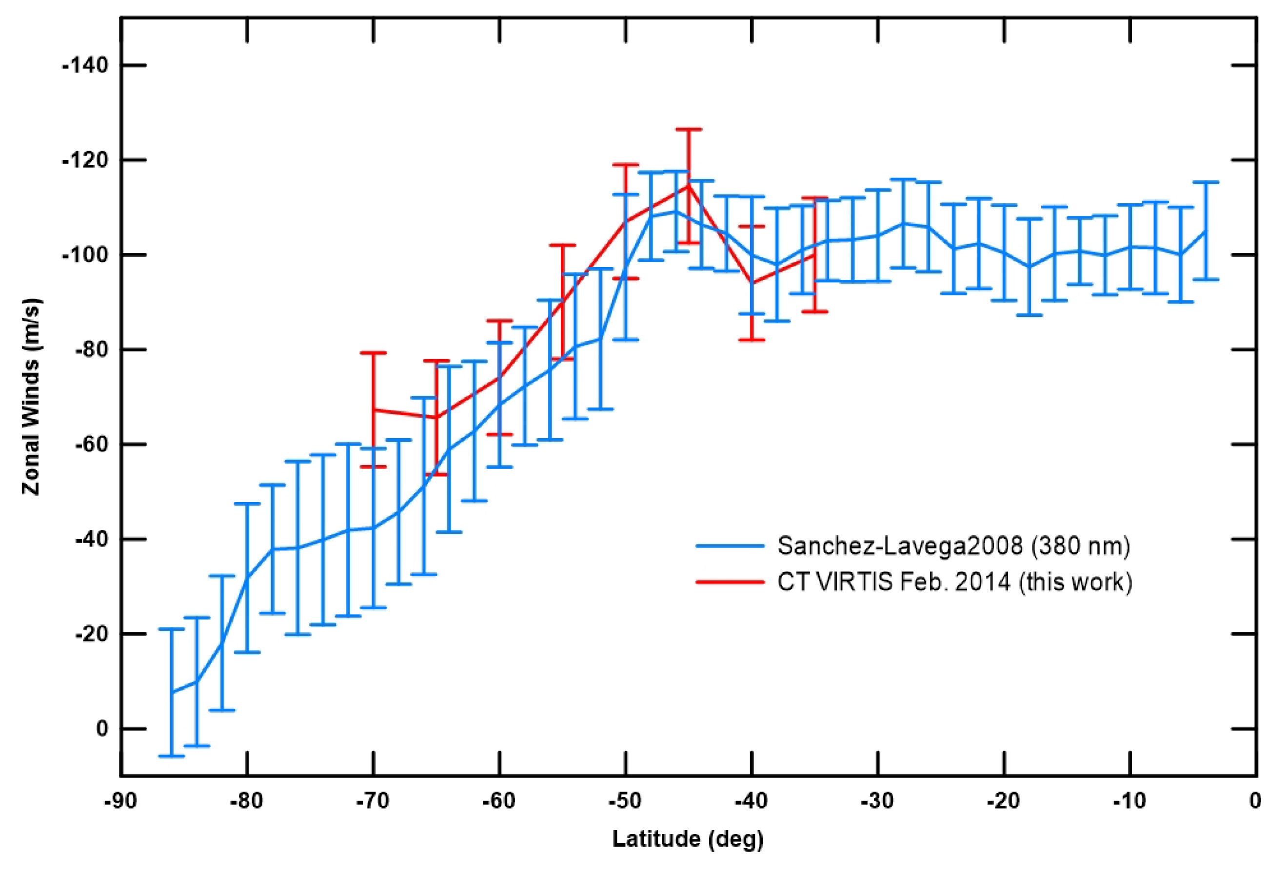
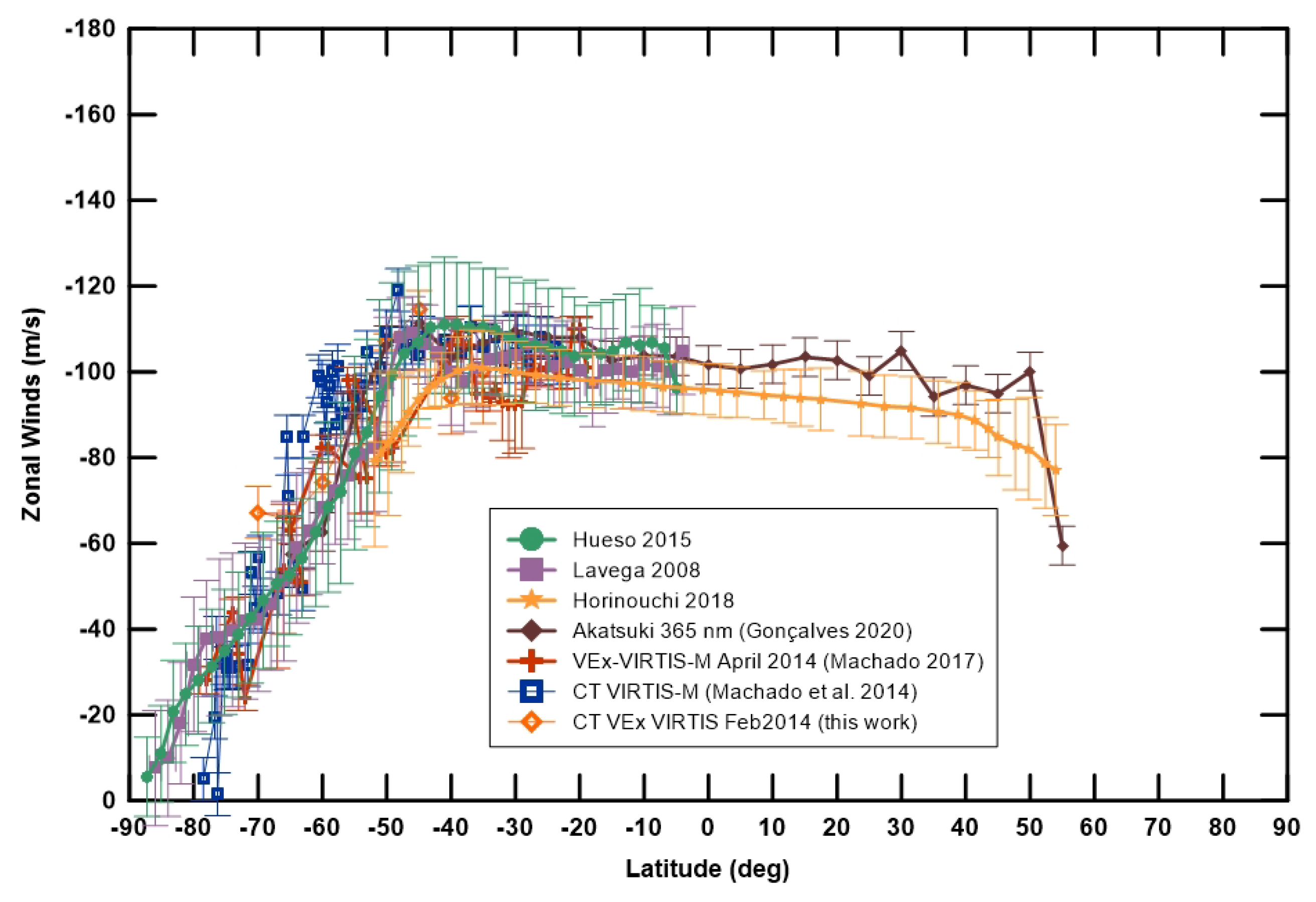
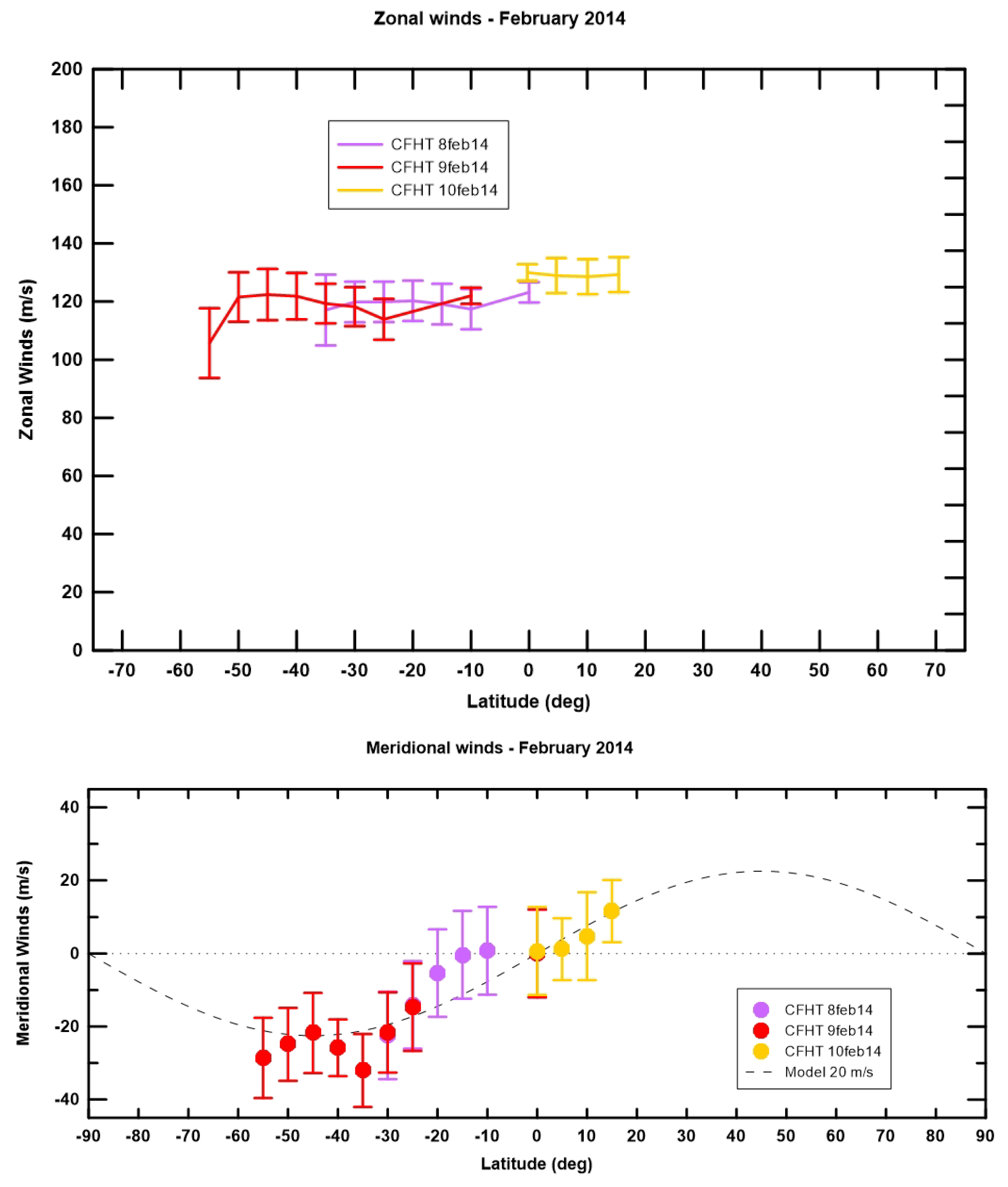
• The results from our coordinated observing campaign from space-based VEx VIRTIS-M (380 nm) CT winds (February 2014) indicated that they were comparable with the Akatsuki/UVI 365 nm filter and with other VEx/VIRTIS ultraviolet images centred at 380 nm [19,20,21] or other Akatsuki/UVI (365 nm) results [1,7]. With respect to our observations with CFHT/ESPaDOnS and their related Doppler wind retrieved from high-resolution spectra (R ∼ 80,000), both zonal and meridional wind components were consistent with previous results [4,6,11] and with the 283 nm Akatsuki UVI-based CT results. However, Doppler winds were about 10–15 ± 5 ms${}^{-1}$ larger than the VIRTIS-M (380 nm) observation-retrieved winds. Horinouchi et al. [1] suggested that the 283 nm images probably reflected cloud features at a higher altitude than the 365 nm (and 380 nm) images. While the UVI 365 nm-centred filter tracks cloud features produced by an unknown UV absorber, the 283 nm filter was designed to match and probe a SO${}_2$ absorption band. However, the SO${}_2$ vertical distribution and the variability of concentration along local time and latitude are still not fully constrained [22,43].
• Our results suggested that the CT technique based on cloud images contrasted by the unknown UV absorber (VEx/VIRTIS at 380 nm and Akatsuki/UVI at 365 nm) and our visible DV technique, apart from probing different features and phenomena at the clouds, might also be probing different altitudes of Venus’ atmosphere. The DV technique constitutes a complementary way of probing the cloud tops of Venus and a unique approach from the ground, given that this method directly measures the motion of the aerosol particles and the retrieved wind velocities, which are instantaneous measurements. It should also be noted that the fluctuations in velocity measured with CT involve eddy and wave motions. Instead, the cloud top altitude where the DV winds are measured varies with latitude, decreasing especially near the poles [14,38]. Peralta et al. [5] also estimated the vertical profile of zonal winds during the second Venus flyby of NASA’s Messenger spacecraft, and their results suggested, on the dayside, the altitude at which the zonal wind peaks seem to vary over time.
• Since the solar back-scattered light dispersed from the atmosphere of Venus is the result of a bolometric integration of all the back-scattered solar radiation towards the line-of-sight of ground-based observers, the average radiation that arrives at the instrument’s detector could in fact be coming from a couple of kilometres higher than the cloud tops. However, tracked UV features may be positioned at a variety of altitudes within the upper cloud top layers. Therefore, the unknown nature and temporal distribution of the structures of the dark cloud features along the cloud width thickness, due to the UV absorber, may lead to an uncertainty in the altitude of the cloud features of several kilometres. Obviously, this is just a tentative explanation, based on observational evidence, for the fact that DV and CT (365 nm or 380 nm) are sensing slightly different altitudes in the atmosphere of Venus. For full clarification of this issue, we intend to perform dedicated observations in the near future and take advantage of a radiative transfer tool to address the reported difference in detail.
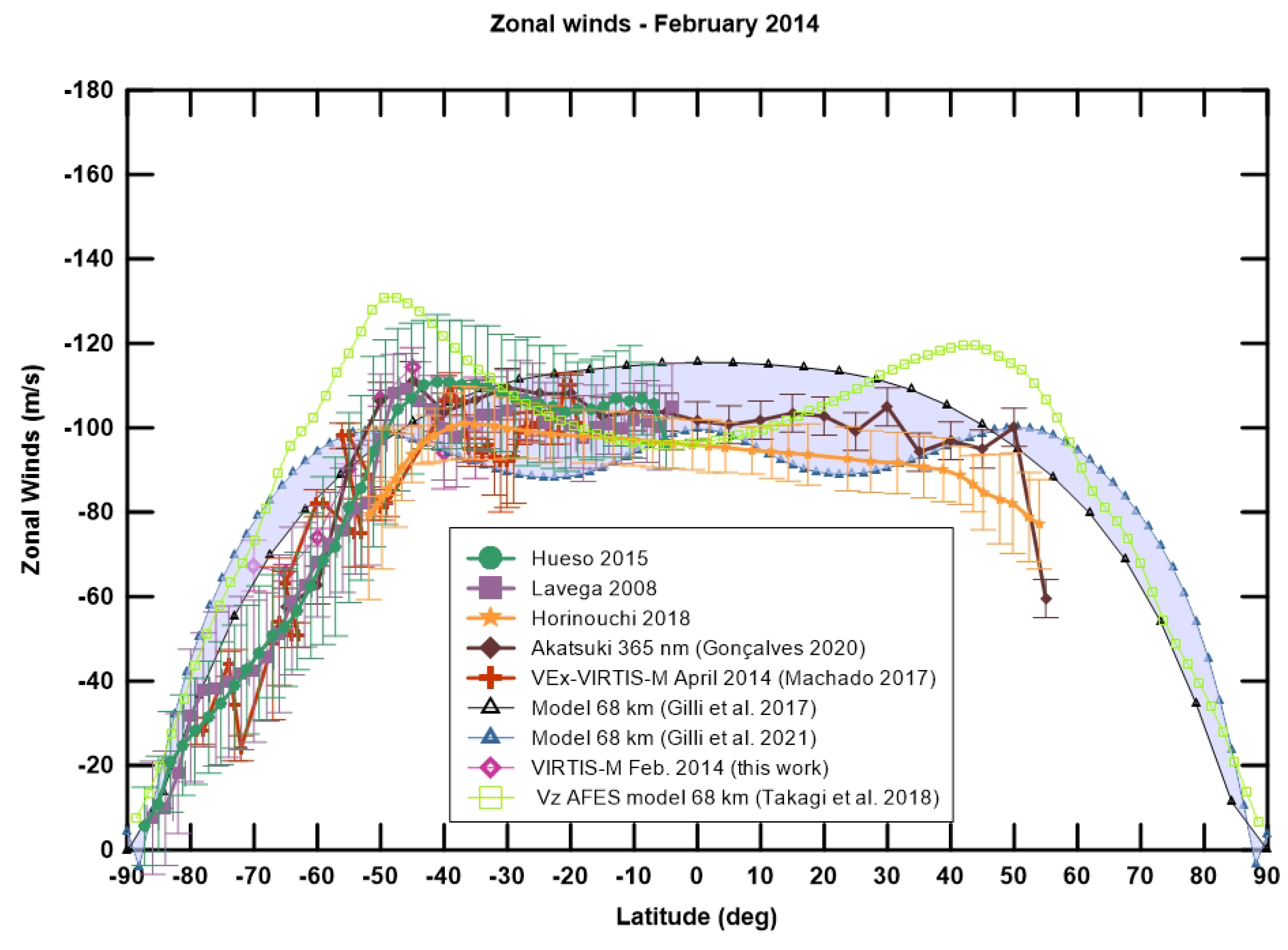
• Following the evidence of a systematic observational difference in altitudes probed by DV and CT winds, both from Akatsuki/UVI filters and the 380 nm VEx/VIRTIS-M images, we also compared wind measurements with Venus’ GCM predictions of zonal wind velocity at approximately the cloud top. Although a good agreement was found between the observational-based profiles and the predicted ones from IPSL-VGCM [24,25], the latter are overall wider in latitude (about a 10–15${}^{\circ }$ extended latitude range between midlatitudes jets location). It may be linked to the uncertainties of the observational properties of the cloud structure assumed in the IPSL-VGCM model. Furthermore, notice that the altitude values in the model were approximated and the model cannot appreciate a variation of less than 2 km, because of its vertical resolution. With respect to AFES-Venus’ [41,42] best fit predicted profile at an altitude of 68 ± 2 km, Figure 11 clearly shows good agreement with observations between midlatitudes, but with more pronounced midlatitude jets predicted by the model.
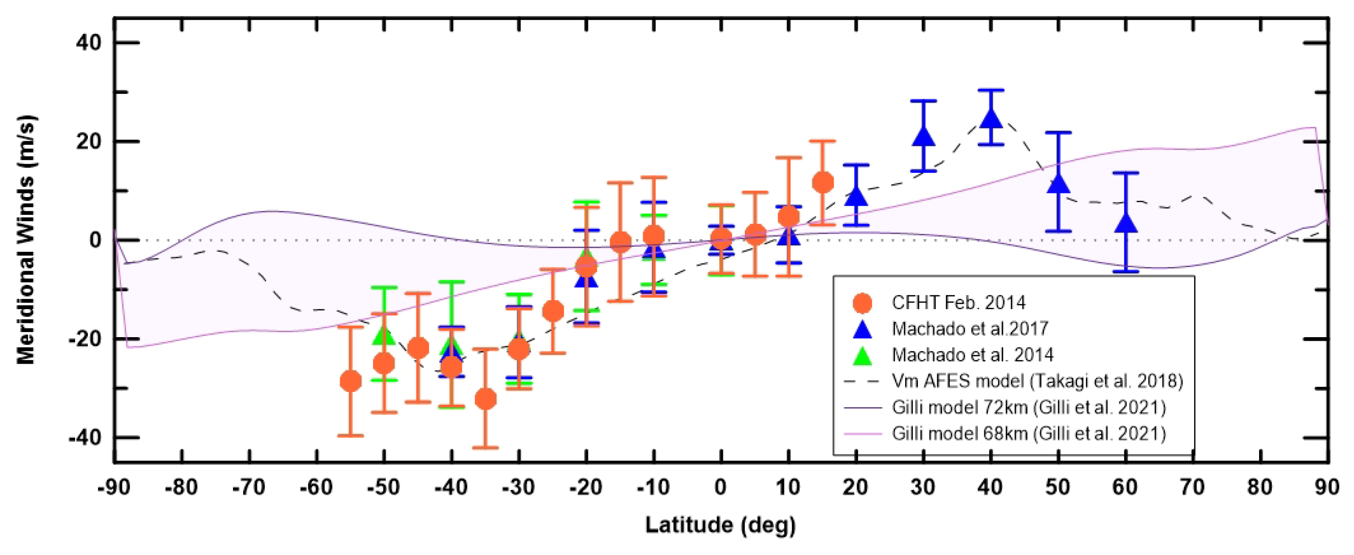
• For the meridional wind flow, we compared our results with the AFES-Venus GCM and IPSL-VGCM where the matching of the plots showed a high level of consistency between our measurements and the predicted profiles (see Figure 12). Recently, Takagi et al. [42] suggested that the Hadley-type circulation might be confined to latitudes equatorward to a maximum of 70${}^{\circ }$, which is in good agreement with our observed results. The comparison with IPSL-VGCM predictions showed that the meridional flow modelled extended to the poles, which was not seen in any observational profile (CT or DV). In general, all observational-based profiles dropped the meridional velocities at the midlatitude region (∼50–65${}^{\circ }$ latitude).

All in all, this work shows:

(1)

Additional confirmation of the coherence and complementarity in the results provided by the DV and CT techniques on both the spatial and temporal time scales of the two methods.

(2)

An estimation of an upper-branch meridional component of the wind using the Doppler velocimetry technique and cloud-tracked winds as well (283, 365 and 380 nm), with evidence of a symmetrical, poleward meridional Hadley-type flow in both hemispheres.

(3)

Even though the results presented in this paper do not constitute an unambiguous proof by themselves, they provide evidence that the altitude of zonal wind probed by the DV technique is highly consistent with both the UVI 283 nm filter and the model predictions at about 72 km of the IPSL-VGCM [24,25] and AFES-Venus [41,42].

(4)

The altitude of the CT results, from both VEx/VIRTIS-M (Machado et al. [6], Hueso et al. [21] and this work) and Akatsuki/UVI 385 nm filter [1,7], was highly consistent with Venus’ LMD GCM [24,25] and AFES-Venus [41,42] predictions at altitudes around 68 km. Therefore, a difference in altitude of up to 4 ± 2 km could be enough to explain the difference in the referenced measurements of wind velocities from DV and CT. Moreover, from now on, we can rely on a new tool to study and constrain the vertical wind shear at the level of the top of the clouds in Venus’ atmosphere.

References

1. Horinouchi, T.; Kouyama, T.; Joo Lee, Y.; Murakami, S.; Ogohara, K.; Takagi, M.; Imamura, T.; Nakajima, K.; Peralta, J.; Yamazaki, A. Mean winds at the cloud top of Venus obtained from two wavelength UV imaging by Akatsuki, Earth. Plan. Space 2018, 70. [Google Scholar]
2. Drossart, P.; Piccioni, G.; Gérard, J.C.; Lopez-Valverde, M.A.; Sanchez-Lavega, A.; Zasova, L.; Hueso, R.; Taylor, F.W.; Bézard, B.; Adriani, A.; et al. A dynamic upper atmosphere of Venus as revealed by VIRTIS on Venus Express. Nature 2007, 450, 641–645. [Google Scholar] [CrossRef] [PubMed]
3. Titov, D.M.; Titov, F.W.; Taylor, H.; Svedhem, N.I.; Ignatiev, W.J.; Markiewicz, G.; Piccioni, P.D. Atmospheric structure and dynamics as the cause of ultravioletmarkings in the clouds of Venus. Nature 2008, 456, 620–623. [Google Scholar] [CrossRef] [PubMed]
4. Machado, P.; Widemann, T.; Luz, D.; Peralta, J. Wind circulation regimes at Venus’ cloud tops: Ground-based Doppler velocimetry using CFHT/ESPaDOnS and comparison with simultaneous cloud tracking measurements using VEx/VIRTIS in February 2011. Icarus 2014, 243, 249–263. [Google Scholar] [CrossRef]
5. Peralta, J.; Lee, Y.J.; Hueso, R.; Clancy, R.T.; Sandor, B.; Sànchez-Lavega, A.; Imamura, T.; Omino, M.; Machado, P.; Lellouch, E.; et al. The Winds of Venus during the Messenger’s Flyby. 2017. Available online: https://agupubs.onlinelibrary.wiley.com/doi/full/10.1002/2017GL072900 (accessed on 30 March 2021).
6. Machado, P.; Widemann, T.; Peralta, J.; Gonçalves, R.; Donati, J.; Luz, D. Venus cloud-tracked and doppler velocimetry winds from CFHT/ESPaDOnS and Venus Express/VIRTIS in April 2014. Icarus 2017, 285, 8–26. [Google Scholar] [CrossRef]
7. Gonçalves, R.; Machado, P.; Widemann, T.; Peralta, J.; Watanabe, S.; Yamazaki, A.; Silva, J. Venus’ cloud top wind study: Coordinated Akatsuki/UVI with cloud tracking and TNG/HARPS-N with Doppler velocimetry observations. Icarus 2020, 335, 113418. [Google Scholar] [CrossRef]
8. Nakamura, M.; Imamura, T.; Ishii, N.; Abe, T.; Kawakatsu, Y.; Hirose, C.; Kamata, Y. AKATSUKI returns to Venus, Earth. Planet. Space 2016, 68, 201668. [Google Scholar] [CrossRef] [Green Version]
9. Yamazaki, A.; Yamada, M.; Joo Lee, Y.; Watanabe, S.; Horinouchi, T.; Murakami, S.; Kouyama, T.; Ogohara, K.; Imamura, T.; Sato, T.; et al. Ultraviolet imager on venus orbiter Akatsuki and its initial results. Earth Planet. Space 2018, 70, 23. [Google Scholar] [CrossRef] [Green Version]
10. Widemann, T.; Lellouch, E.; Donati, J.F. Venus Doppler winds at cloud tops observed with ESPaDOnS at CFHT. Planet. Space Sci. 2008, 56, 1320–1334. [Google Scholar] [CrossRef]
11. Machado, P.; Luz, D.; Widemann, T.; Lellouch, E.; Witasse, O. Characterizing the atmospheric dynamics of Venus from ground-based Doppler velocimetry. Icarus 2012, 221, 248–261. [Google Scholar] [CrossRef]
12. Hansen, J.; Hovenier, J. Interpretation of the polarization of Venus. J. Atmos. Sci. 1974, 31, 1137–1160. [Google Scholar] [CrossRef]
13. Kawabata, K.; Coffeen, D.; Hansen, J.; Lane, W.; Sato, M.; Travis, L. Cloud and haze properties from Pioneer Venus polarimetry. J. Geophys. Res. 1980, 85, 8129–8140. [Google Scholar] [CrossRef]
14. Ignatiev, N.I.; Titov, D.V.; Piccioni, G.; Drossart, P.; Markiewicz, W.J.; Cottini, V.; Manoel, N. Altimetry of the Venus cloud tops from the Venus Express observations. J. Geophys. Res. 2009, 114, E00B43. [Google Scholar] [CrossRef]
15. Fedorova, A.; Marcq, E.; Luginin, M.; Korablev, O.; Bertaux, J.L.; Montmessin, F. Variations of water vapor and cloud top altitude in the Venus’ mesosphere from SPICAV/VEx observations. Icarus 2016, 275, 143–162. [Google Scholar] [CrossRef]
16. Moissl, R.; Khatuntsev, I.; Limaye, S.S.; Titov, D.V.; Markiewicz, W.J.; Ignatiev, N.I.; Hviid, S.F. Venus cloud top winds from tracking UV features in Venus Monitoring Camera. J. Geophys. Res. 2009, 114, E00B31. [Google Scholar] [CrossRef] [Green Version]
17. Lee, Y.J.; Titov, D.V.; Tellmann, S.; Piccialli, A.; Ignatiev, N.; Pätzold, M.; Häusler, B.; Piccioni, G.; Drossart, P. Vertical structure of the Venus cloud top from the VeRa and VIRTIS observations onboard Venus Express. Icarus 2012, 217, 599–609. [Google Scholar] [CrossRef]
18. Esposito, L.W.; Bertaux, J.F.; Krasnopolsky, V.A.; Moroz, V.I.; Zasova, L.V. Chemistry of Lower Atmosphere and Clouds. In Venus II: Geology, Geophysics, Atmosphere, and SolarWind Environment, 1st ed.; Bougher, L.W., Bertaux, J.F., Krasnopolsky, V.A., Moroz, V.I., Zasova, L.V., Eds.; University of Arizona Press: Arizona, United States, 1997; Volume 1. [Google Scholar]
19. Sánchez-Lavega, A.; Hueso, R.; Piccioni, G.; Drossart, P.; Peralta, J.; Perez-Hoyos, S.; Lebonnois, S. Variable winds on Venus mapped in three dimensions. Geophys. Res. Lett. 2008, 35. [Google Scholar] [CrossRef] [Green Version]
20. Hueso, R.; Peralta, J.; Sanchez-Lavega, A. Assessing the long-term variability of Venus winds at cloud level from VIRTIS-Venus Express. Icarus 2012, 217, 585–598. [Google Scholar] [CrossRef]
21. Hueso, R.; Peralta, J.; Garate-Lopez, I.; Bados, T.V.; Sanchez-Lavega, A. Six years of Venus winds at the upper cloud level from UV, viqible and near infrared observations from VIRTIS on Venus Express. Planet. Space Sci. 2015, 113–114, 78–99. [Google Scholar] [CrossRef]
22. Encrenaz, T.; Greathouse, T.K.; Marcq, E.; Sagawa, H.; Widemann, T.; Bézard, B.; Fouchet, T.; Lefevre, F. HDO and SO2 thermal mapping on Venus—IV. Statistical analysis of the SO2 plumes. Astron. Astrophys. 2019, 623, A70. [Google Scholar] [CrossRef] [Green Version]
23. Peralta, J.; Muto, K.; Hueso, R.; Horinouchi, T.; Sánchez-Lavega, A.; Murakami, S.Y.; Luz, D. Nightside Winds at the Lower Clouds of Venus with Akatsuki/IR2: Longitudinal, Local Time, and Decadal Variations from Comparison with Previous Measurements. Astrophys. J. Suppl. Ser. 2018, 239, 29. [Google Scholar] [CrossRef] [Green Version]
24. Gilli, G.; Lebonnois, S.; González-Galindo, F.; López-Valverde, M.A.; Stolzenbach, A.; Lefèvre, F.; Chaufray, J.Y.; Lott, F. Thermal structure of the upper atmosphere of Venus simulated by a ground-to-thermosphere GCM. Icarus 2017, 281, 55–72. [Google Scholar] [CrossRef]
25. Gilli, G.; Navarro, T.; Lebonnois, S.; Trucmuche, A. Venus’ upper atmosphere revealed by a GCM: II. Validation with temperature and densities measurements. Icarus 2021. under revision. [Google Scholar] [CrossRef]
26. Bevington, P.R.; Robinson, D.K. Data Reduction and Error Analysis for the Physical Sciences, 2nd ed.; McGraw-Hill: New York, NY, USA, 1992. [Google Scholar]
27. Donati, J.F.; Semel, M.; Carter, B.D.; Rees, D.E.; Cameron, A.C. Spectropolarimetric observations of active stars. Mon. Not. R. Astron. Soc. 1997, 291, 658–682. [Google Scholar] [CrossRef]
28. Young, A. Is the Four-Day “Rotation”of Venus Illusory? Icarus 1975, 24, 1–10. [Google Scholar] [CrossRef]
29. Gaulme, P.; Schmider, F.-X.; Gonçalves, I. Measuring planetary atmospheric dynamics with Doppler spectroscopy. Astron. Astrophys. 2018, 617, A41. [Google Scholar] [CrossRef] [Green Version]
30. Civeit, T.; Appourchaux, T.; Lebreton, J.-P.; Luz, D.; Courtin, R.; Neiner, C.; Witasse, O.; Gautier, D. On measuring planetary winds using high-resolution spectroscopy in visible wavelengths. Astron. Astrophys. 2005, 431, 1157–1166. [Google Scholar] [CrossRef]
31. Luz, D. UVES measurements of Saturn’s winds with the Absolute Accelerometry technique. Geophys. Res. Abstr. 2005, 7. [Google Scholar]
32. Luz, D.; Civeit, T.; Courtin, R.; Lebreton, J.P.; Gautier, D.; Witasse, O.; Kostiuk, T. Characterization of zonal winds in the stratosphere of Titan with UVES: 2. Observations coordinated with the Huygens Probe entry. J. Geophys. Res. 2006, 111, E08S90. [Google Scholar] [CrossRef] [Green Version]
33. Widemann, T.; Lellouch, E.; Campargue, A. New wind measurements in Venus lower mesosphere from visible spectroscopy. Planet. Space Sci. 2007, 55, 1741–1756. [Google Scholar] [CrossRef]
34. Young, A.; Schorn, R.; Young, L.; Crisp, D. Spectroscopic observations of winds on Venus, I-technique and data reduction. Icarus 1979, 38, 435–450. [Google Scholar] [CrossRef]
35. Lebonnois, S.; Sugimoto, N.; Gilli, G. Wave analysis in the atmosphere of Venus below 100-km altitude, simulated by the LMD Venus GCM. Icarus 2016, 378, 38–51. [Google Scholar] [CrossRef] [Green Version]
36. Garate-Lopez, I.; Lebonnois, S. Latitudinal variation of clouds’ structure responsible for Venus’ cold collar. Icarus 2018, 314, 1–11. [Google Scholar] [CrossRef] [Green Version]
37. Navarro, T.; Schubert, G.; Lebonnois, S. Atmospheric mountain wave generation on Venus and its influence on the solid planet’s rotation rate. Nat. Geosci. 2018, 11, 487–491. [Google Scholar] [CrossRef]
38. Titov, D.; Markiewicz, W.; Ignatiev, N.; Li, S.; Limaye, S.; Sanchez-Lavega, A.; Hesemann, J.; Almeida, M.; Roatsch, T.; Matz, T.; et al. Morphology of the cloud tops as observed by the venus express monitoring camera. Icarus 2012, 217, 682–701. [Google Scholar] [CrossRef]
39. Schubert, G. General circulation and the dynamical state of the Venus atmosphere. Venus 1983, 681–765. [Google Scholar]
40. Navarro, T.; Gilli, G.; Schubert, G.; Lebonnois, S.; Lefèvre, F.; Quirino, D. Venus’ upper atmosphere revealed by a GCM: I. Structure and variability of the circulation. Icarus 2021. under revision. [Google Scholar] [CrossRef]
41. Sugimoto, N.; Takagi, M.; Matsuda, Y. Waves in a Venus general circulation model. Geophys. Res. Lett. 2014, 41, 7461–7467. [Google Scholar] [CrossRef]
42. Takagi, M.; Sugimoto, N.; Ando, H.; Matsuda, Y. Three-dimensional structures of thermal tides simulated by a Venus GCM. J. Geophys. Res. Planet. 2018, 123. [Google Scholar] [CrossRef]
43. Encrenaz, T.; Greathouse, T.K.; Roe, H.; Richter, M.; Lacy, J.; Bézard, B.; Fouchet, T.; Widemann, T. HDO and SO2 thermal mapping on Venus: Evidence for strong SO2 variability. Astron. Astrophys. 2012, 543, A153. [Google Scholar] [CrossRef] [Green Version]
44. Cardesín, A. Study and Implementation of the End-to-End Data Pipeline for the VIRTIS Imaging Spectrometer on Board Venus Express: From Science Operation Planning to Data Archiving and Higher Level Processing. Ph.D. Thesis, Centro Interdipartimentale di Studi e Attività Spaziali (CISAS), Universita degli Studi di Padova, Padova, Italy, January 2010. [Google Scholar]
45. Kouyama, T.; Imamura, T.; Nakamura, M.; Satoh, T.; Futaana, Y. Long-term variation in the cloud-tracked zonal velocities at the cloud top of Venus deduced from Venus Express VMC images. J. Geophys. Res. Planet. 2013, 118, 37–46. [Google Scholar] [CrossRef]
46. Haus, R.; Kappel, D.; Arnold, G. Radiative heating and cooling in the middle and lower atmosphere of Venus and responses to atmospheric and spectroscopic parameter variations. Planet. Space Sci. 2015, 117, 262–294. [Google Scholar] [CrossRef] [Green Version]
47. Takagi, M.; Matsuda, Y. Effects of thermal tides on the Venus atmospheric superrotation. J. Geophys. Res. 2007, 112, D09112. [Google Scholar] [CrossRef]
Figure 1. Observations’ strategy with the Canada-France-Hawaii Telescope (CFHT) and the high-resolution spectrograph ESPaDOnS (Echelle SpectroPolarimetric Device for the Observation of Stars).
Atmosphere 12 00506 g001
Figure 2. Six days of daily zonal wind latitudinal profiles retrieved from Akatsuki/UVI 283 nm images, from 26–31 January 2017. The values presented result from a weighted average at each latitudinal band sensed on each day, with a binning of 5 in latitude. The solid line represents the mean wind latitudinal profile and its respective error bars in velocity and latitudinal location. CT, cloud tracking.
Atmosphere 12 00506 g002
Figure 3. Daily meridional wind latitudinal profiles from the Akatsuki/UVI 283 nm filter observations (26–31 January 2017). After grouping the meridional wind measurements into a binning of 5 in latitude, we performed a weighted average at each latitude band. Positive velocities mean a motion towards north and negative ones towards south.
Atmosphere 12 00506 g003
Figure 4. Left panel: Mean zonal wind latitudinal profile of the Akatsuki/UVI 283 nm filter results. Right panel: Mean meridional wind latitudinal profile also based on the same instrument and filter observations. Both mean profiles consist of the outcome of the weighted average performed upon the daily profiles shown previously from 26–31 January 2017. Each wind velocity magnitude presented is the result of the mean of each latitude band for all days with a binning of 5 in latitude.
Atmosphere 12 00506 g004
Figure 5. (Left panel) Comparison between the mean zonal wind latitudinal profiles retrieved from Akatsuki/UVI 283 nm filter (red colour in the figure) obtained in the framework of this present work and the one retrieved from the 365 nm UVI filter (blue colour in the figure) produced in the context of Gonçalves et al. [7]. (Right panel) The same as in the left panel, but in this case regarding the meridional wind’s latitudinal profile.
Atmosphere 12 00506 g005
Figure 6. Mean zonal wind latitudinal profile. Here, we present the results from cloud-tracked VEx VIRTIS-M 380 nm images, obtained between 8 and 10 February 2014. The weighted mean zonal winds were binned in a 5 step latitude interval. For comparison purposes, we also plot the precedent zonal profile obtained by Sánchez-Lavega et al. [19] using the same instrument and wavelength images.
Atmosphere 12 00506 g006
Figure 7. Comparison between this work’s mean zonal wind latitudinal profile (VEx VIRTIS-M at 380 nm) with other previous space-based long-term precedent results using the same instrument and wavelength images [4,6,19,21], as well as the results from Akatsuki/UVI at 365 nm [1,7].
Atmosphere 12 00506 g007
Figure 8. (Upper panel) Mean zonal wind latitudinal profile retrieved with Doppler velocimetry techniques using high-resolution spectra from CFHT/ESPaDOnS ground-based observations. The segments in different colours are the profile’s contribution from each day of observations (see figure legend). (Lower panel) Here, we present the mean meridional wind latitudinal profile based on the same dataset as was described for the left panel’s case. Positive velocities mean a poleward meridional wind moving from the equator to the north; negative velocities mean a southern hemisphere meridional motion from equator towards the south.
Atmosphere 12 00506 g008
Figure 9. The upper panel and the lower panel present, respectively, the global mean zonal and meridional latitudinal wind profiles, regarding all three days of observations.
Atmosphere 12 00506 g009
Figure 10. Comparison between wind results obtained in the context of the present work and other similar results from our group’s previous works. In the upper panel, we display several latitudinal zonal wind profiles obtained by our group at several coordinated observational projects. Space-based (cloud-tracked winds) observations were performed by VEx VIRTIS-M (380 nm), and our simultaneous (or almost simultaneous) day-side observations were made using the high-resolution spectrograph ESPaDOnS at the CFHT telescope (Doppler velocimetry). The comparison between the zonal wind profiles obtained from high-resolution spectra and Doppler velocimetry techniques and cloud-tracked zonal winds retrieved from Akatsuki/UVI instrument with its 283 nm filter, analysed in the framework of this project, is also presented here. (Lower panel) The same as for the upper panel, but in this case, we compare Doppler velocimetry (ground-based) meridional wind latitudinal profiles with the ones retrieved from cloud-tracked winds (space-based). The set of latitudinal meridional wind profiles shown here were retrieved in the scope of this work and compared with the results from our group’s previous projects. HARPS-N, High-Accuracy Radial velocity Planet Searcher for the Northern Hemisphere.
Atmosphere 12 00506 g010
Figure 11. Comparison between predicted zonal wind profiles from the IPSL-Venus General Circulation Model (VGCM) and the AFES-Venus GCM and the cloud-tracked mean zonal wind latitudinal profiles (VEx/VIRTIS-M (380 nm) and Akatsuki/UVI (365 nm)) in the context of the present work and from reference atmospheric dynamical studies of Venus. Model profiles that best fit the observations are shown in a light blue-coloured band (IPSL-VGCM) and in a light green plot (AFES-Venus).
Atmosphere 12 00506 g011
Figure 12. Comparison between a model’s predicted meridional flow latitudinal velocity profile and the profiles retrieved from ground-based observations and Doppler velocimetry techniques applied to the high-resolution spectra obtained with ESPaDONS/CFHT. The modelling profiles result from an average of five days; the observation-based profiles also consist of the mean profile from three to seven days of observations (depending on each observing run’ temporal length).
Atmosphere 12 00506 g012
Figure 13. Comparison between predicted zonal wind profiles (IPSL-VGCM and AFES-Venus), cloud-tracked mean zonal wind latitudinal profiles at 283 nm (space-based: Akatsuki/UVI (this work)) and Doppler velocimetry zonal wind velocity latitudinal profiles (ground-based: VLT/UVES [11], CFHT/ESPaDOnS (Machado et al. [4], Machado et al. [6] and this work)). Model profiles that best fit the observations are shown in a light red-coloured band (IPSL-VGCM) and in a yellow plot (AFES-Venus).
Atmosphere 12 00506 g013