
Numerical Study of Meteorological Factors for Tropospheric Nocturnal Ozone Increase in the Metropolitan Area of São Paulo

 ,
,  and
and 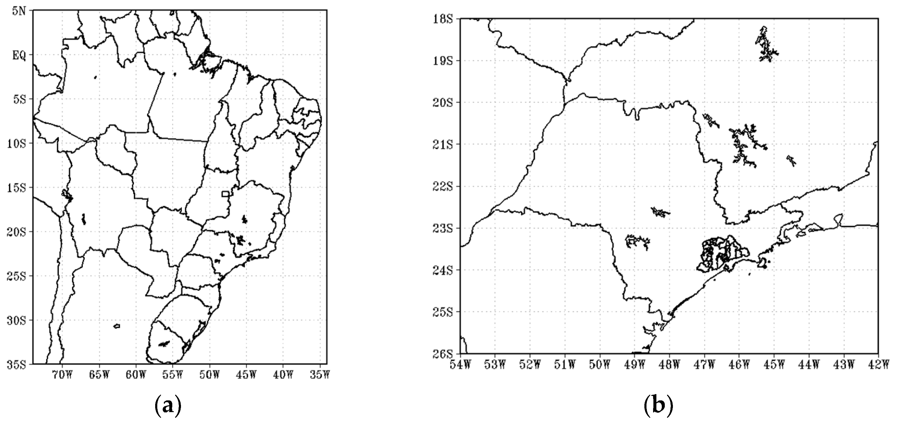
Abstract
1. Introduction
2. Materials and Methods
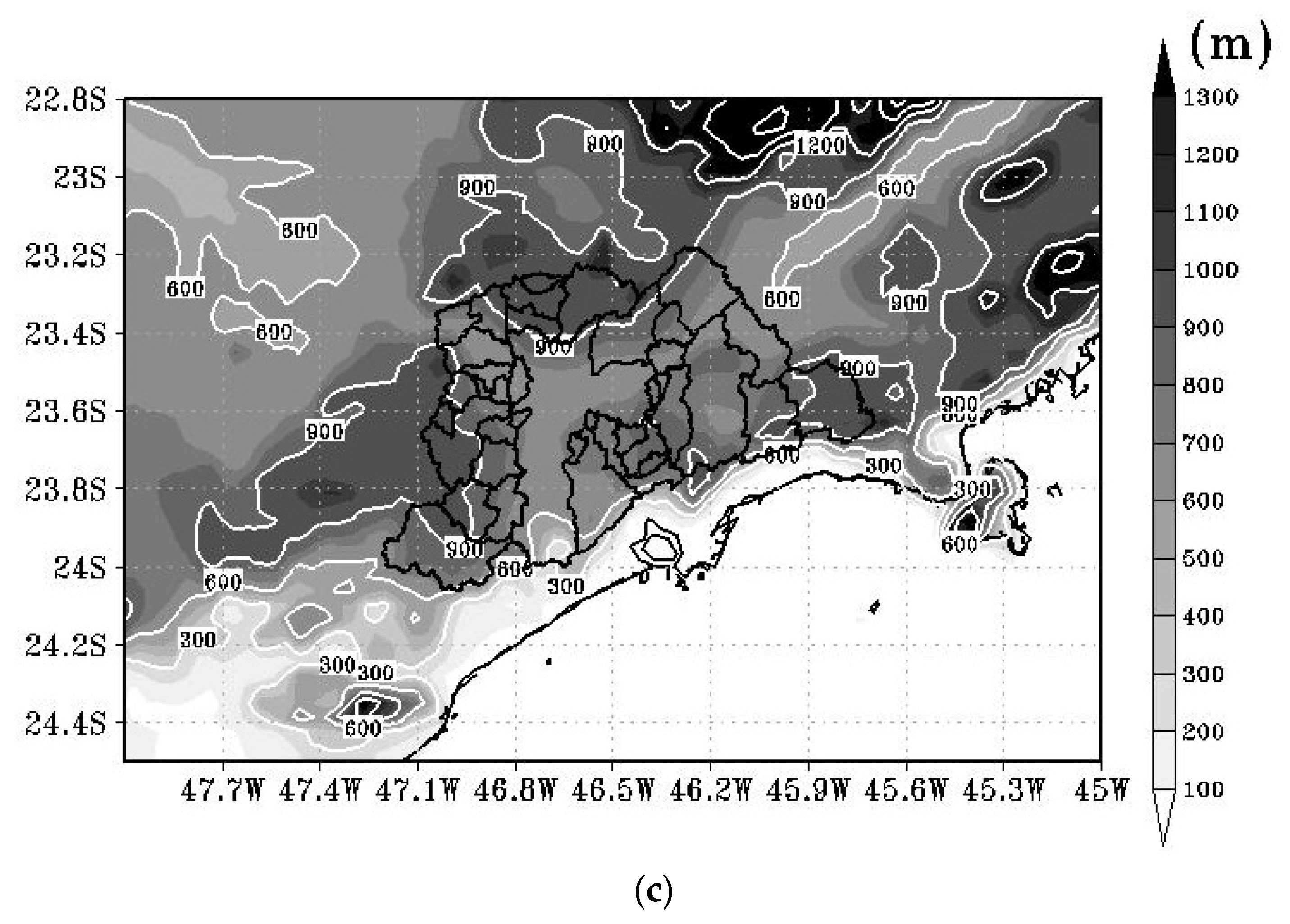
2.1. Study Area
2.2. SPM-BRAMS
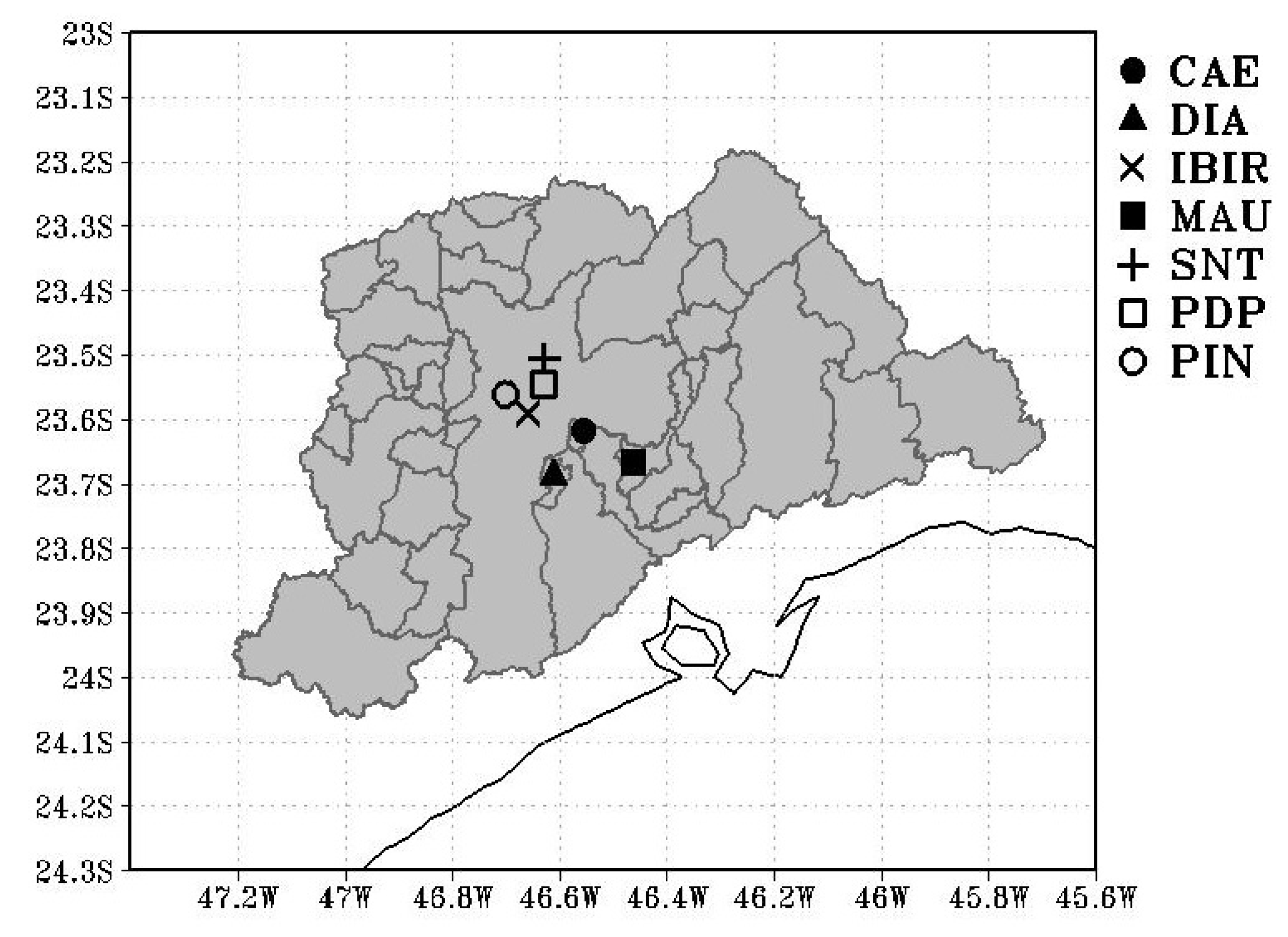
2.3. Model Evaluation
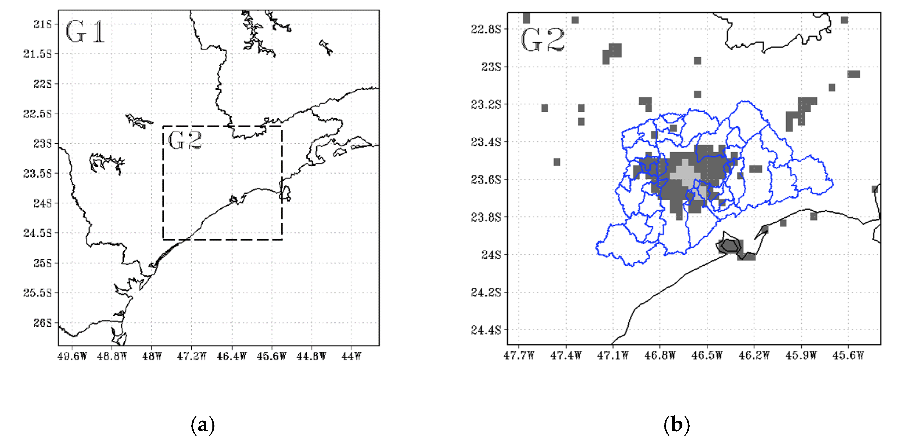
2.4. Experimental Design
3. Results
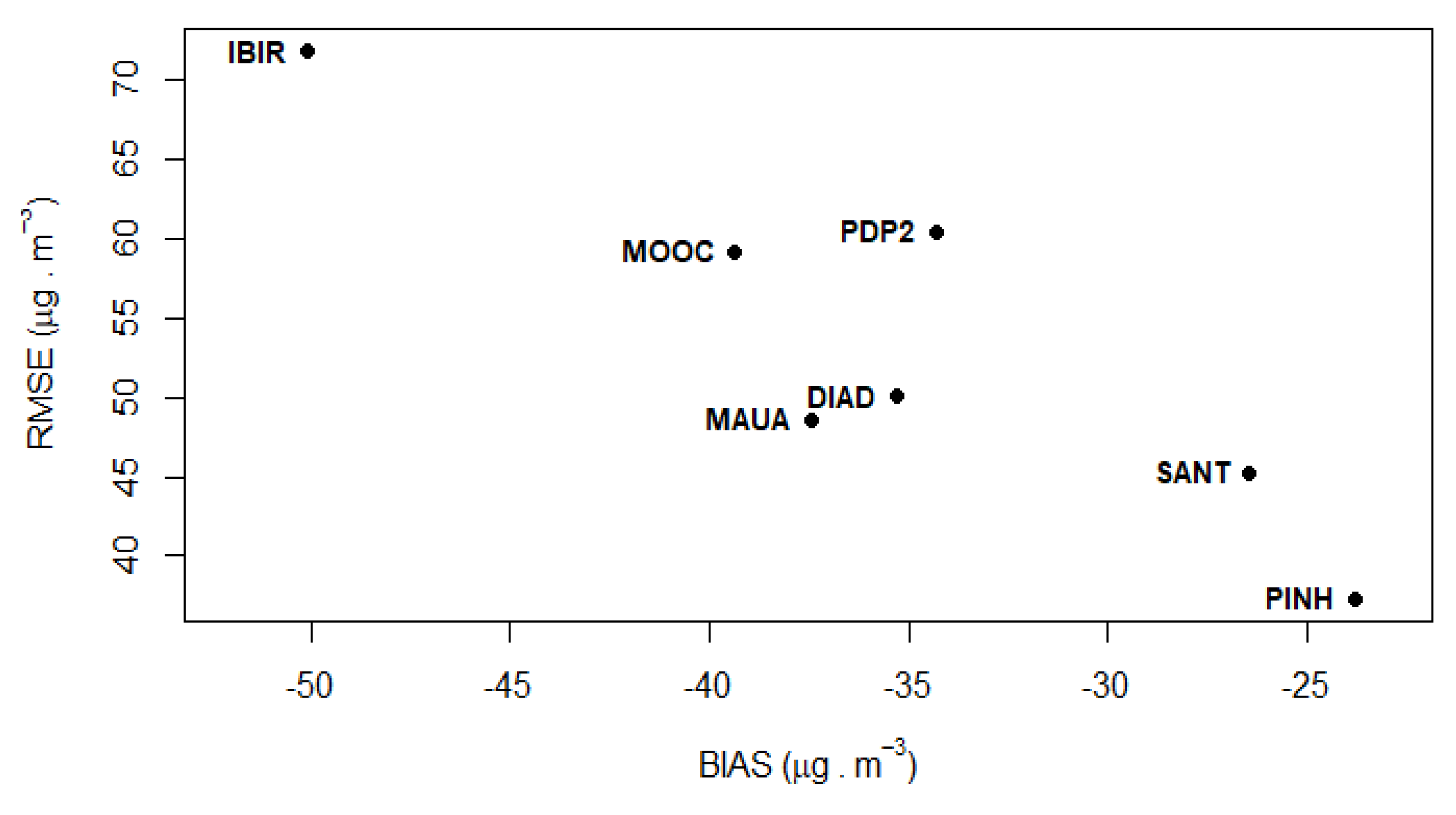
3.1. Model Evaluation
3.2. Nocturnal Ozone Experiments
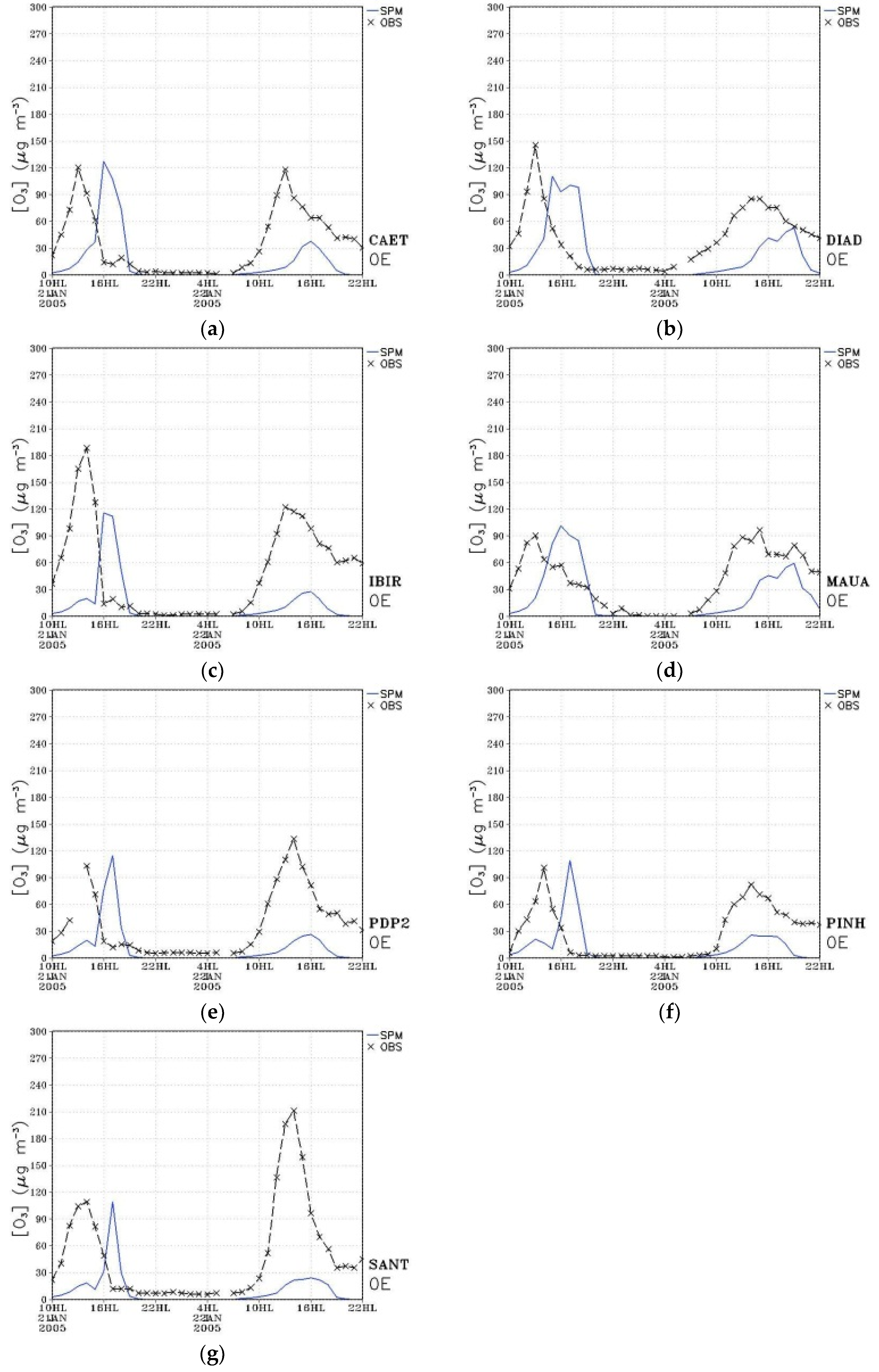
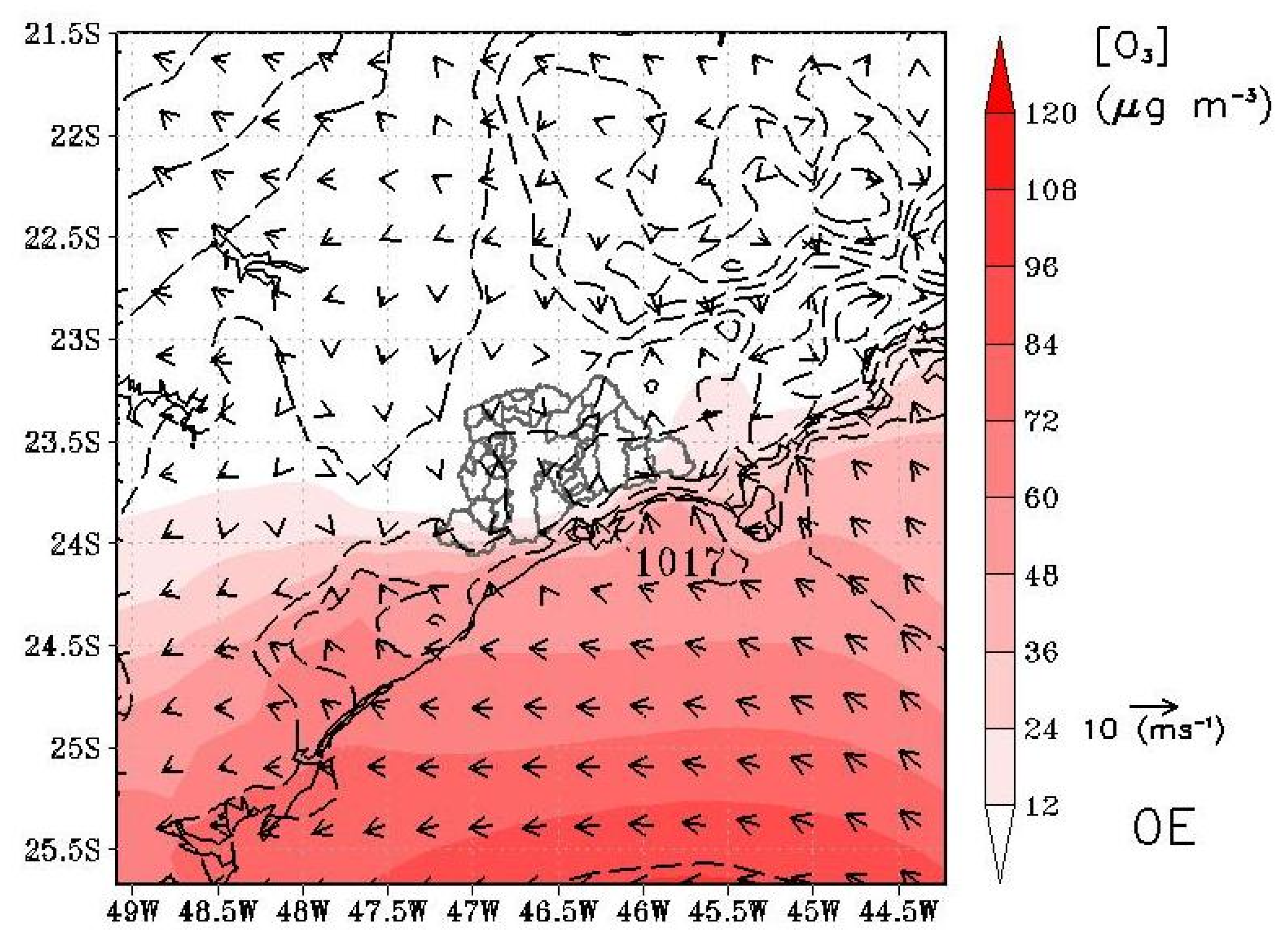
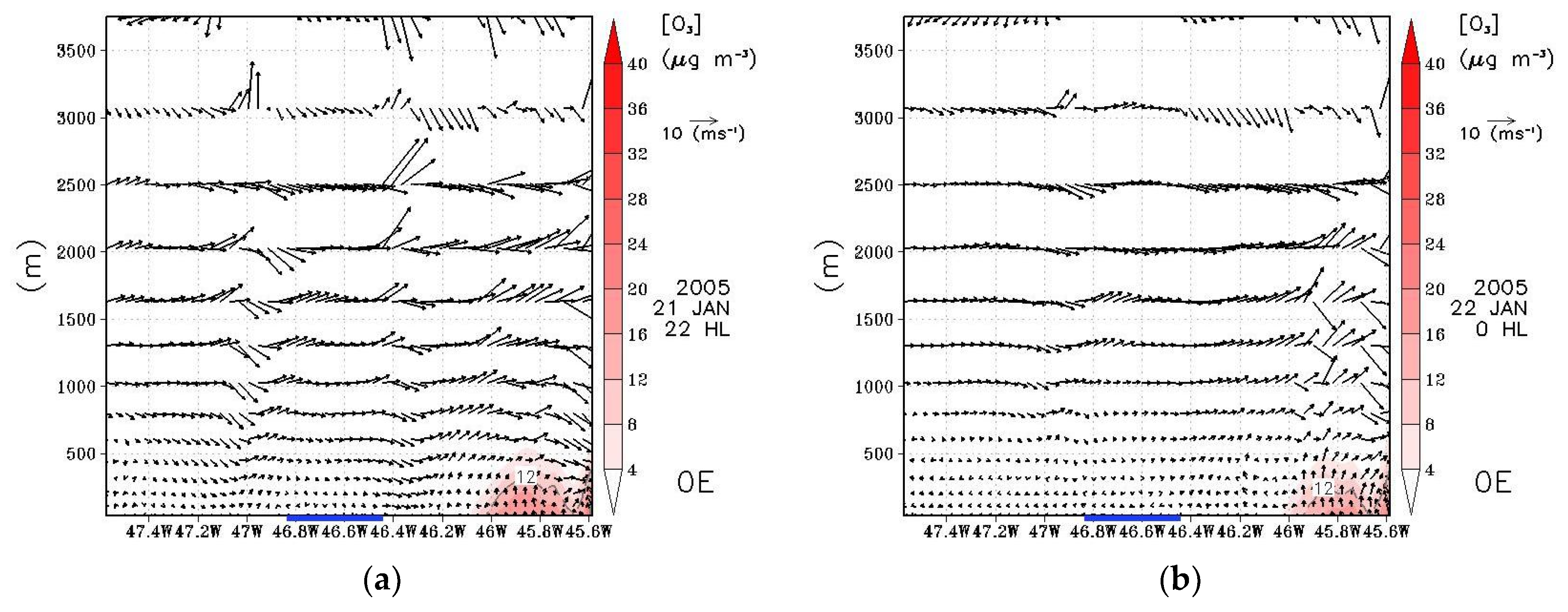
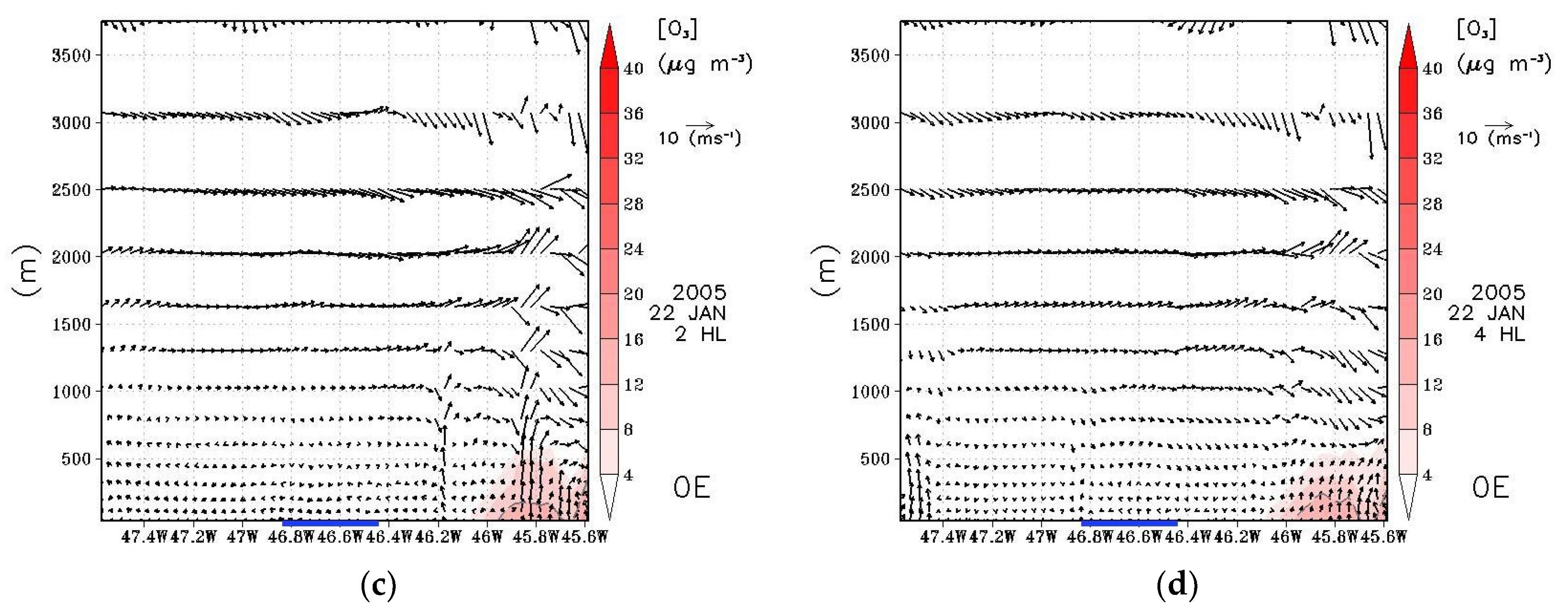
3.2.1. No Increase in Ozone Concentration (0E)
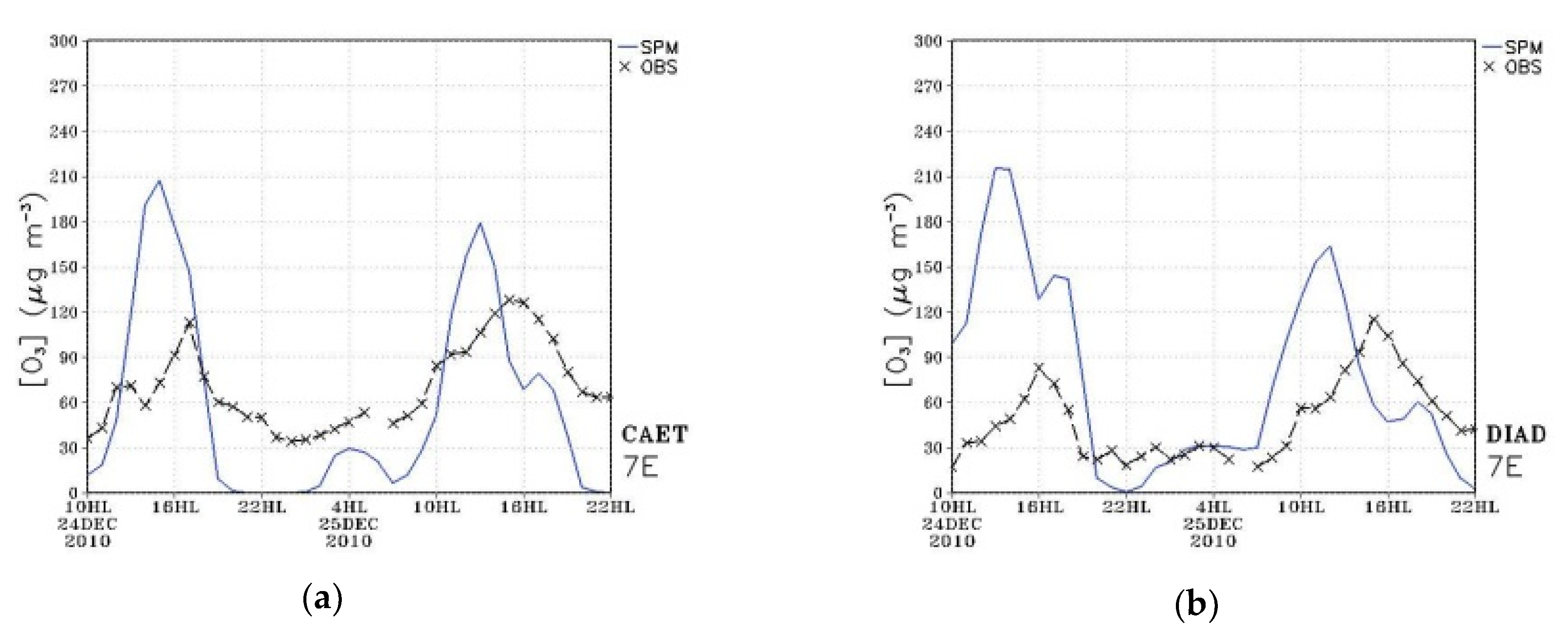
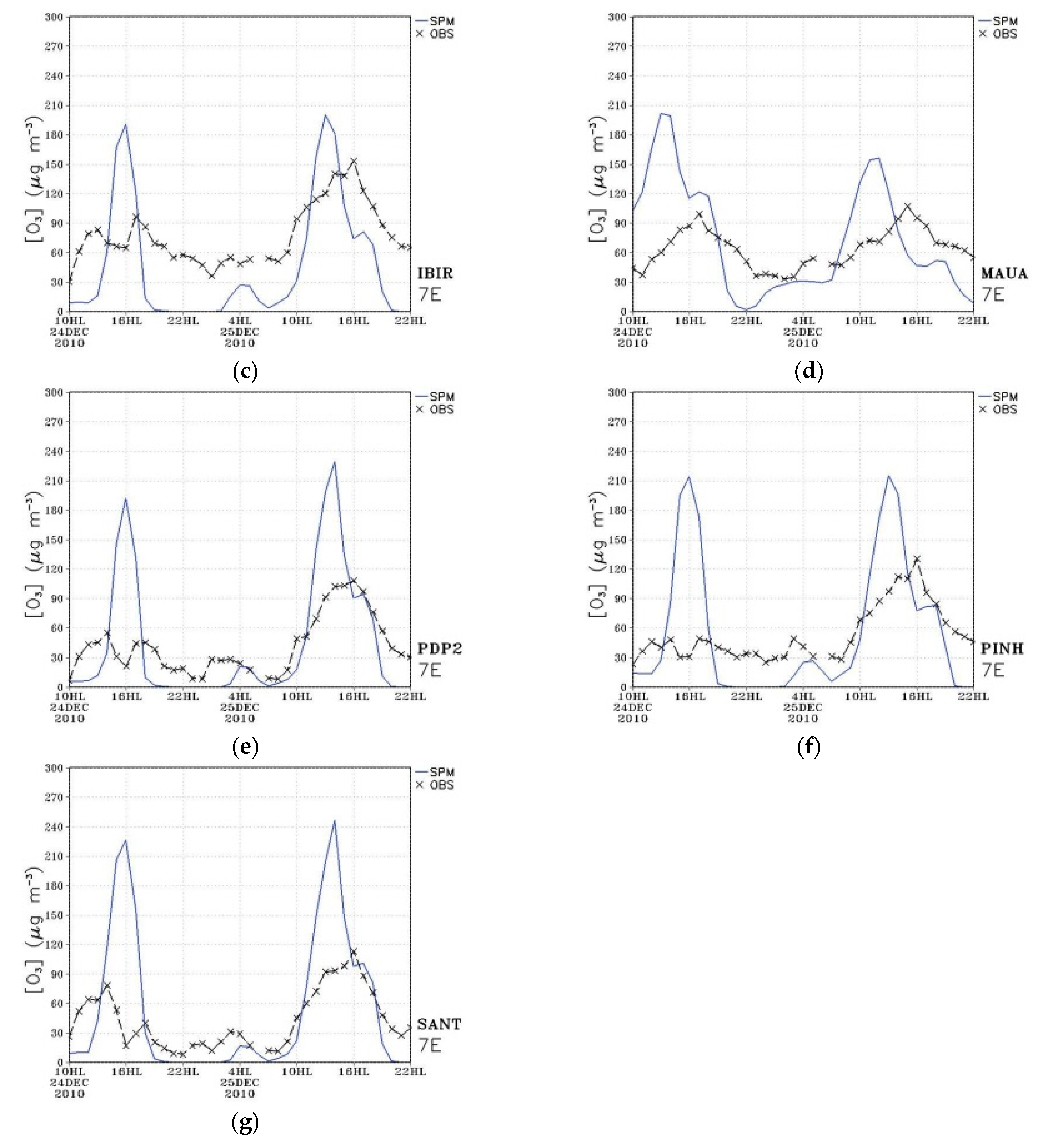
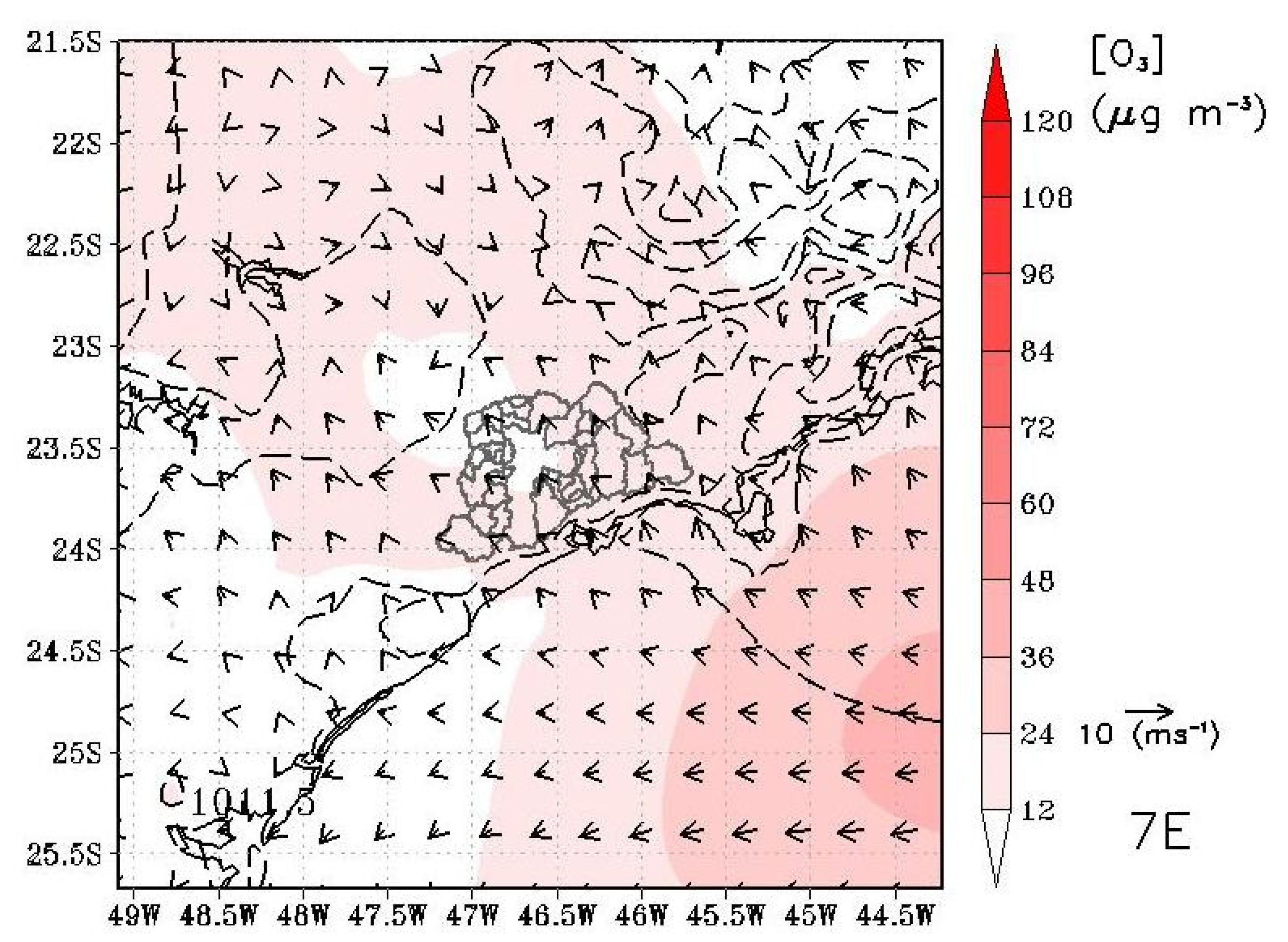
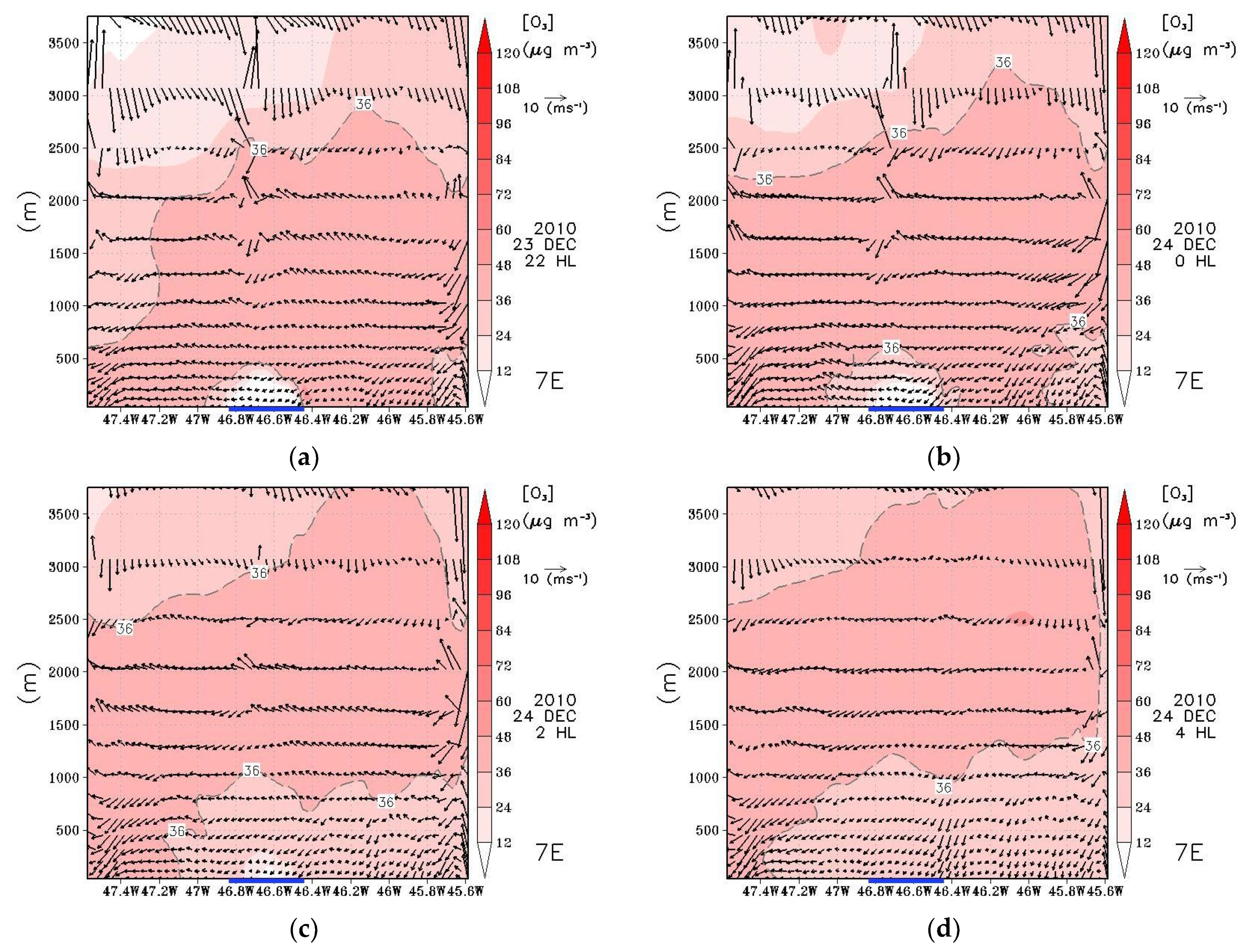
3.2.2. Increase in Ozone Concentration in All Station (7E)
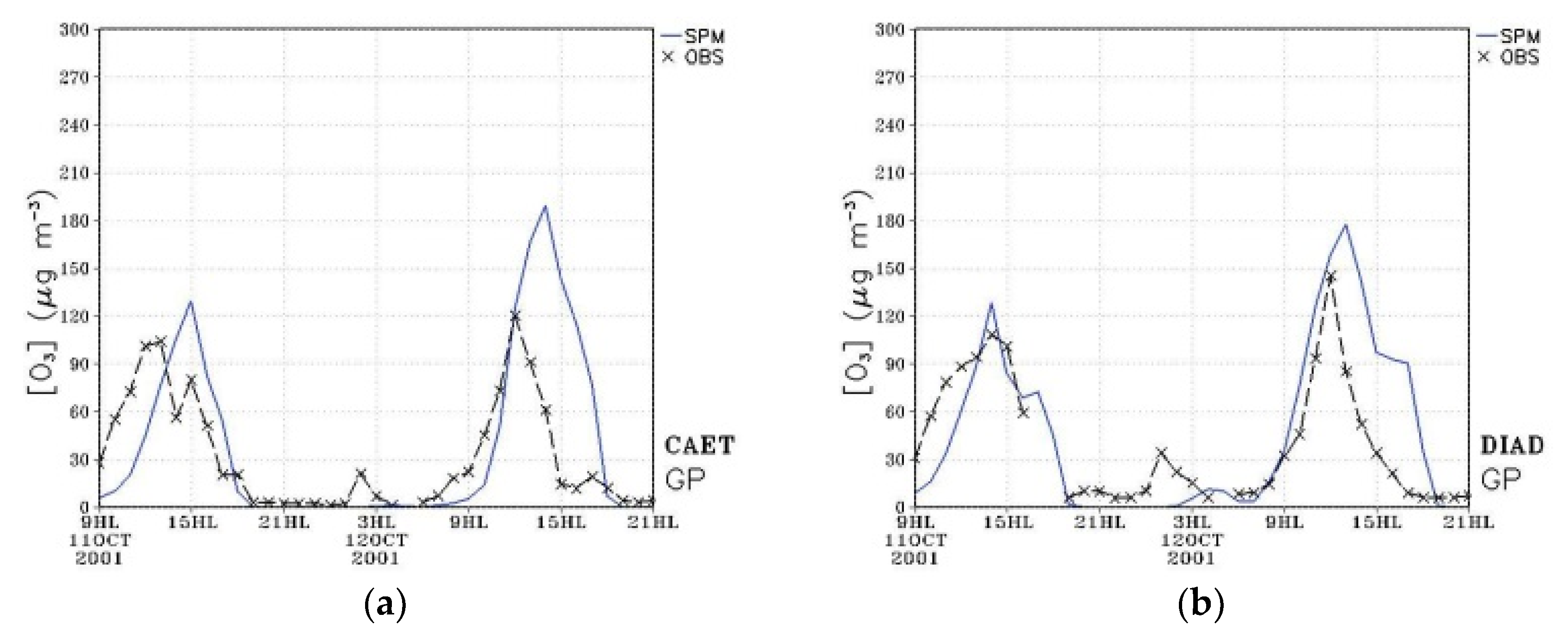
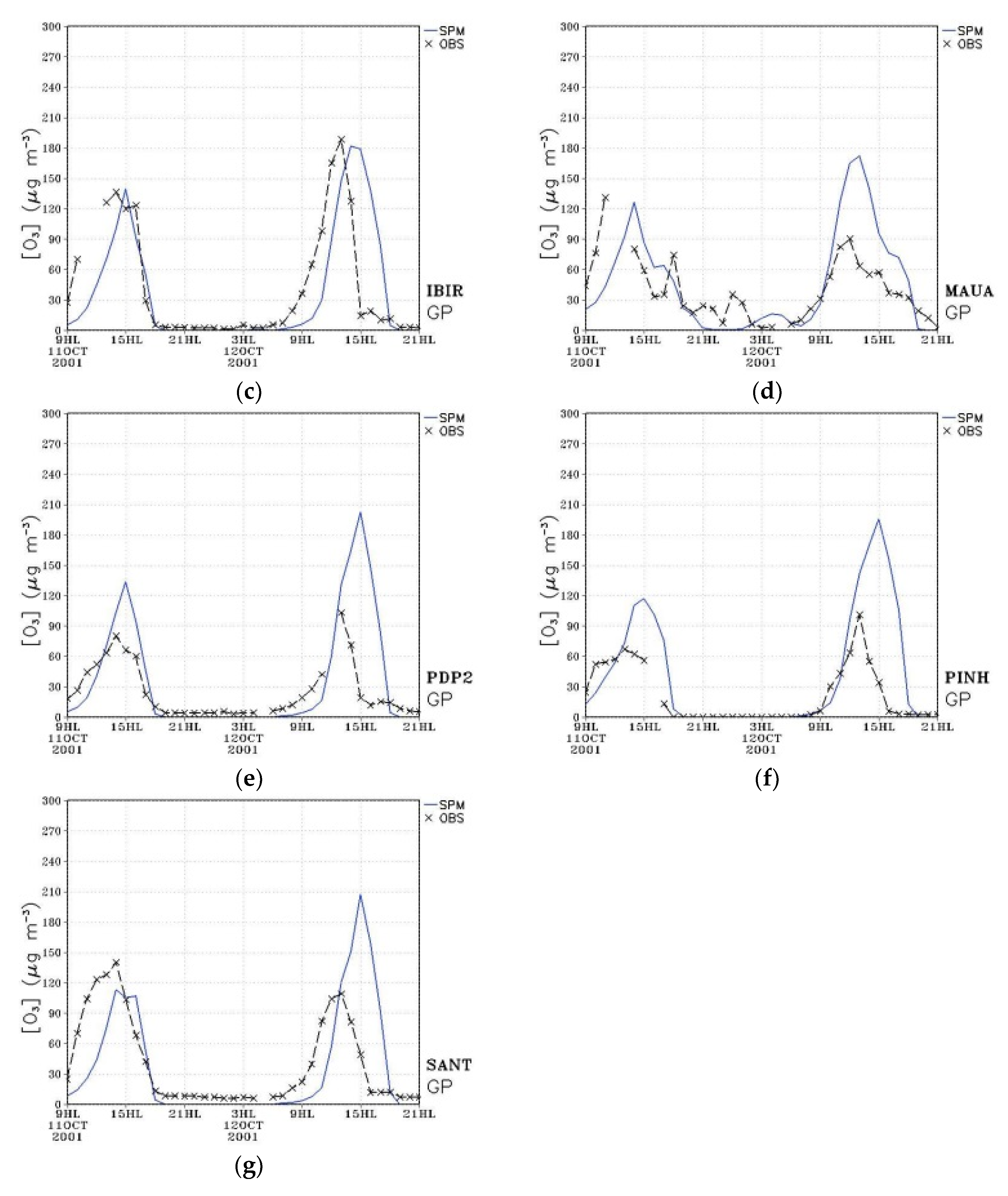
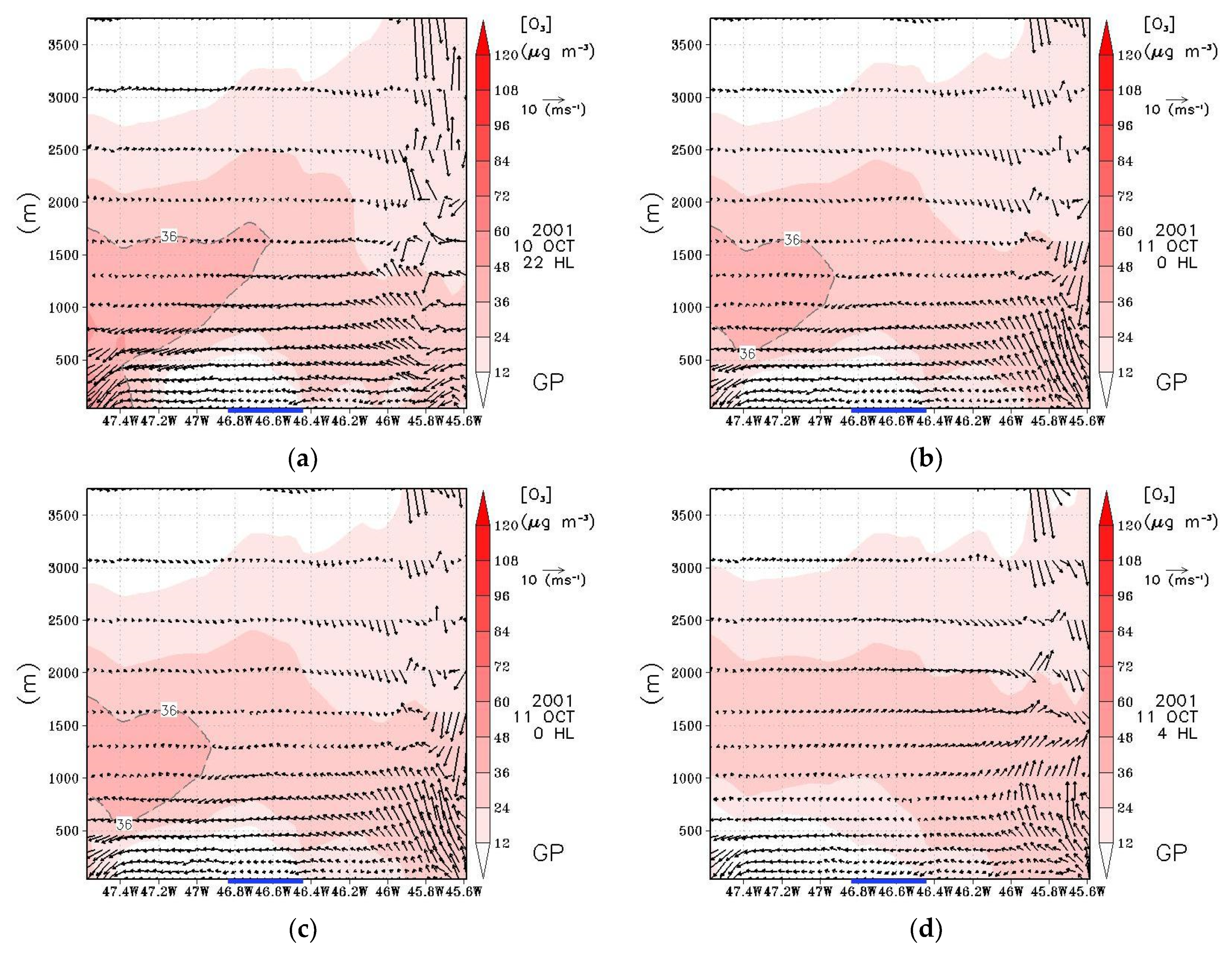
3.2.3. Increase in Ozone Concentration in Some Stations (GP)
3.2.4. Ozone Vertical Profile
4. Conclusions and Remarks
Author Contributions
Funding
Acknowledgments
Conflicts of Interest
References
- Manisalidis, I.; Stavropoulou, E.; Stavropoulos, A.; Bezirtzoglou, E. Environmental and Health Impacts of Air Pollution: A Review. Front. Public Health 2020, 8, 1–13. [Google Scholar] [CrossRef]
- Patz, J.A.; Campbell-Lendrum, D.; Holloway, T.; Foley, J.A. Impact of regional climate change on human health. Nature 2005, 438, 310–317. [Google Scholar] [CrossRef]
- Woodall, G.M.; Hoover, M.D.; Williams, R.; Benedict, K.; Harper, M.; Soo, J.C.; Jarabek, A.M.; Stewart, M.J.; Brown, J.S.; Hulla, J.E.; et al. Interpreting mobile and handheld air sensor readings in relation to air quality standards and health effect reference values: Tackling the challenges. Atmosphere 2017, 8, 182. [Google Scholar] [CrossRef]
- Bell, M.L.; Zanobetti, A.; Dominici, F. Who is More Affected by Ozone Pollution? A Systematic Review and Meta-Analysis. Am. J. Epidemiol. 2014, 180, 15–28. [Google Scholar] [CrossRef] [PubMed]
- Liana, M.; Edison, O.; Jorge, M.; Marcos, M.; Leda, A.; Guerrero, U.; Leila, M.D. Current state of air quality in major cities of Latin America. Ciência Nat. 2016, 38, 523–531. [Google Scholar] [CrossRef][Green Version]
- Peláez, L.M.G.; Santos, J.M.; Albuquerque, T.T.d.A.; Reis, N.C.; Andreão, W.L.; Andrade, M.d.F. Air quality status and trends over large cities in South America. Environ. Sci. Policy 2020, 114, 422–435. [Google Scholar] [CrossRef]
- Han, L.; Zhou, W.; Pickett, S.T.A.; Li, W.; Li, L. An optimum city size? the scaling relationship for urban population and fine particulate (PM2.5) concentration. Environ. Pollut. 2016, 208, 96–101. [Google Scholar] [CrossRef] [PubMed]
- Wang, T.; Kwok, J.Y.H. Measurement and Analysis of a Multiday Photochemical Smog Episode in the Pearl River Delta of China. J. Appl. Meteorol. 2003, 42, 404–416. [Google Scholar] [CrossRef]
- Andrade, M.D.F.; Ynoue, R.Y.; Freitas, E.D.; Todesco, E.; Vela, A.V.; Ibarra, S.; Martins, L.D.; Martins, J.A.; Carvalho, V.S.B. Air quality forecasting system for Southeastern Brazil. Front. Environ. Sci. 2015, 3, 1–14. [Google Scholar] [CrossRef]
- Samaali, M.; Moran, M.D.; Bouchet, V.S.; Pavlovic, R.; Cousineau, S.; Sassi, M. On the influence of chemical initial and boundary conditions on annual regional air quality model simulations for North America. Atmos. Environ. 2009, 43, 4873–4885. [Google Scholar] [CrossRef]
- Balzarini, A.; Pirovano, G.; Honzak, L.; Žabkar, R.; Curci, G.; Forkel, R.; Hirtl, M.; San José, R.; Tuccella, P.; Grell, G.A. WRF-Chem model sensitivity to chemical mechanisms choice in reconstructing aerosol optical properties. Atmos. Environ. 2015, 115, 604–619. [Google Scholar] [CrossRef]
- Vara-Vela, A.; Andrade, M.F.; Kumar, P.; Ynoue, R.Y.; Muñoz, A.G. Impact of vehicular emissions on the formation of fine particles in the Sao Paulo Metropolitan Area: A numerical study with the WRF-Chem model. Atmos. Chem. Phys. 2016, 16, 777–797. [Google Scholar] [CrossRef]
- Mateos, A.C.; Amarillo, A.C.; Busso, I.T.; Carreras, H.A. Influence of Meteorological Variables and Forest Fires Events on Air Quality in an Urban Area (Córdoba, Argentina). Arch. Environ. Contam. Toxicol. 2019, 77, 171–179. [Google Scholar] [CrossRef] [PubMed]
- Romero, H.; Ihl, M.; Rivera, A.; Zalazar, P.; Azocar, P. Rapid urban growth, land-use changes and air pollution in Santiago, Chile. Atmos. Environ. 1999, 33, 4039–4047. [Google Scholar] [CrossRef]
- Mar, K.A.; Ojha, N.; Pozzer, A.; Butler, T.M. Ozone air quality simulations with WRF-Chem (v3.5.1) over Europe: Model evaluation and chemical mechanism comparison. Geosci. Model Dev. 2016, 9, 3699–3728. [Google Scholar] [CrossRef]
- Ren, X.; Mi, Z.; Georgopoulos, P.G. Comparison of Machine Learning and Land Use Regression for fine scale spatiotemporal estimation of ambient air pollution: Modeling ozone concentrations across the contiguous United States. Environ. Int. 2020, 142, 105827. [Google Scholar] [CrossRef]
- Gramsch, E.; Cereceda-Balic, F.; Oyola, P.; von Baer, D. Examination of pollution trends in Santiago de Chile with cluster analysis of PM10 and Ozone data. Atmos. Environ. 2006, 40, 5464–5475. [Google Scholar] [CrossRef]
- Khan, B.A.; de Freitas, C.R.; Shooter, D. Application of synoptic weather typing to an investigation of nocturnal ozone concentration at a maritime location, New Zealand. Atmos. Environ. 2007, 41, 5636–5646. [Google Scholar] [CrossRef]
- Alp, K.; Hanedar, A.O. Determination of transport processes of nocturnal ozone in Istanbul atmosphere. Int. J. Environ. Pollut. 2009, 39, 213. [Google Scholar] [CrossRef]
- Zhu, X.; Ma, Z.; Li, Z.; Wu, J.; Guo, H.; Yin, X.; Ma, X.; Qiao, L. Impacts of meteorological conditions on nocturnal surface ozone enhancement during the summertime in Beijing. Atmos. Environ. 2020, 225, 117368. [Google Scholar] [CrossRef]
- Ghosh, D.; Lal, S.; Sarkar, U. High nocturnal ozone levels at a surface site in Kolkata, India: Trade-off between meteorology and specific nocturnal chemistry. Urban Clim. 2013, 5, 82–103. [Google Scholar] [CrossRef]
- Godowitch, J.M.; Gilliland, A.B.; Draxler, R.R.; Rao, S.T. Modeling assessment of point source NOx emission reductions on ozone air quality in the eastern United States. Atmos. Environ. 2008, 42, 87–100. [Google Scholar] [CrossRef]
- Sicard, P.; Serra, R.; Rossello, P. Spatiotemporal trends in ground-level ozone concentrations and metrics in France over the time period 1999-2012. Environ. Res. 2016, 149, 122–144. [Google Scholar] [CrossRef] [PubMed]
- IBGE Censo Demográfico: Características da População—Amostra. Available online: https://censo2010.ibge.gov.br/resultados.html (accessed on 16 October 2020).
- Nair, K.N.; Freitas, E.D.; Sãnchez-Ccoyllo, O.R.; Silva Dias, M.a.F.; Silva Dias, P.L.; Andrade, M.F.; Massambani, O. Dynamics of urban boundary layer over São Paulo associated with mesoscale processes. Meteorol. Atmos. Phys. 2004, 86, 87–98. [Google Scholar] [CrossRef]
- Andrade, M.d.F.; Kumar, P.; de Freitas, E.D.; Ynoue, R.Y.; Martins, J.; Martins, L.D.; Nogueira, T.; Perez-Martinez, P.; de Miranda, R.M.; Albuquerque, T.; et al. Air quality in the megacity of São Paulo: Evolution over the last 30 years and future perspectives. Atmos. Environ. 2017, 159, 66–82. [Google Scholar] [CrossRef]
- Freitas, S.R.; Panetta, J.; Longo, K.M.; Rodrigues, L.F.; Moreira, D.S.; Rosário, N.E.; Silva Dias, P.L.; Silva Dias, M.A.F.; Souza, E.P.; Freitas, E.D.; et al. The Brazilian developments on the Regional Atmospheric Modeling System (BRAMS 5.2): An integrated environmental model tuned for tropical areas. Geosci. Model Dev. 2017, 10, 189–222. [Google Scholar] [CrossRef] [PubMed]
- Cotton, W.R.; Pielke, R.A., Sr.; Walko, R.L.; Liston, G.E.; Tremback, C.J.; Jiang, H.; McAnelly, R.L.; Harrington, J.Y.; Nicholls, M.E.; Carrio, G.G.; et al. RAMS 2001: Current status and future directions. Meteorol. Atmos. Phys. 2003, 82, 5–29. [Google Scholar] [CrossRef]
- Walko, R.L.; Band, L.E.; Baron, J.; Kittel, T.G.F.; Lammers, R.; Lee, T.J.; Ojima, D.; Pielke, R.A.; Taylor, C.; Tague, C.; et al. Coupled Atmosphere–Biophysics–Hydrology Models for Environmental Modeling. J. Appl. Meteorol. 2000, 39, 931–944. [Google Scholar] [CrossRef]
- Masson, V. A physically-based scheme for the urban energy budget in atmospheric models. Bound. Layer Meteorol. 2000, 94, 357–397. [Google Scholar] [CrossRef]
- Daley, R. (Ed.) Atmospheric Data Analysis; Cambridge University Press: Cambridge, UK, 1991. [Google Scholar]
- Morais, M.V.B.; Freitas, E.D.; Marciotto, E.R.; Guerrero, V.V.U.; Martins, L.D.; Martins, J.A. Implementation of observed sky-view factor in a mesoscale model for sensitivity studies of the urban meteorology. Sustainability 2018, 10, 2183. [Google Scholar] [CrossRef]
- Freitas, E.D.; Martins, L.D.; Silva Dias, P.L.; Andrade, M.F. A simple photochemical module implemented in RAMS for tropospheric ozone concentration forecast in the metropolitan area of São Paulo, Brazil: Coupling and validation. Atmos. Environ. 2005, 39, 6352–6361. [Google Scholar] [CrossRef]
- Wang, L.; Zhang, Y.; Wang, K.; Zheng, B.; Zhang, Q.; Wei, W. Application of Weather Research and Forecasting Model with Chemistry (WRF/Chem) over northern China: Sensitivity study, comparative evaluation, and policy implications. Atmos. Environ. 2014. [Google Scholar] [CrossRef]
- Morais, M.V.B.; de Freitas, E.D.; Guerrero, V.V.U.; Martins, L.D. A modeling analysis of urban canopy parameterization representing the vegetation effects in the megacity of São Paulo. Urban Clim. 2016, 17, 102–115. [Google Scholar] [CrossRef]
- CETESB. Qualidade do Ar no Estado de São Paulo 2010; CETESB: São Paulo, Brazil, 2011. [Google Scholar]
- Kalnay, E.; Kanamitsu, M.; Kistler, R.; Collins, W.; Deaven, D.; Gandin, L.; Iredell, M.; Saha, S.; White, G.; Woollen, J.; et al. The NCEP/NCAR 40-year reanalysis project. Bull. Am. Meteorol. Soc. 1996, 77, 437–472. [Google Scholar] [CrossRef]
- Franco, D.M.P.; Andrade, M.d.F.; Ynoue, R.Y.; Ching, J. Effect of Local Climate Zone (LCZ) classification on ozone chemical transport model simulations in Sao Paulo, Brazil. Urban Clim. 2019, 27, 293–313. [Google Scholar] [CrossRef]
- Martins, L.D.; Wikuats, C.F.H.; Capucim, M.N.; Almeida, D.S.; Costa, S.C.; Albuquerque, T.; Barreto Carvalho, V.S.; Freitas, E.D.; de Fátima Andrade, M.; Martins, J.A. Extreme value analysis of air pollution data and their comparison between two large urban regions of South America. Weather Clim. Extrem. 2017, 18, 44–54. [Google Scholar] [CrossRef]
- Carvalho, V.S.B.; Freitas, E.D.; Martins, L.D.; Martins, J.A.; Mazzoli, C.R.; de Fátima Andrade, M. Air quality status and trends over the Metropolitan Area of São Paulo, Brazil as a result of emission control policies. Environ. Sci. Policy 2015, 47, 68–79. [Google Scholar] [CrossRef]
- Alvim, D.S.; Gatti, L.V.; Corrêa, S.M.; Chiquetto, J.B.; Santos, G.M.; de Souza Rossatti, C.; Pretto, A.; Rozante, J.R.; Figueroa, S.N.; Pendharkar, J.; et al. Determining VOCs reactivity for ozone forming potential in the megacity of São Paulo. Aerosol Air Qual. Res. 2018, 18, 2460–2474. [Google Scholar] [CrossRef]


Publisher’s Note: MDPI stays neutral with regard to jurisdictional claims in published maps and institutional affiliations. |
© 2021 by the authors. Licensee MDPI, Basel, Switzerland. This article is an open access article distributed under the terms and conditions of the Creative Commons Attribution (CC BY) license (http://creativecommons.org/licenses/by/4.0/).
Share and Cite
Urbina Guerrero, V.V.; Morais, M.V.B.d.; Freitas, E.D.d.; Martins, L.D. Numerical Study of Meteorological Factors for Tropospheric Nocturnal Ozone Increase in the Metropolitan Area of São Paulo. Atmosphere 2021, 12, 287. https://doi.org/10.3390/atmos12020287
Urbina Guerrero VV, Morais MVBd, Freitas EDd, Martins LD. Numerical Study of Meteorological Factors for Tropospheric Nocturnal Ozone Increase in the Metropolitan Area of São Paulo. Atmosphere. 2021; 12(2):287. https://doi.org/10.3390/atmos12020287
Chicago/Turabian StyleUrbina Guerrero, Viviana Vanesa, Marcos Vinicius Bueno de Morais, Edmilson Dias de Freitas, and Leila Droprinchinski Martins. 2021. "Numerical Study of Meteorological Factors for Tropospheric Nocturnal Ozone Increase in the Metropolitan Area of São Paulo" Atmosphere 12, no. 2: 287. https://doi.org/10.3390/atmos12020287
APA StyleUrbina Guerrero, V. V., Morais, M. V. B. d., Freitas, E. D. d., & Martins, L. D. (2021). Numerical Study of Meteorological Factors for Tropospheric Nocturnal Ozone Increase in the Metropolitan Area of São Paulo. Atmosphere, 12(2), 287. https://doi.org/10.3390/atmos12020287