Influence of Random Forest Hyperparameterization on Short-Term Runoff Forecasting in an Andean Mountain Catchment

Abstract

The Random Forest (RF) algorithm, a decision-tree-based technique, has become a promising approach for applications addressing runoff forecasting in remote areas. This machine learning approach can overcome the limitations of scarce spatio-temporal data and physical parameters needed for process-based hydrological models. However, the influence of RF hyperparameters is still uncertain and needs to be explored. Therefore, the aim of this study is to analyze the sensitivity of RF runoff forecasting models of varying lead time to the hyperparameters of the algorithm. For this, models were trained by using (a) default and (b) extensive hyperparameter combinations through a grid-search approach that allow reaching the optimal set. Model performances were assessed based on the R², %Bias, and RMSE metrics. We found that: (i) The most influencing hyperparameter is the number of trees in the forest, however the combination of the depth of the tree and the number of features hyperparameters produced the highest variability-instability on the models. (ii) Hyperparameter optimization significantly improved model performance for higher lead times (12- and 24-h). For instance, the performance of the 12-h forecasting model under default RF hyperparameters improved to R² = 0.41 after optimization (gain of 0.17). However, for short lead times (4-h) there was no significant model improvement (0.69 < R² < 0.70). (iii) There is a range of values for each hyperparameter in which the performance of the model is not significantly affected but remains close to the optimal. Thus, a compromise between hyperparameter interactions (i.e., their values) can produce similar high model performances. Model improvements after optimization can be explained from a hydrological point of view, the generalization ability for lead times larger than the concentration time of the catchment tend to rely more on hyperparameterization than in what they can learn from the input data. This insight can help in the development of operational early warning systems.

1. Introduction

Among the machine learning techniques most widely used in different fields of science, the Random Forest (RF) [1] is one of the most useful and best performing for both classification and regression applications [2,3,4,5,6,7,8,9,10]. Nonetheless, specifically used for timeseries data, there are few RF applications in the current literature [11]. The success of the RF algorithm is associated to its self-assembling nature, where a forest represents a robust non-linear model derived from a large number of individual models (trees) [12]. Robustness is explained by the capability of the RF algorithm to deal with datasets with specific problems such as missing and/or outliers values, non-standardized, and unbalanced in relatively high dimensional spaces [7]. Moreover, the RF algorithm allows complex interactions between input features, and this results in a relative well handling of model overfitting [3]. In addition to the aforementioned reasons, a crucial aspect that motivates the use of the RF algorithm over other machine learning (ML) techniques is the possibility to produce estimates on the importance of each feature in the feature space [13]. In other words, it allows us to identify which features are the most relevant when executing the forecasts. For the majority of studies, this information is as important as the prediction results [14].

The RF hyperparameters enable controlling the structure of decision trees (e.g., depth of each tree, maximum number of leaf nodes in the tree, and minimum number of samples in the leaf nodes), and diversity between trees in the forest (number of trees, number of variables to consider at each division, and percentage of total data employed in the construction of each tree) [1,14,15,16]. Other more specialized hyperparameters are focused on controlling how internal divisions are performed in each tree (e.g., quality of a division or the minimum number of samples required to divide an internal node).

In environmental applications, the RF algorithm has been used to simulate variables such as rainfall, runoff, water level, groundwater potential, and pollutant concentrations, among others [3,4,5,6,7,8,17,18,19,20,21,22]. From these applications, runoff forecasting in mountainous regions is increasingly gaining the attention of hydrologists. This is because the RF algorithm has demonstrated an improved predictive ability and a lower number of hyperparameters to calibrate when compared to physical-based models [23,24]. Moreover, the use of RF is convenient for addressing data limitation issues in mountainous regions, which arise from sparse monitoring networks and extreme spatio-temporal variability of runoff-driving forces (precipitation, snow melting, topography, soil moisture, etc.) [3,19,22,25,26].

Although extensive research has been carried out on identifying the most relevant input features [27,28], no single study exists that focuses on the influence of RF hyperparameters in the performance of runoff forecasting models. This is because prior studies have shown that in most cases, contrary to other ML techniques, the RF algorithm works fairly well with default values [14,29,30]. However, this hinders a proper exploitation of the algorithm. In contrast, optimal fitting results can be obtained through hyperparameter optimization [31,32]. This is argued in the study of Bergstra and Bengio [33], where it is stated that for most datasets types, only a few hyperparameters influences model performance, but there is a different combination of hyperparameters influencing each type of dataset. In other words, the hyperparameters with the highest sensitivity to the RF model might differ between applications. To date, there is no report of an exhaustive RF architecture study performed for regression problems in hydrology such as runoff forecasting.

Instead, most of the runoff modeling and forecasting studies solely explore the parameter that defines the number of trees in the forest [3,25,26], or even directly focus on the feature (predictor) selection process without consideration of RF hyperparameters [34]. This has resulted in a poor understanding for non-specialized machine learning hydrologists, and incomplete exploitation of the algorithm in terms of model performance. Moreover, scrutinizing RF models built up under different hyperparameter choices is a rare exercise considering the increasing efforts to develop new ML methods. Therefore, given the great popularity gained by RF models during the last decades, it becomes crucial to investigate the behavior of the RF model under different hyperparameter values.

Therefore, the objective of this study is to identify the most important RF hyperparameters and to evaluate their impact on the performance of short-term runoff forecasting models in a mountain catchment. To determine whether this impact is related to the lead time of forecasting, we developed models for forecast horizons of 4, 12, and 24 h.

2. Materials and Methods

2.1. Study Site

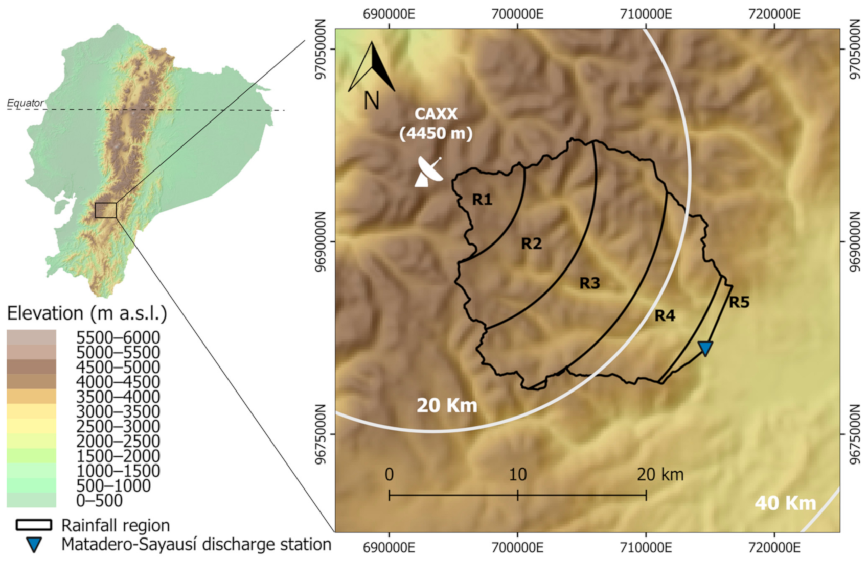
The study was conducted in the Tomebamba catchment, upstream of the city of Cuenca (aprox. 0.6 million inhabitants), in the Ecuadorian Andes. The Tomebamba is a 300-km² catchment with elevations ranging from 2600 to 4200 m above sea level (m a.s.l.) (Figure 1). The mean annual rainfall is 850 and 1100 mm in the lower and upper parts of the catchment, respectively. Two rainy seasons have been identified, a first one during March-April-May, and a second shorter one in October. The importance of the Tomebamba catchment is related to its water-supplier role for Cuenca. However, the catchment is also responsible for periodically flooding parts of the city.

2.2. Instruments and Data

For modelling, we relied on precipitation and runoff data for the Tomebamba catchment. For runoff, we used hourly time series obtained from the Matadero-Sayausí hydrological station. This station is located at the outlet of the catchment, where the river enters the city of Cuenca (Figure 1). Regarding precipitation to force the hydrological model, we used information retrieved from an X-band meteorological radar, which is located nearby the upper part of the catchment, on the Paragüillas peak (4450 m a.s.l.). Radar data comprise reflectivity polar images with a temporal resolution of 5 min, and a spatial resolution of 100m at a scan azimuth angle of 2 degrees. Concurrent data for runoff and precipitation is available for more than two years (from March 2015 to June 2017).

Considering the high resolution data of the radar, and the associated computational cost, we reduced the amount of input data to the models. For this, the catchment was divided into 5 concentric elevation bands (Figure 1) by following the methodology of [22]. Thus, the native radar reflectivity (dBZ) was used to represent the precipitation as input for the model. Here, the areal average precipitation registered at each region, at each time step was calculated for deriving the timeseries. Moreover, considering that we aim to develop hourly models, radar data were aggregated to an hourly scale. Therefore, five different hourly time series were derived, one for each elevation band.

Once processed, the complete dataset was split up into two subsets, one for training-validation and one for testing activities of the RF model. The training-validation subset was exploited within a 3-fold cross-validation scheme. This means that for each iteration (3 in total), 2 out of 3 folds were used for training, and the remaining fold was used for validation purposes. For each validation fold, we calculate the efficiency metrics further described in Section 2.5. The averaged efficiency metrics obtained from all three iterations will be reported as the metrics corresponding to the training-validation stage. Moreover, for the training-validation and testing subsets, we used continuous and independent windows of the complete timeseries. In this way, we avoid adding runoff information of the test subset during the training-validation phase. This is because this information should remain unknown for a proper model evaluation on the testing subset. Data available between January 2015 and June 2016 were used for training-validation and data available between July 2016 and June 2017 for testing.

2.3. Random Forest and Hyperparameters

The Random Forest (RF) for regression is an assembler-like algorithm that averages the responses of a finite number of regression trees to infer the prediction of a target variable [1,35]. A single regression tree represents a set of conditions or constraints that are hierarchically organized and applied successively from the root to a leaf in a tree [7]. Basically, each tree is built from a root node which is divided into 2 or more sub nodes iteratively. To determine the division of the nodes in regression problems, MSE is used as the objective function to determine the ‘best split’ in each step.

For the construction of trees, RF uses a technique known as bagging. Bagging implies that each individual tree is randomly created from a subset of data (roughly two-thirds of the corresponding training subset), leaving the remaining data for internal validation (out-of-bag error). Bagging allows (i) to increase the diversity of the trees and thus avoid the correlation of the different trees, (ii) to increase the stability of the model, and (iii) to improve the prediction precision [1]. A more detailed explanation of the RF algorithm can be found in [1].

Although the out-of-bag error is argued to be a proper measurement of model efficiency, we decided to keep independent datasets for model assessment during the training-validation and testing phases. This is because in hydrological studies it is a common practice to split the time series into calibration—for training the model—and independent validation—for testing the model. The logic behind this practice relies on the continuous nature of processes generating runoff. For this reason, we decided to use continuous windows of the timeseries for splitting our dataset into training-validation and test subsets. In other words, we aimed to train, validate, and test our models with independent runoff events. By doing this, we ensure a proper evaluation of the robustness and generalization capability of the model.

The RF algorithm has been implemented in several programming languages (e.g., Python and R), and thus, it has several hyperparameters with names that might differ between libraries. In this study, we specifically use the implementation of Python’s scikit-learn library [36] (version 0.21) that contains the hyperparameters defined in

Table 1. Description of used hyperparameters.

Hyperparameter	Description	Range	Default Value
criterion	The metric to measure the quality of a split	[mean absolute error, mean squared error]	mean squared error
max_depth	The maximum depth that can reach a tree.	From 1 to number of training samples	‘None’ (Until all leaves are pure)
max_features	The maximum number of features that is allowed to try in individual tree.	From 1 to total number of features	Total number of features
max_leaf_nodes	The maximum number of leaf nodes	From 1 to unlimited number of leaf nodes	Unlimited number of leaf nodes
max_samples	The maximum number of samples to take to train each tree	From 1% to 100%	All samples
min_samples_leaf	The minimum number of samples allowed to be a leaf node.	From 1 to total number of samples	1
min_samples_split	The minimum number of samples allowed to split an internal node	From 2 to total number of samples	2
n_estimators	The total number of trees in the forest.	From 1 to unlimited	100

.

As previously mentioned, the RF has shown good performance with most hyperparameters with their default values [14]. In this study, we focused only on the hyperparameters that when optimized represent an improvement in the predictive power of the model. Therefore, a local sensitivity analysis was previously performed to identify these hyperparameters.

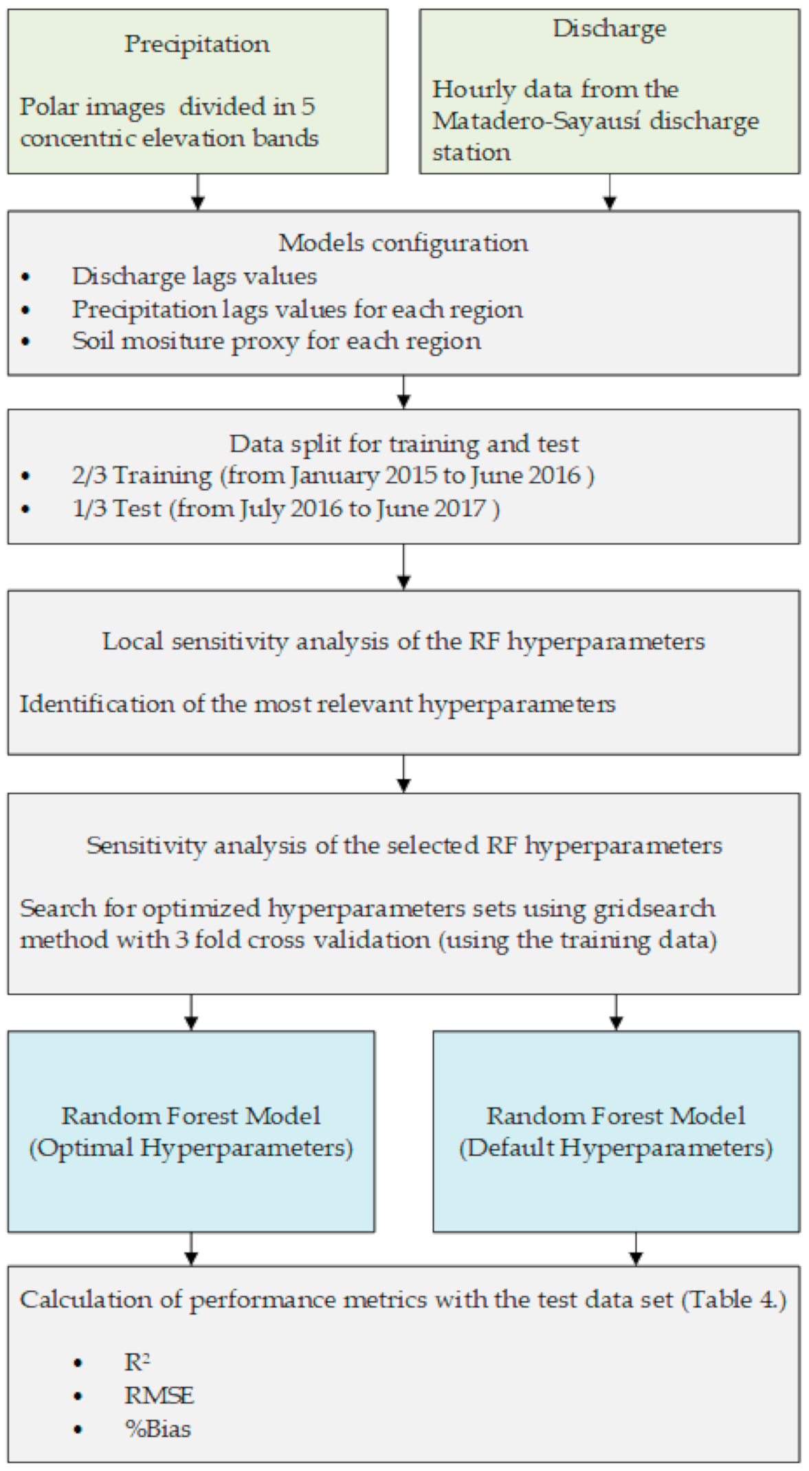
The main steps of the methodology of this study are depicted in the flowchart of Figure 2. At first, predictors for each runoff forecasting model (4-, 12-, and 24-h) were selected from the available data, i.e., precipitation and runoff time series (Section 2.4). Then, data were split for training-validation and test. The former was used for performing the sensitivity analysis of the RF hyperparameters. First, a local sensitivity analysis was used to identify the most relevant hyperparameters to be explored in detail. Afterwards, the grid search methodology was applied allowing to find optimized hyperparameter sets, which were ranked according to several performance metrics (Section 2.5). Finally, performance of the models set-up with all default hyper parameters vs. those that used an optimized hyperparameter sets were compared on the test dataset (Section 2.6).

2.4. Models Configuration

We built three RF runoff models, one for each forecasting lead time of 4, 12, and 24 h. For the configuration of each model, a key aspect is to define the input dataset (model features) from the available hourly time series of runoff and radar-based precipitation. For hydrological forecasting models, data from previous time steps (rainfall and runoff) also provide relevant information for improving the quality of the forecasts. For this reason, the model input features in this case corresponded to (i) previous records of instantaneous precipitation, (ii) previous records of instantaneous runoff, and (iii) accumulated precipitation values from the last 3 days, which represented a proxy variable for the soil moisture state. On the other hand, the target variable was the corresponding runoff value according to the forecast horizon.

To determine the number of lags of these variables, statistical analyses were conducted. For runoff, we relied on the partial- and auto-correlation functions by means of the correlogram with a 95% confidence band [37]. The confidence intervals were returned where the standard deviation was computed according to Bartlett’s equation and $\frac{1}{\sqrt{n}}$ (for $n$ observations), for autocorrelation and partial autocorrelation functions respectively [38]. For precipitation, we determined the number of lags to be used according to the Pearson correlation between the runoff time series and the precipitation time series of each elevation range. For this, we moved the latter 1 h backwards each time, to determine which lag is still representative according to the correlation value [19].

2.5. Sensitivity Analysis of Hyperparameters

We divided the sensitivity analyses of hyperparameters into two steps (Figure 2). First we performed a local sensitivity analysis in order to identify the most relevant hyperparameters that need further inspection. Here, a base model was first created by leaving all hyperparameters as their default values. Afterwards, vectors of possible values were defined for each hyperparameter to be analyzed (see

Table 2. Range of values for each hyperparameter used for the grid search method.

Hyperparameter	Value Vector; Increment
criterion	[mean absolute error, mean squared error]
max_depth	[5–70;5]
max_features	[6–48;6]
max_leaf_nodes	[5–50;5]
max_samples	[0.1–1;0.1]
min_samples_leaf	[1–20;5]
min_samples_split	[2, 5–40;5]
n_estimators	[10–100;10, 100–1000;100]

). Finally, new models (i.e., combination of hyperparameters) were built by varying one hyperparameter at the time and their performance were evaluated through the R² metric. Thus, we selected the hyperparameters that highly varied from their default value when reaching the highest model performances. This allowed us to identify the most relevant hyperparameters that needed a more detailed inspection.

Secondly, to better explore the influence of the selected most relevant hyperparameters, we used an approach that allows from a base model, to optimize its performance by adjusting its hyperparameters. There are several methods to explore and determine the optimal values for the hyperparameters such as randomized search, Bayesian optimization, and grid search, with the latter one being of the most widely employed [31,33]. We used the grid search methodology, which is an exhaustive search method where each hyperparameter under analysis is assigned to a vector of possible values. The method internally performs a K-fold Cross Validation (CV) process, which divides the training-validation data into K folds. For each iteration, one of the folds is isolated for validating, whereas the remaining k − 1 folds are used for training the data. Therefore, each fold was used exactly once as validation data. At the end, the results were averaged, and a single estimate of model performance was obtained.

This process was performed for all possible combinations between hyperparameter values (i.e., all possibilities in the range of those hyperparameters selected in the first step while all no-relevant hyperparameters were set to their default values) and returned the combination of hyperparameters that obtained the best performance according to R² metric calculated between observed and simulated data [39]. As this is an exhaustive search method, it was necessary to ensure that the optimal values of the hyperparameters were within the defined vectors [39]. An approach of 3-fold cross-validation was used in this study, which is a standard for evaluating the error in RF models.

We inspected the grid search results focusing on a sensitivity analyses. Thus, we used the results of the models that were built up with hyperparameter combinations where all except one of the hyperparameters were fixed to their optimized values while the remaining relevant hyperparameter varies through its domain (defined in the search feature space). This allowed inspecting the model performance evolution under a sensitivity analysis.

The analysis described was performed for the models built for different lead times: 4, 12, and 24 h. Afterwards, the impact of the hyperparameters for each lead time was analyzed in order to identify if the impact was consistent along all models at different forecast horizons.

2.6. Performance Evaluation Criteria

Three error metrics were used to evaluate the performance of the models: The coefficient of determination (R²), the root mean square error (RMSE), and percentage bias (%Bias) according to equations 1, 2, and 3, respectively.

$${\mathrm{R}}^2=1-\frac{S{S}_{error}}{S{S}_{total}}$$

(1)

where $S{S}_{error}$ is the sum of squares of the residuals, and $S{S}_{total}$ is the sum of the squares of the deviations of each observed value from the mean of the observations.

$$RMSE=\sqrt{\frac{{{\displaystyle \sum }}_{i=1}^n{\left(X_{obs,i}-X_{sim,i}\right)}^2}{n}}$$

(2)

$$\%Bias=100\ast \frac{{{\displaystyle \sum }}_{i=1}^n\left(X_{sim,i}-X_{obs,i}\right)}{{{\displaystyle \sum }}_{i=1}^n{X}_{obs,i}}$$

(3)

where $X_{obs,i}$ is the observed value and $X_{sim,i}$ is the simulated value at the time $i$.

3. Results

3.1. Models Configuration: Inputs Setup

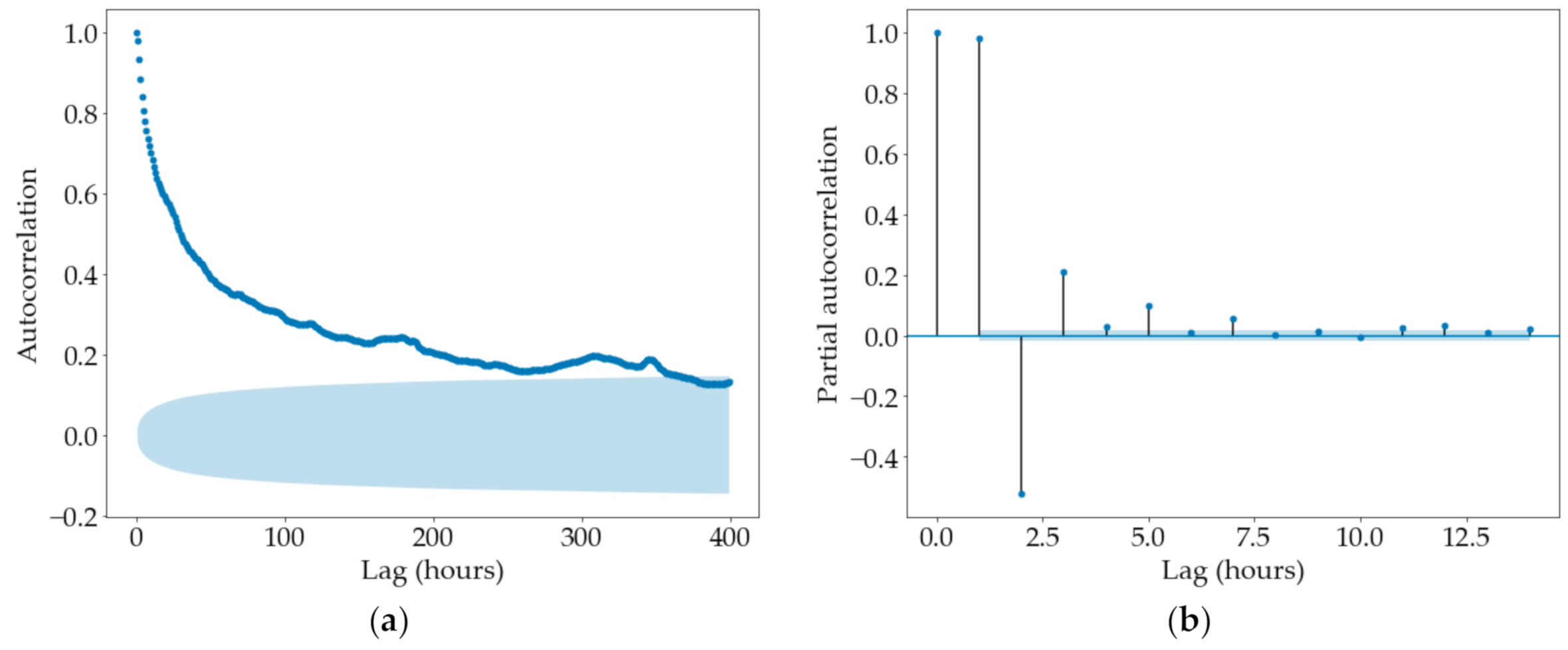
Figure 3 shows the plots of the partial- and auto-correlation functions together with their corresponding 95% confidence interval used for defining the number of runoff lags for the forecasting models. Figure 3a plots the autocorrelation function (ACF) calculated from lag 1 up to 400 (hours). We found a relatively high correlation (>0.25) up to approximately lag 100. However, correlations are significant up to lag 360, and thereafter, the correlation fell within the confidence band. The systematic ACF decay revealed a dominant autoregressive process. On the other hand, Figure 3b plots the partial autocorrelation function (PACF), which reveals a significant correlation up to lag 8, which then vanishes to null values (within the confidence interval). The rapid decay of the PACF indicates a dominance of the autoregressive over the moving-average process Therefore, we decided to use 8 runoff lags (hours) as predictors for the models.

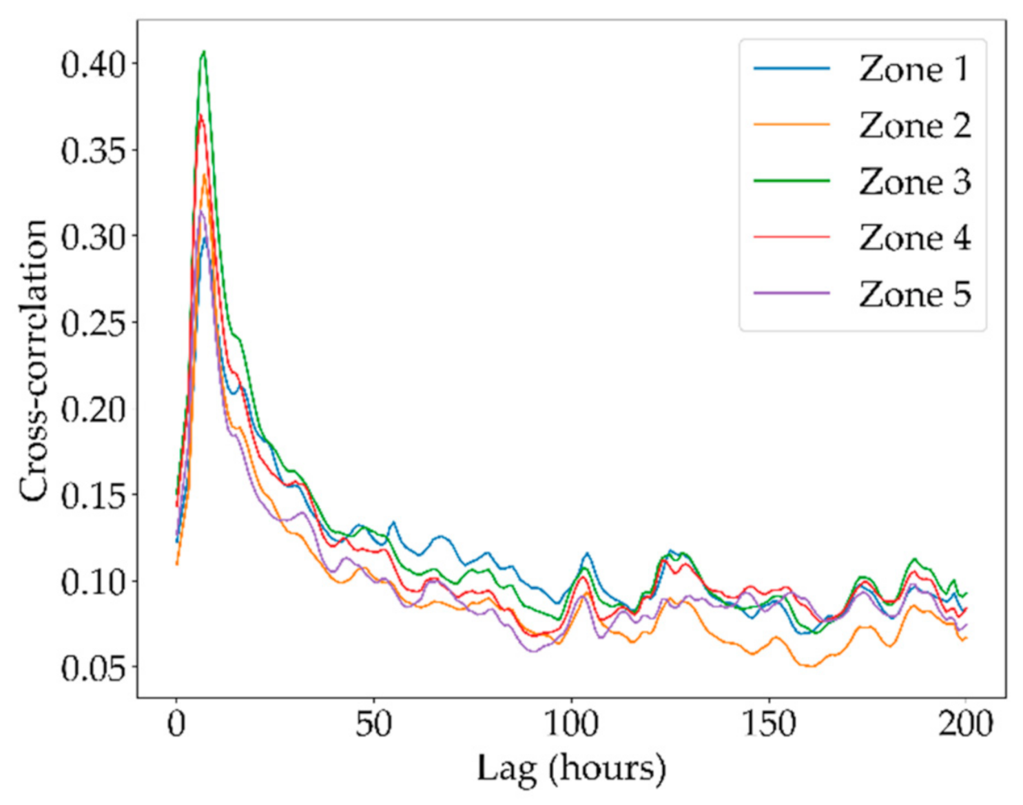
Moreover, we relied on the Pearson’s correlation between the runoff and precipitation timeseries for determining the number of precipitation lags to be used in the forecasting models. Results revealed maximum correlations, for all regions, at lag 8 (0.30, 0.34, 0.41, 0.37, 0.31), as depicted in Figure 4.

3.2. Sensitivity Analysis of Hyperparameters

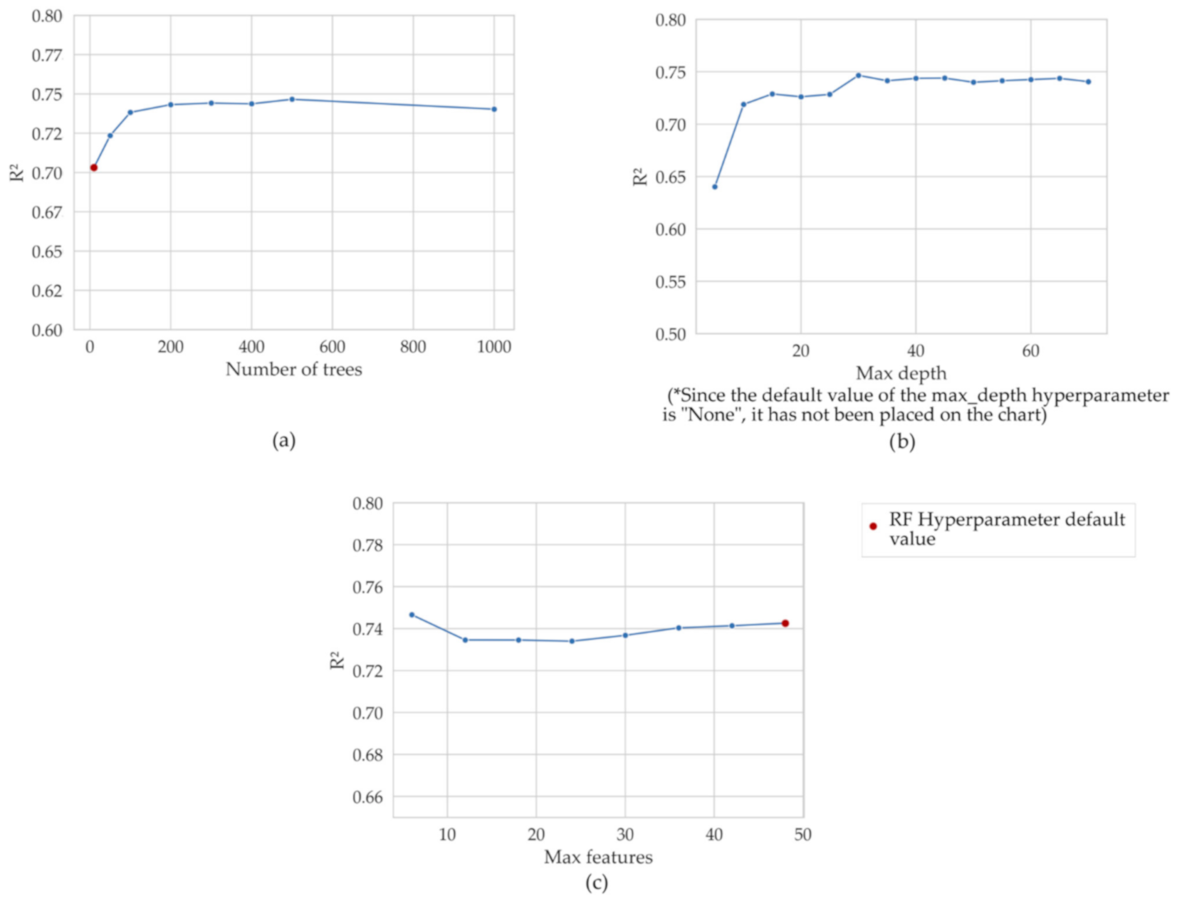
After performing the local sensitivity analysis, the hyperparameters that presented greater variability in their values when reaching high R² correspond to the maximum number of features (max_features: inputs to the model), the number of estimators (n_estimators: number of trees in the forest) and the maximum depth of the tree (max_depth: consecutive splits of a tree). Therefore, the subsequent analyzes were carried out only with these hyperparameters.

As a result of applying the grid search method with the selected hyperparameters, the optimal set of hyperparameters was obtained as well as the performance metric R² for each of the possible combinations. Figure 5 illustrates the evolution of the selected hyperparameters through the search space. Figure 5a,b depicts similar behaviors of the max_depth and n_estimators, where model efficiencies increase until reaching their maximum values. Thereafter, model performances remain almost constant (maximum variation of 0.03 for R²).

On the contrary, the n_estimators hyperparameter produced a variable efficiency behavior for small values (between 10 and 100), and thus generated a greater variability (0.04 for R²) when compared to the remaining hyperparameters However, after a threshold value is achieved (100 trees for the 12-h model), their efficiencies stabilized with a maximum variability of 0.01 for the training-validation subset.

The max_depth hyperparameter did not cause a significant variation in model performances. The variation in R² was less than 0.03 for the models with max_depth values along the range of 10–70. The hyperparameter max_features presented the best performance (R² = 0.75) for a relatively low number of features (6). The model performance decreased until R² = 0.73 for 24 number of features, then increased again slightly for the value of the max_features = 30 and continued to increase slightly for higher values (less than 0.01). Thus the performance was relatively stable for the entire range of values analyzed.

When analyzing the interrelation of the hyperparameters it was seen that for both hyperparameters, the number of trees, and the maximum depth, the model performance stabilizes after reaching a certain value (in this case, 100 and 15, respectively), and after that there were no significant improvements.

We found that best results were achieved when the three analyzed hyperparameters were in an optimal range. Moreover, although there was a combination of hyperparameters that cause the maximum performance of the model (0.75), there were many combinations of hyperparameters that caused a performance that was very close to the optimal one (above 0.74). Therefore, we can argue that certain ranges of values of the hyperparameters can reach a model performance close to the optimum. For example, for the hyperparameter n_estimators (number of trees), its range covered values greater than 50. In the case of the hyperparameter max_features, it presented results close to the optimal with both large and small values, the values with which the best results were obtained are 6, 36, 42, and 48. Furthermore, in the case of the max_depth hyperparameter, the best results were obtained when its value was 15 or higher.

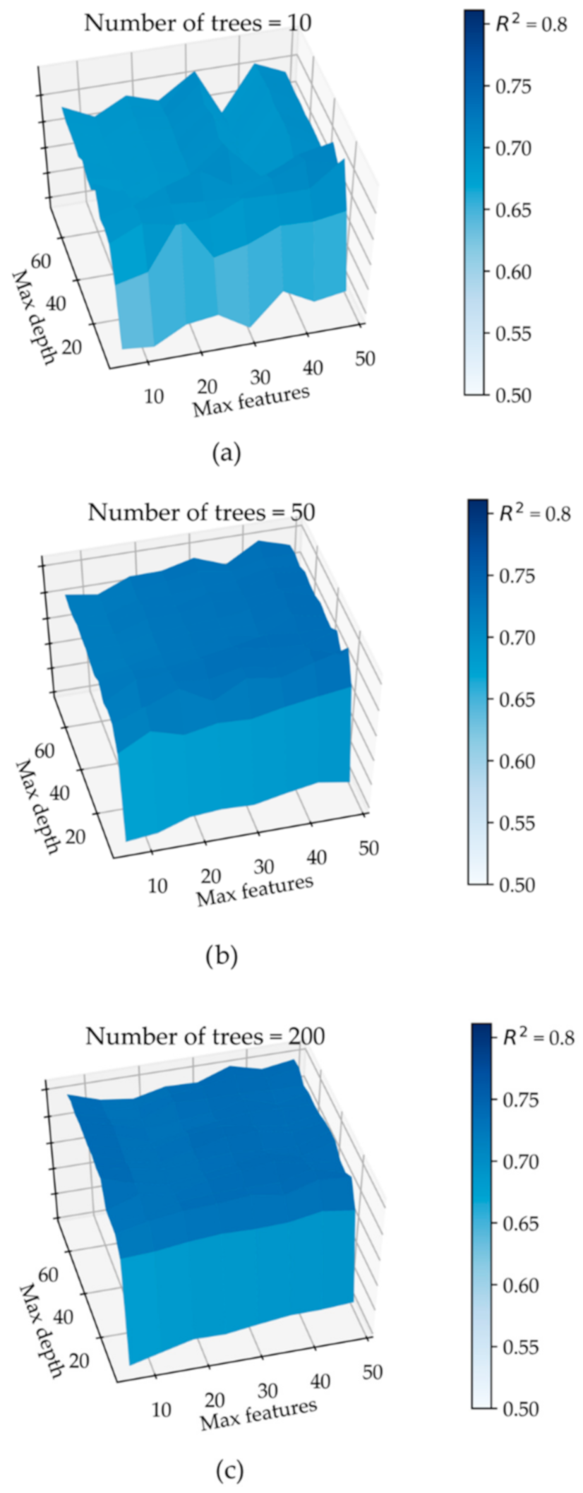
If any of the hyperparameter values were outside of its optimal range, it negatively affects the performance of the model. This can be seen in Figure 6, where we observed that when we set the value of the hyperparameter n_estimators in a non-optimal value such as 10 (Figure 6a), the performance did not exceed the value of 0.71, while when we set the value of this hyperparameter within the optimal range as 200 (Figure 6c) the performance reached up to 0.74.

3.3. Optimization of Hyperparameters at Different Lead Times

The next step was to compare the performance of the models built with default hyperparameters as well as optimal hyperparameters, for each lead time.

Table 3. Performance of the 4-, 12-, and 24-h runoff Random Forest (RF) models by using default hyperparameters and the test dataset.

Lead Time (Hours)	Training-Validation	Test
	R2	RMSE	%BIAS	R2
4	0.75	6.14	9.88	0.70
12	0.68	9.36	31.22	0.24
24	0.48	9.85	28.15	0.16

shows the performance of the models trained and tested using hyperparameter default values for each lead time. The main default values of the scikit-learn Python library are [36]: n_estimators = 10, max_features = total number of variables, max_depth = none). The performance of the default-value models was the benchmark against which we evaluated the models that used the set of optimized hyperparameters. Table 3 shows the efficiencies of the base models for the training-validation and test subsets. The latter corresponds to the entire independent set of data that were separated at the beginning of the process and was not used during the training-validation process.

Table 4. Optimal combination of RF hyperparameters for the 4-, 12- and 24-h runoff models and their corresponding performances.

Lead Time (Hours)	Optimal Hyperparameters			Training-Validation	Test
	n_estimators	max_features	max_depth	R2	RMSE	%BIAS	R2
4	500	42	30	0.85	5.96	10.12	0.69
12	500	6	30	0.75	8.26	24.33	0.41
24	500	6	35	0.54	9.01	29.02	0.29

shows the optimal set of hyperparameters, found when applying the grid search method, together with their corresponding model performances for the training-validation and test subsets.

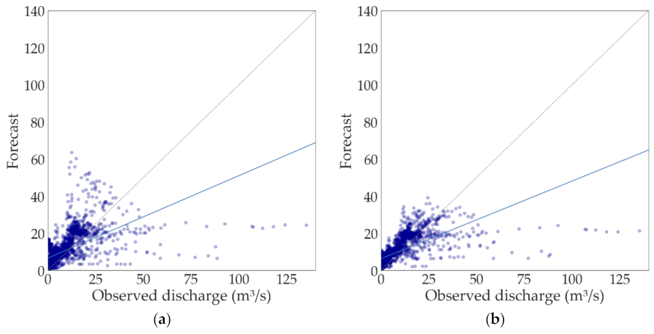
For all lead times, the models with optimized hyperparameters outperformed their corresponding base models, those with default hyperparameters. Performance improvements (R²) were 0.02, 0.16, and 0.14 for lead times of 4, 12, and 24 h, respectively. For instance, Figure 7 illustrates the scatter plot between the 12-h observed and predicted runoff using (a) default hyperparameters and (b) optimized hyperparameters. Results revealed the ability of the model to forecast runoffs up to 30 m³/s (20-year exceedance probability of less than 5%). Conversely, it seems clear the difficulty of the model to forecast extreme peak runoffs since a better representation of soil moisture may be required for modelling.

4. Discussion

The current study demonstrates, the improvement in the performance of the RF forecasting models by optimizing its hyperparameters for all lead times. We found that the optimal values were quite different from their default settings. The benefit of the models tuning became more significant for the forecasting models of 12 and 24 h.

The hyperparameters influence on models efficiencies could be explained by the generalization power of the RF algorithm, which, is driven by hydrological processes in this application. For runoff, a limiting concept in the development of forecasting models is the so-called concentration time of the catchment, which describes how fast the catchment responds to rainfall events. For the Tomebamba catchment, the concentration time is calculated between 4 to 6 h, and as the lead time exceeds this value, input data at short time intervals provides less information relevant for the forecasting. As a result, model optimization tends to rely more on the hyperparameterization than in what they can learn from the input data. This premise corroborates the findings of Huang and Boutros (2016) with respect to the influence of RF hyperparameters for datasets with reduced relevant feature spaces.

Consequently, as the lead time increases, more specific trees from the forest are required for reaching optimal model efficiencies. Here, the trees for the 4- and 12-h models (max_depth = 30) remained less specialized than the ones for the 24-h model. This is because the 4- and 12-h models possessed input features that better described the response of the catchment to rainfall events. Conversely, the 24-h model needs to rely on more specific trees and thus deeper trees with longer paths from root to leaf nodes (i.e., max_depth = 35).

Moreover, the benefit obtained by optimizing the max_features hyperparameter was also reported by Bernard et al. (2009) and [31] yet in other fields of research (dataset characteristics). We obtained the highest max_features value for the 4-h forecasting model. In other words, stronger randomization was required for the models of 12- and 24-h, which supports the hyperparameter influence on model efficiencies for longer lead times.

Among the analyzed hyperparameters, n_estimators showed the highest influence on the overall models performance, particularly along the range 0 < n_estimators < 100, where we found major improvements. This finding on the convergence behavior of model performance with n_estimators is consistent with that of Probst et al., (2018). Thus, calibrating n_estimators is the straightforward way to achieve near-optimal model efficiencies. However, despite the great influence of the n_estimators definition, the combination of max_features and max_depth might also play an important role during optimization. This can be noted in Figure 6 where, non-optimal combinations of max_depth and max_features lead to sub-optimal solutions (depressions in the solution surface, which are more notorious for non-optimal values of n_estimators). Thus, to ensure optimal model efficiencies, the three analyzed hyperparameters must be in their optimal range. Based on our results, we suggest, as a rule of thumb, to employ more than 100 trees for the n_estimators hyperparameter, and to focus on the combined hyperparameterization of max_depth and max_features. This suggestion complements the findings of Probst and Boulesteix (2017) who theoretically demonstrated that more trees are always better.

An added value of this study is to have for the very first time conducted a detailed sensitivity analysis of the most-influent RF hyperparameters for runoff forecasting applications. This is particularly important since most of the sensitivity analyses in data-driven runoff forecasting are focused on the inputs of the model rather than its hyperparameters. However, in ML-based models, hyperparametization can have a tremendous impact on the improvement of the model, which is usually overlooked. We did not assess the sensitivity occasioned by the input data but rather followed a specific methodology aimed to define the composition of the input data for each lead time. Therefore, our results are the combined effect of both the composition of the input data and the lead time. As a result, different input compositions might lead to different model hyperparameterization scenarios for each lead time. Thus, caution should be taken when interpreting the results of this study.

5. Conclusions

This study evaluated the impact of the most relevant RF hyperparameters (number of trees, maximum number of features, and maximum depth) in the performance of short-term runoff forecasting models in mountainous regions. By evaluating different forecast horizons it was possible to determine whether the impact was related to the lead time of forecasting. From the results, several conclusions were drawn:

(i)

Runoff forecasting model performance at 4 h denoted no significant difference in the R² metric by using both default and optimized hyperparameters. This is due to the relatively short lead-time forecasting that makes the input features become more relevant for the model. Therefore, even without performing a hyperparameter optimization process, a relatively high performance is obtained. On the other hand, for higher lead times (12- and 24-h) model performance is drastically improved when using optimized hyperparameters since they contribute more to the generalization of the model.

(ii)

The importance of RF hyperparameterization was demonstrated in this study (high variability of solution surfaces). Thus, we suggest performing sensitivity analyses on input composition as well as on the most relevant RF hyperparameters for achieving optimal runoff forecasting efficiencies. This is especially true for lead times exceeding the concentration time of the associated catchment.

(iii)

The hyperparameter that causes the greater improvement in model performance when applying the optimization is the number of trees. Default value of n_estimators = 10 produced poor results. However, when its value increased to 100 and forward, model performance increase dramatically, especially in high lead times (12, 24). Thus, for a straightforward improvement in the performance of runoff RF models we recommended setting the n_estimators hyperparameter higher to 100.

(iv)

The hyperparameter max_depth produced the highest variability-instability on the models. Although its impact also depends on the combination with the max_features hyperparameter, it seems that the depth of the tree plays a key role on the generalization capability of the models. This is obvious when considering that it allows the model to generate specific solutions. However, finding that several combinations of max_features only produce slight variations in the model performance allows the modeler to focus on finding an optimal solution for max_depth only. This will reduce the computing times in the training-validation phase and would allow for a deeper exploration regarding the input features.

In summary, several insights about the interaction of RF hyperparameters on runoff applications has been provided for the very first time. This has demonstrated the benefits of obtaining an optimized set of hyperparameters and highlighted some strategies when dealing with the optimization process. Further work will focus on the exploration of the influence of the hyperparameters under different sets of input features for every runoff forecasting model.