Uncertainty of Rate of Change in Korean Future Rainfall Extremes Using Non-Stationary GEV Model

Abstract

Interest in future rainfall extremes is increasing, but the lack of consistency in the future rainfall extremes outputs simulated in climate models increases the difficulty of establishing climate change adaptation measures for floods. In this study, a methodology is proposed to investigate future rainfall extremes using future surface air temperature (SAT) or dew point temperature (DPT). The non-stationarity of rainfall extremes is reflected through non-stationary frequency analysis using SAT or DPT as a co-variate. Among the parameters of generalized extreme value (GEV) distribution, the scale parameter is applied as a function of co-variate. Future daily rainfall extremes are projected from 16 future SAT and DPT ensembles obtained from two global climate models, four regional climate models, and two representative concentration pathway climate change scenarios. Compared with using only future rainfall data, it turns out that the proposed method using future temperature data can reduce the uncertainty of future rainfall extremes outputs if the value of the reference co-variate is properly set. In addition, the confidence interval of the rate of change of future rainfall extremes is quantified using the posterior distribution of the parameters of the GEV distribution sampled using Bayesian inference.

1. Introduction

In most studies investigating future rainfall extremes, it is assumed that future rainfall data simulated from global climate models (GCMs) or regional climate models (RCMs) are “observed” data in the future [1,2]. However, even recently developed climate models simulate temperature stably [3,4,5] but still expose many limitations to the simulation of rainfall extremes [6,7,8,9,10]. As can be found in the results of Kim et al. [11], very different future projection outputs are obtained depending on which RCM-simulated future rainfall data are used to analyze rainfall extremes. Recently, a series of attempts have been made to investigate future rainfall extremes based on the relationship between temperature and rainfall extremes [12,13,14]. The basic concept commonly included in these attempts is based on the fact that investigating the behavior of rainfall extremes under global warming conditions from the relationship between observed temperature and observed rainfall extremes is an approach to obtain more consistent future outputs [15,16].

In general, frequency analysis is often used to quantify rainfall extremes. The same goes for the quantification of future rainfall extremes. Hosseinzadehtalaei et al. [17] estimated rainfall quantiles from a stationary frequency analysis using the rainfall projection output for the 30 years from 2071 to 2100. They also estimated rainfall quantiles from another stationary frequency analysis using the present-period rainfall simulation output for 30 years from 1971 to 2000. Then, the rate of change of future rainfall extremes was estimated from the estimated rainfall quantiles for different periods. Stationary assumptions for segmented future periods can be found in many studies on rainfall extremes related to climate change [18,19,20]. In addition, studies on non-stationary frequency analysis have been actively conducted. The non-stationarity of time series of rainfall extremes is sometimes expressed explicitly as a function of time, but it can also be related to climate variables observed at the same time or the preceding time when rainfall extremes occurred [21]. According to several studies, it is reported that it is more reasonable to use climate variables than time as co-variates for expressing non-stationarity in a non-stationary frequency analysis [22,23]. Recently, studies of non-stationary frequency analysis using climate variables have been suggested for the annual maximum series [24,25,26,27,28,29,30,31,32]. However, studies that have produced practical projection outputs of rainfall extremes reflecting future climate information under future climate change scenarios using non-stationary frequency analysis are still lacking.

On the other hand, the issue of the validity of the non-stationary frequency analysis compared to the stationary frequency analysis has actually been a matter of much debate. Koutsoyiannis and Montanari [33] stated that after making past observations into a stationary process, i.e., after adjusting to represent future conditions, it was good to describe future conditions in the stationary domain. Serinaldi and Kilsby [34] warned that uncertainty might increase when the non-stationary model is applied since the non-stationary model is more complex than the stationary model. In addition, De Luca and Galasso [35] pointed out that, assuming that the process was non-stationary, ergodicity could not be maintained, so possible trends should be derived from an external source different from the time series of interest. Therefore, they argued that it was not essential to adopt a non-stationary model. On the other hand, studies showing that a co-variate-based non-stationary frequency analysis is more appropriate to convincingly project rainfall extremes in the future have also been actively proposed [10,12,15,31,36].

One of the important issues in the frequency analysis of rainfall extremes is how to evaluate the relative superiority of the stationary and non-stationary models. In general, the excellence of a model is discussed using the Akaike Information Criterion (AIC), which evaluates the fitness of the annual maximum series and probability distribution, or similar indicators [37,38]. However, the results of goodness of fit are very likely to vary depending on the sample size. From the other side, it can be said that the uncertainty of the quantiles derived from the results of a frequency analysis play an important role in discussing the excellence of the model [34]. The smaller the uncertainty of the estimated quantiles, the more reliable the model can be recognized as [39]. Ouarda et al. [36] pointed out that uncertainty is likely to act as a major weakness in the applicability of non-stationary models through stationary and non-stationary frequency analyses of annual maximum rainfall in the UAE. However, studies suggesting a methodology that can reduce uncertainty are still difficult to find.

In this work, a methodological study focused on a specific statistical approach was performed, and it is different from previous studies in the following three aspects. The first is that it discusses the results of deriving projection outputs of future rainfall extremes reflecting future climate information using a non-stationary frequency analysis. The second is that it introduces the concept of determination of the optimal model, focusing on the uncertainty as well as the fitness of the data, and the concept of a reference co-variate to reduce the uncertainty of the non-stationary frequency analysis. The third is that it investigates the uncertainty of future rainfall extremes by dividing the inter-model variability generated from various climate model combinations and the uncertainty of the co-variate-based non-stationary frequency analysis model, and it identifies the uncertainty of the rate of change of future rainfall extremes.

This study proceeds as follows: (1) A non-stationary frequency analysis of the annual maximum daily rainfall time series (AMR) using surface air temperature (SAT) or dew point temperature (DPT) as a co-variate is performed. (2) Using the Bayesian approach, parameters of the stationary and non-stationary generalized extreme value (GEV) distributions for the AMR are sampled from the posterior distribution. (3) Using this, we evaluate the performance of the stationary frequency analysis and the non-stationary frequency analysis in terms of uncertainty. (4) We investigate how uncertainty in the non-stationary frequency analysis can be reduced by determining the appropriate co-variate reference value corresponding to the rainfall quantile. (5) We present the rate of change in rainfall quantile under climate change scenario conditions using future information of SAT or DPT produced from a combination of various climate models. (6) The uncertainty of the rate of change of future rainfall extremes is analyzed using the information obtained from the non-stationary frequency analysis by the Bayesian approach.

2. Data and Methods

2.1. Data

We used the daily mean SAT, daily mean DPT, and daily precipitation of two Automated Surface Observing System (ASOS) meteorological observation sites (Chuncheon and Cheonan) operated by the Korea Meteorological Agency (KMA) [40]. The Chuncheon site is located in a mountainous area of the central part of the Korean Peninsula, and the Cheonan site is located in a plain area of the western part of the Korean Peninsula. The data period was from 1973 to 2019. Figure 1 shows the spatial location of the sites used.

The Coordinated Regional Climate Downscaling Experiment East-Asia (CORDEX-EA) team recently produced future climate information for the East Asian region from various GCMs and RCMs. There are two main types of future climate outputs developed by CORDEX-EA: 50-km spatial resolution outputs for East Asia and 12.5-km spatial resolution outputs for Korea. Future climate outputs with a spatial resolution of 12.5 km, produced from a total of 8 GCM–RCM combinations from 2 GCMs, including the Hadley Center Global Environment Model version 2-coupled Atmosphere-Ocean model (HadGEM2-AO, H2) and the Max Planck Institute Earth System Model—Low Resolution (MPI-ESM-LR, E6), and 4 RCMs, including the Fifth-Generation Penn State/NCAR Mesoscale Model (MM5), the Regional Spectral Model (RSM), RegCM4 (the latest version of the Regional Climate Model system), and the Weather Research and Forecasting model (WRF), were used in this study. In addition, Representative Concentration Pathway (RCP) 4.5 and RCP 8.5 were applied as future climate change scenarios. That is, a total of 16 future climate ensembles were used. For reference, the climate information outputs produced from a combination of climate modes consist of present data from 1981 to 2010 and future data from 2021 to 2050 [41]. The climate model outputs’ information is summarized in

Table 1. Climate model output information.

GCM	HadGEM2-AO (H2)				MPI-ESM-LR (E6)
RCM	MM5	RSM	RegCM4	WRF	MM5	RSM	RegCM4	WRF
Temporal resolution	3-h
Spatial resolution	12.5 km
Variables	Atmospheric pressure, maximum/minimum surface air temperature, specific humidity, precipitation
Scenarios	RCP 4.5/RCP 8.5
Temporal domain	Present: 1981–2010 Future: 2021–2050

. All data of daily outputs produced by the combination of climate models were applied after bias correction by the quantile mapping process [42] linked to the Boe method [43].

2.2. Non-Stationary GEV Distribution

In this study, GEV distribution was applied as a probability distribution for frequency analysis of the AMR. The probability density function $\mathrm{f}\left(\mathrm{x}\right)$ of the GEV distribution is as follows:

$$\mathrm{f}\left(\mathrm{x}\right)= \frac{1}{\alpha }{\left\{1-\frac{\beta \left(x-x_o\right)}{\alpha }\right\}}^{\frac{1}{\beta }-1}exp\left[-{\left\{1-\frac{\beta \left(x-x_o\right)}{\alpha }\right\}}^{1/\beta }\right],$$

(1)

where $\mathsf{\alpha }$ is the scale parameter, $\mathsf{\beta }$ is the shape parameter, and $x_o$ is the location parameter.

From Equation (1), one can calculate the quantile $x_T$ corresponding to the return level of $\mathrm{T}$-year in the GEV distribution as follows:

$$x_T=x_o+ \frac{\alpha }{\beta }{\left\{1-\left(-ln\left[1-\frac{1}{T}\right]\right)\right\}}^{\beta },$$

(2)

Traditionally, the GEV distribution assumes that observations are independent and identically distributed. However, in order to model non-stationarity in the AMR time series, many researchers allowed the parameters of the GEV distribution to change depending on the co-variate [10,22,27,28,29,31,32,36,39]. In theory, all parameters of the GEV distribution can be applied as a function of various co-variates, but in this study, a co-variate was applied only to the scale parameter alpha, as shown below, in order to intuitively understand the effect of the co-variate.

Non-stationary model $n_1$:

$$\alpha \left(y\right)=exp\left[{\alpha }_1+{\alpha }_{2}SAT\left(y\right)\right],$$

(3)

Non-stationary model $n_2$:

$$\alpha \left(y\right)=exp\left[{\alpha }_1+{\alpha }_{2}DPT\left(y\right)\right],$$

(4)

where $SAT\left(y\right)$ is the SAT observed on the day on which the AMR occurred in year $\mathrm{y}$, and $DPT\left(y\right)$ is the DPT observed on the day on which the AMR occurred in year $\mathrm{y}$.

Therefore, one can calculate the quantile $x_T$ corresponding to the return level of the $\mathrm{T}$-year of the non-stationary model as follows:

$$x_T\left(y\right)=x_o+ \frac{\alpha \left(y\right)}{\beta }{\left\{1-\left(-ln\left[1-\frac{1}{T}\right]\right)\right\}}^{\beta },$$

(5)

That is, the quantile corresponding to the return level of the $\mathrm{T}$-year of the non-stationary model has various values depending on the co-variate. Since the current hydraulic structure design practice is based on the fact that the quantile corresponding to the return level of the $\mathrm{T}$-year in the stationary model has a single value, the dependence of the quantile on the co-variate in non-stationary models acts as a major cause that makes practical application of non-stationary models difficult.

3. Results

3.1. Parameter Estimation and Uncertainty

The parameters of the GEV distribution were estimated using the Metropolis–Hastings (MH) algorithm.

Table 2. Parameters and negative log likelihood.

Site	Parameter	Stationary s	Non-Stationary n_1	Non-Stationary n_2
Chuncheon	alpha_1	47.1039	3.2278	3.3694
	alpha_2		0.0273	0.0224
	beta	−0.1498	−0.1081	−0.0956
	x_o	110.8374	111.3025	111.1759
	nllh	209.4338	209.2788	209.3763
Cheonan	alpha_1	35.6845	2.5806	2.7541
	alpha_2		0.0417	0.0363
	beta	−0.0948	−0.0624	−0.0492
	x_o	105.3882	104.6429	106.0307
	nllh	193.561	194.4651	192.0164

shows the parameters and negative log likelihood ($\mathrm{nllh}$) estimated by fitting each of the three models to the observed AMR. The bold numbers denote the model representing the smallest $\mathrm{nllh}$. The AMR of the Chuncheon site showed the best fit when applying the non-stationary model $n_1$ (i.e., using SAT as a co-variate of the scale parameter). The AMR of the Cheonan site showed the best fit when applying the non-stationary model $n_2$ (that is, using DPT as a co-variate of the scale parameter). However, the AIC (where AIC = 2 × (# of parameters) + 2 × nllh) reflecting the parsimony point of view recommends that it is more appropriate to apply the stationary model $\mathrm{s}$ for both AMRs of both sites. That is, as applied in Lee et al. [10] and Ouarda et al. [36], if an optimal model is selected using the AIC, which mainly considers the aspect of fitness of the observed AMR, the stationary model $\mathrm{s}$ is selected as the optimal model for the AMR at Chuncheon and Cheonan sites.

The fundamental purpose of performing a frequency analysis is to estimate the rainfall quantile. However, since the parameters of the probability distribution necessary for estimation of the quantile are estimated from limited samples, uncertainty is bound to be included in the parameter of the probability distribution and the corresponding rainfall quantile. Therefore, if the sample size changes (i.e., when new data become available or when sampling is performed through other techniques), the selection result of the optimal frequency analysis model centered on fitness with a limited sample such as AIC is likely to change. Our argument is that the uncertainty of the probability distribution parameter and rainfall quantile gives important information in selecting the optimal frequency analysis model. In other words, identifying in which model the uncertainty of the parameter and rainfall quantile is the lowest can be an important determinant in selecting an optimal model. This is based on the fact that a model with less uncertainty in the parameter and rainfall quantile can be recognized as a more reliable model. We quantified the uncertainty of the model as follows:

$$p-factor=\frac{Width of 95\mathrm{PPU} for parameter ensemble}{Parameter ensemble average},$$

(6)

$$q-factor=\frac{Width of 95\mathrm{PPU} for rainfall quantile ensemble}{Rainfall quantile ensemble average},$$

(7)

where $95\mathrm{PPU}$ (Percent Prediction Uncertainty) means the 95% confidence interval of the corresponding variable [44].

A total of 10,000 parameters were sampled from the posterior distribution of parameters using Markov chain Monte Carlo (MCMC), and 10,000 rainfall quantile ensembles corresponding to the return level of 50 years were simulated. Equations (6) and (7) were used to quantify the uncertainty about the parameter and the uncertainty about the rainfall quantile.

Table 3. Uncertainty of stationary and non-stationary frequency analysis.

Site	Factor	Parameter	Stationary s	Non-Stationary n_1	Non-Stationary n_2
Chuncheon	P	α1		0.4651	0.4886
		α2		2.6020	3.5664
		α	0.5465	0.5306	0.5219
		β	−2.6478	−3.1391	−2.9063
		xo	0.2736	0.2659	0.2516
	q	50-yr	0.8356	0.7329 (0.7003)	0.5952 (0.5572)
Cheonan	P	α1		0.9012	0.7639
		α2		2.4406	2.6169
		α	0.4782	0.4909	0.5527
		β	−2.9555	−5.5192	−5.2905
		xo	0.2037	0.2236	0.1876
	q	50-yr	0.5998	0.8057 0.7624	0.5978 (0.5706)

shows the results. The parameters of the stationary model $\mathrm{s}$ are $\mathsf{\alpha }$, $\mathsf{\beta }$, and $x_o$, while the parameters of the non-stationary models ($n_1$ and $n_2$) are ${\alpha }_1$, ${\alpha }_2$, $\mathsf{\beta }$, and $x_o$. For direct comparison between models, the p-factor converted from ${\alpha }_1$ and ${\alpha }_2$ of non-stationary models to $\mathsf{\alpha }$ is also expressed. The $\mathsf{\alpha }$ of the non-stationary model was calculated using $\exp \left[{\alpha }_1 + {\alpha }_2\mathrm{E}\left[\mathrm{SAT}\right]\right]$ or $\exp \left[{\alpha }_1 + {\alpha }_2\mathrm{E}\left[\mathrm{DPT}\right]\right]$. The $\mathrm{E}\left[\mathrm{SAT}\right]$ or $\mathrm{E}\left[\mathrm{DPT}\right]$ is the average of the SAT or DPT corresponding to each AMR, respectively. The bold numbers denote the parameter representing the smallest uncertainty.

If a reliable model is selected based on the uncertainty of parameters, it can be recognized that the optimal model for the AMR at the Chuncheon site is the non-stationary model $n_2$, and the optimal model for the AMR at the Cheonan site is the stationary model $\mathrm{s}$. For the AMR at the Chuncheon site, the p-factor of the scale parameter and the location parameter was the smallest in the non-stationary model $n_2$. For the AMR at the Cheonan site, the p-factors of the scale parameter and the shape parameter were the smallest in the stationary model $\mathrm{s}$. However, the p-factor of all parameters in the optimal model is not smaller than the p-factor of parameters in other candidate models. Selecting the optimal model based on the p-factor of parameters may involve a lot of subjectivity.

The q-factor of the rainfall quantile corresponding to the return level of 50 years was calculated in two ways. The first method was to calculate the q-factor using the rainfall quantile ensemble reflecting all observed co-variate values. The second method was to calculate the q-factor of the rainfall quantile ensemble under the condition of $\mathrm{E}\left[\mathrm{SAT}\right]$ or $\mathrm{E}\left[\mathrm{DPT}\right]$ (numbers in parentheses in Table 3). Since the q-factor by the first calculation method adds co-variate change to the uncertainty caused by parameter estimation, the q-factor from the first calculation method becomes larger than the q-factor of the second calculation method. This fact was also discussed in Ouarda et al. [37]. However, it can be found that the difference between the values of the q-factor calculated by the first method and the second method is not very large. This suggests that in the range of values of SAT or DPT observed routinely, the effect of the change in co-variate on the uncertainty of the rainfall quantile is limited.

If the optimal model is selected using the uncertainty of the rainfall quantile, that is, the q-factor, it can be recognized that the optimal model for AMR at both sites is the non-stationary model $n_2$.

Table 4. Results of determining optimal model.

Site	nllh	AIC	p-Factor	q-Factor
Chuncheon	n1	s	n2	n2
Cheonan	n2	s	s	n2

shows the results of selecting the optimal model using $\mathrm{nllh}$, AIC, p-factor, and q-factor. The penalty for the number of parameters in AIC is to evaluate the model by reflecting the uncertainty of the model. However, evaluating the model using the p-factor or q-factor is a more direct reflection of the uncertainty. As described above, since the optimal model for the p-factor may vary for each parameter, it is more preferable to use the q-factor rather than the p-factor to evaluate the reliability of the model. Our proposal is to evaluate the fitness of the model for AMR using $\mathrm{nllh}$ and the reliability of the model using the q-factor. Therefore, the optimal model for AMR at the Chuncheon site can be determined as the non-stationary model $n_1$ or $n_2$. Similarly, it can be said that the non-stationary model $n_2$ is recommended as the optimal model for AMR at the Cheonan site.

Figure 2 shows the response of the rainfall quantile to the change in co-variate and the probability distribution of the observed co-variate. The ensemble average of the rainfall quantile by model $\mathrm{s}$ represents a single value regardless of the co-variate, and the width of the 95% confidence interval is not related to the co-variate. However, it should be noted that the ensemble average and 95% confidence interval by models $n_1$ and $n_2$ respond to the values of the co-variates observed on the day of AMR. The range of the ensemble of rainfall quantiles by non-stationary models is likely to be wider than the range of the ensemble of rainfall quantiles by the stationary model since the co-variate change is additionally reflected in addition to parameter uncertainty. In other words, the uncertainty of the rainfall quantiles by non-stationary models needs to be recalculated by reflecting only the uncertainty due to parameters by designating an appropriate co-variate value. The question is how to specify the appropriate co-variate value.

We pay attention to Equations (2) and (5) to find the appropriate co-variate value, that is, the reference co-variate value. Equation (5) returns the rainfall quantile corresponding to the return level of the $\mathrm{T}$-year in the non-stationary GEV distribution. Equation (2) returns the rainfall quantile of the stationary GEV distribution. Equations (2) and (5) can be used to calculate the value of the reference co-variate of the non-stationary GEV distribution, which returns the same rainfall quantile as the stationary GEV distribution. Reference co-variates for various return levels of AMR at the Chuncheon site and the Cheonan site are shown in Figure 3. In this study, based on the observed AMR, a method of estimating reference co-variates corresponding to various return levels is proposed under the assumption that the rainfall quantiles for each return level of the stationary model and the non-stationary model are the same. However, the relationship between the reference co-variate and the return level is not yet clear. In addition, the uncertainty of the reference co-variate should be further revealed. Reference co-variates may be an important research topic in co-variate-based non-stationary frequency analysis in the future.

Although not covered in this study, the bivariate frequency analysis related to co-variates could be one of the important research topics. Although not related to co-variates, the studies of Shiau [45], which applied a bivariate extreme value distribution to model extreme floods for flood volumes and flood peaks, Serinaldi [46], which emphasized a clear understanding of the return level in non-stationary frequency analysis, and De Luca et al. [47], which evaluated the return level of a design hyetograph using the concept of copula, can be said to provide good insight in the context of future expansion of this topic.

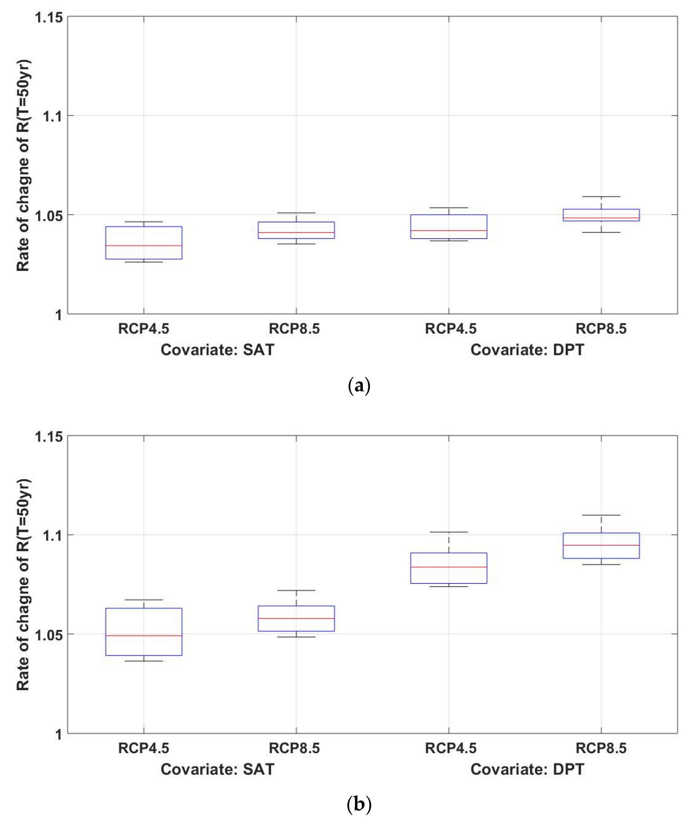
3.2. Future Rainfall Extremes

In most studies, including those of Hosseinzadehtalaei et al. [17] and Kim et al. [11], the future rainfall extremes taking into account climate change scenarios are estimated based on the ratio of rainfall quantiles under present climate conditions to rainfall quantiles under future climate conditions (i.e., rate of change). When estimating the rainfall quantile in present or future climate conditions, stationary conditions are generally assumed for each period (e.g., 1980–2010, 2021–2050, and 2071–2100). That is, the present rainfall quantile is estimated under the assumption that the AMR produced from the climate model under the present climate condition satisfies the stationary condition, and the future rainfall quantile is estimated under the assumption that the AMR produced under the future climate condition also satisfies another stationary condition. Figure 4a shows the results of projecting the rate of change of future rainfall extremes using this approach. The rate of change is defined as [future rainfall quantile]/[present rainfall quantile]. That is, a rate of change of 1.2 means that the future rainfall quantile will increase by 20% over the present rainfall quantile.

Based on the ensemble average of the rate of change by eight climate model combinations, the rainfall extremes in the future period (2021–2050) are likely to increase from 8% to 24% over the rainfall extremes in the present period (1981–2010). However, depending on which climate model combination is applied, the rate of change has very different values (0.67–1.81). It can even be found that cases where the rate of change is greater than 1 (i.e., rainfall extremes increase) and less than 1 (i.e., rainfall extremes decrease) are occurring simultaneously. Figure 4b,c show the rate of change in annual average SAT and DPT. Compared with rainfall extremes, it can be seen that the fluctuation range of the rate of change for each combination of climate models is significantly reduced. In addition, regardless of the combination of climate models applied, the rate of change shows a consistent increase pattern. These results, coupled with the results of Section 3.1 which state that temperature is the recommended co-variate for the estimation of rainfall extremes, can be said to suggest a new approach to producing more reliable future rainfall extremes outputs.

A trend analysis of SAT and DPT produced from various climate model combinations was performed to estimate future rainfall extremes reflecting climate change scenarios from co-variate-based non-stationary models derived from observations described in Section 3.1. The trend was assumed to be linear, as shown in Equations (8) or (9). The yearly SAT and DPT calculated from the daily SAT and DPT time series for the present and future periods produced for each climate model combination were used for the linear trend analysis.

$$\mathsf{\Delta }SA{T}_Y={\beta }_s\left(Y-2010\right),$$

(8)

$$\mathsf{\Delta }DP{T}_Y={\beta }_d\left(Y-2010\right),$$

(9)

where $Y$ is the future year, and $\mathsf{\Delta }SA{T}_Y$ and $\mathsf{\Delta }DP{T}_Y$ are the annual mean SAT or DPT at future year $Y$ minus the average of SAT or DPT for the present period (1981–2010), respectively. In Equations (8) and (9), 2010 means the last year of the present period.

From the trend analysis of SAT and DPT, one can set the scale parameter of the GEV distribution for a specific year in the future as follows:

Non-stationary model $n_1$:

$$\alpha \left(y\right)=exp\left[{\alpha }_1+{\alpha }_2\left(SA{T}_r+\mathsf{\Delta }SA{T}_Y\right)\right],$$

(10)

Non-stationary model $n_2$:

$$\alpha \left(y\right)=exp\left[{\alpha }_1+{\alpha }_2\left(DP{T}_r+\mathsf{\Delta }DP{T}_Y\right)\right],$$

(11)

where $SA{T}_r$ and $DP{T}_r$ are the reference SAT and DPT for the return level obtained in Figure 3, respectively. Figure 5 shows the time evolution of the scale parameter of model $n_2$ at the Cheonan site. It can be found that the scale parameter increases gradually in the future.

4. Discussion and Application

4.1. Decision Making from Ensemble Average and Uncertainty

How to reflect the impact of climate change in the estimation of the design rainfall depth is a task in the new normal era facing hydrologists. The most common way to investigate changes in future rainfall extremes is to use future rainfall data derived from climate models with climate change scenarios applied. In the early days, future rainfall extremes were estimated using rainfall data predicted from one climate model [19], but it has been established that it is desirable to use ensembles simulated in various climate models [20]. To quantify uncertainty in future climate change with a probabilistic approach, an ensemble of various climate model combinations is needed [1]. The reason why many researchers use the ensemble approach and try to obtain a better ensemble is to determine what the rate of change of future rainfall extremes will be in the end. In terms of climate change adaptation policy, the rate of change of the design rainfall depth at a specific duration for a specific return level at a specific site should eventually be given as a single value. This single value will be the ensemble average no matter what method we take [2,11]. However, as shown in previous studies [10,17] and Figure 4a of this study, the future rainfall extremes estimated by the stationary frequency analysis method using future rainfall data showed a lot of variation depending on which climate model combination was applied. In other words, the inter-model variability was very high. Even the future rainfall extremes of a specific site tend to increase in some combinations of climate models and decrease in other combinations of climate models. If the deviation between the ensemble members constituting the ensemble average is too large (i.e., the uncertainty is too large), policy decisions based on the ensemble average struggle to obtain credibility from the general public [15]. In fact, the large inter-model variability of future rainfall extremes has been proven through many studies [6,7]. Therefore, the reliability of future rainfall extremes projection at a specific site is generally low. Therefore, we need a new approach that can convince the general public about the uncertain future rainfall extremes.

We thought that a new approach to presenting convincing future rainfall extremes to the general public is to reduce the gap between future ensemble members. From the perspective of reducing the differences arising from various climate model combinations, the comparison of the results of Figure 4a and Figure 6 suggests that using future SAT or DPT in conjunction with a non-stationary model is better than using future AMR values. Consistency of future projections will contribute to future rainfall extremes gaining public trust and being reflected in policy.

The total uncertainty of future rainfall extremes decomposed into major sources is plotted in Figure 7. The total uncertainty was expressed as the coefficient of variation of samples extracted from the posterior distribution of future rainfall extremes. When the stationary model was applied, the uncertainty due to parameter estimation and the uncertainty due to various climate model combinations were similar. In fact, the uncertainty resulting from the estimation of the parameter of probability distribution is directly related to the data period we have observed. It is very difficult to reduce the uncertainty arising from parameter estimation since it is actually difficult to artificially increase the data period. The uncertainty of these two sources, parameter estimates and climate model combinations, can be found to propagate, without loss, to estimates of future rainfall quantiles. On the other hand, it can be found that most of the uncertainty included in the future rainfall quantile estimated from the co-variate-based non-stationary model is due to the parameter estimation of the GEV distribution. This result is because various combinations of climate models simulate similar future SATs or DPTs. In other words, this means that even if an ensemble of various climate model combinations is applied, the uncertainty of rainfall extremes does not increase significantly.

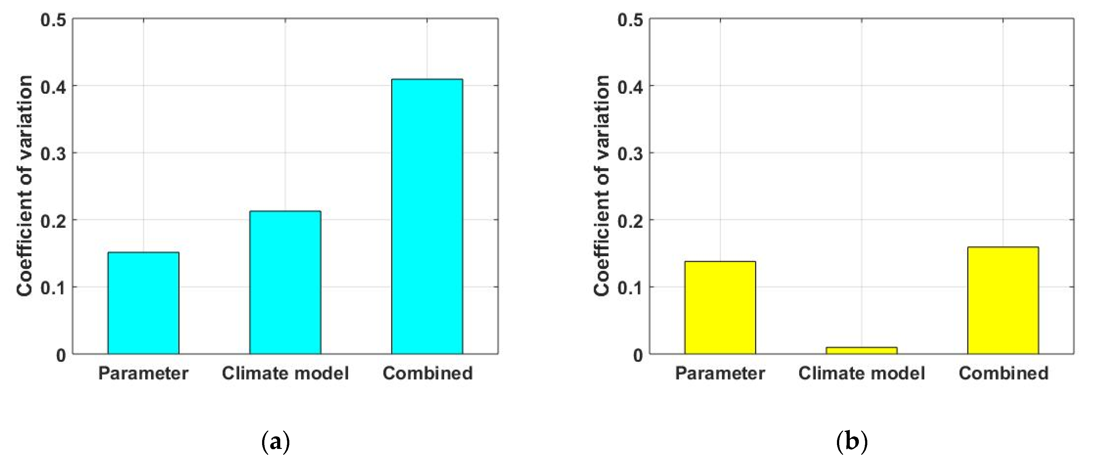
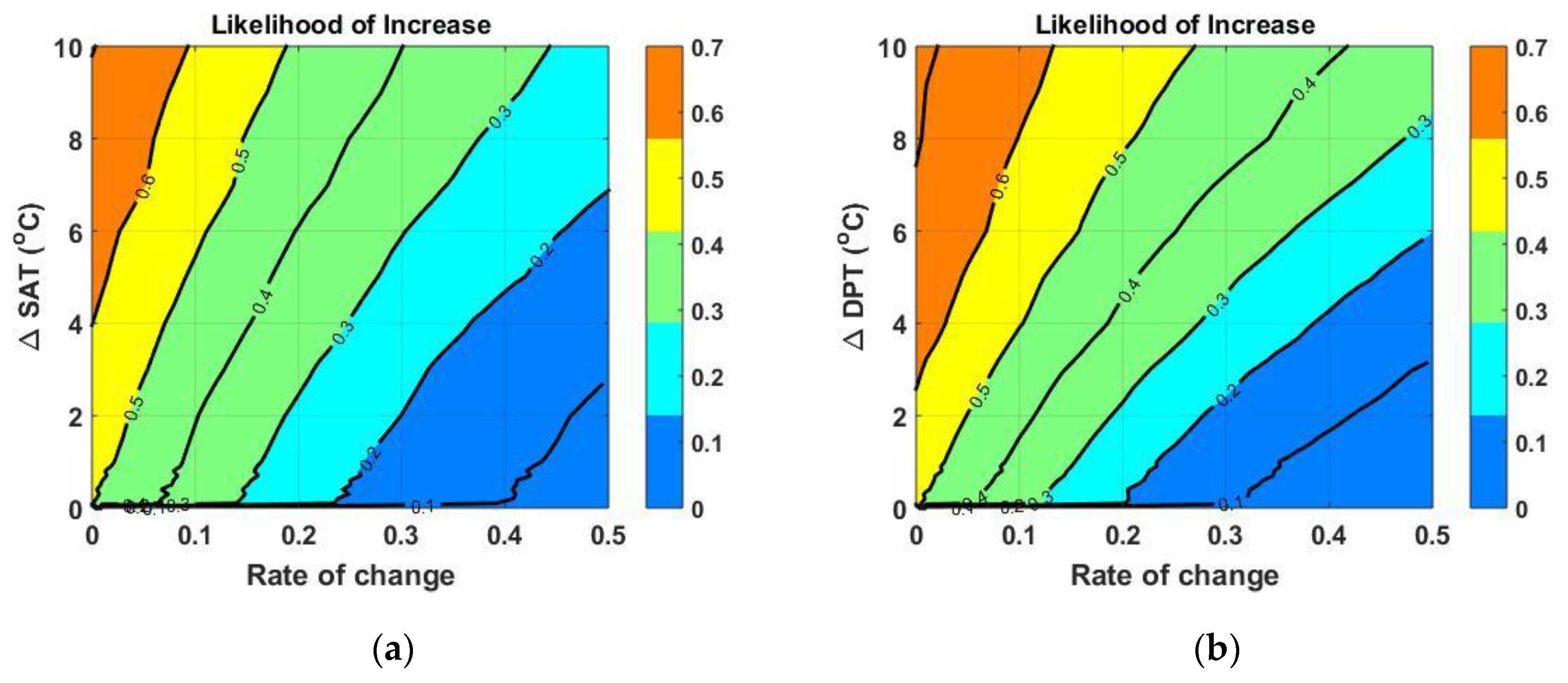
4.2. Uncertainty of Rate of Change

In this section, as an application of the proposed approach, we tried to quantify the rate of change of rainfall extremes for future temperature increase and the degree of uncertainty in such a rate of change.

By combining the non-stationary model $n_1$ and Equation (10) or the non-stationary model $n_2$ and Equation (11), an ensemble of rainfall quantiles corresponding to the increase in SAT or DPT can be obtained. Figure 8 shows the probability that the rainfall quantile for the return level of 50 years exceeds a certain rate of change (i.e., likelihood of increase, LoI) given that SAT or DPT increase ($\Delta \mathrm{SAT}$ or $\Delta \mathrm{DPT}$). For example, in the scenario in which the SAT rises by 6 °C at the Chuncheon site, the probability that the rainfall quantile for the 50-year return level increases by 20% or more is about 40%. Similarly, in the scenario where the DPT rises by 4 °C at the Cheonan site, it can be found that the probability of a rate of change of 1.1 or higher is about 50%.

If Figure 8 is substituted for a specific DPT rise scenario, the cumulative probability distribution for the rate of change of the rainfall quantile can be obtained as follows. The $\mathrm{LoI}\left(\mathrm{r}\right)$ in Figure 8 is the probability that the rate of change of the rainfall quantile for a specific return level is more than $\mathrm{r}$ under a specific DPT rising condition, so the probability that the rate of change is less than $\mathrm{r}$ is $1-\mathrm{LoI}\left(\mathrm{r}\right)$. That is, the cumulative probability distribution of the rate of change $\mathrm{r}$ is $1-\mathrm{LoI}\left(\mathrm{r}\right)$. Figure 9 shows the cumulative distribution of the rate of change of the rainfall quantile for the 50-year return level in the scenario where DPT rises by 1, 3, and 6 °C respectively. At the Cheonan site, the ensemble average of the rate of change of the rainfall quantile for the 50-year return level was 1.11, and the 95% confidence interval of the rate of change was calculated from 0.66 to 1.76 when the DPT increased by 3 °C.

5. Conclusions

In most studies, the approach to investigate future rainfall extremes takes a method of considering future rainfall data obtained from GCMs or RCMs as future observation data. However, the very large deviations between the statistics of rainfall extremes obtained using future rainfall time series produced from various climate models create a lot of confusion in establishing climate change adaptation measures. The uncertainty of future rainfall extremes hinders the public’s confidence in the outputs produced by many experts. In this study, we proposed an approach that integrates future SAT and DPT information and a non-stationary GEV model to obtain a future rainfall extremes ensemble. We also produced outputs of future rainfall extremes that reflect future SAT and DPT information simulated in various climate model combinations. The future rainfall extremes estimated from the future rainfall data differed greatly depending on the applied climate model combination, but the future rainfall extremes estimated using the proposed approach were relatively consistent regardless of the climate model combination.

The non-stationarity of AMR was implemented by expressing the scale parameter of the GEV distribution as a function of the SAT or DPT observed on the day of the AMR. We were able to find a non-stationary GEV distribution that gave a smaller value than the nllh of the stationary GEV distribution. However, since the difference in nllh is likely to change anyway during the parameter estimation process, it was recognized that the performances of the stationary GEV distribution and the non-stationary GEV distribution in terms of the goodness of fit of the data were almost similar. In this study, the rainfall quantile for various parameter combinations was generated using MCMC sampling from the posterior distribution of parameters derived by the MH algorithm. From the point of view that the model with less uncertainty inherent in the rainfall quantile, which is the result of frequency analysis, is more reliable, we found that performing an SAT- or DPT-based non-stationary frequency analysis instead of a stationary frequency analysis is advantageous in obtaining a more robust rainfall quantile.

In this study, a method of estimating the reference value of the co-variate corresponding to the return level based on the observed AMR was proposed, but the relationship between the reference value of the co-variate and the return level is not yet clear. Furthermore, the uncertainty of the reference co-variate needs to be further studied. The issue of reference co-variate will be an important research topic in non-stationary frequency analysis.

Finally, the uncertainty of the rate of change of the rainfall quantile in the future SAT or DPT conditions could be quantified by using the rainfall quantile ensemble in the present and future SAT or DPT conditions that can be obtained during the uncertainty analysis process.

The approach we propose in this study is not a new theory in the domain of non-stationary frequency analysis. In this study, even though there are still many limitations, a method to reduce the uncertainty of non-stationary frequency analysis was discussed by introducing a reference value to the co-variate of the non-stationary frequency analysis. In addition, when projecting the quantile of future rainfall extremes, it was suggested that using future co-variate data could improve the consistency between climate models rather than using future rainfall data simulated in the climate model. Finally, using the proposed method, the uncertainty of the rate of change of future rainfall extremes could be identified by dividing the uncertainty based on the parameter estimation of the non-stationary model and the uncertainty due to the inter-model variability of various climate model combinations. These points will be able to provide additional insights based on current knowledge.

References

1. Hosseinzadehtalaei, P.; Tabari, H.; Willems, P. Uncertainty assessment for climate change impact on intense precipitation: How many model runs do we need? Int. J. Climatol. 2017, 37, 1105–1117. [Google Scholar] [CrossRef] [Green Version]
2. Choi, J.; Lee, O.; Jang, J.; Jang, S.; Kim, S. Future intensity–depth–frequency curves estimation in Korea under representative concentration pathway scenarios of Fifth assessment report using scale-invariance method. Int. J. Climatol. 2019, 39, 887–900. [Google Scholar] [CrossRef]
3. Manola, I.; Hurk, B.; Moel, H.; Aerts, J. Future extreme precipitation intensities based on historic events. Hydrol. Earth Syst. Sci. 2018, 22, 3777–3788. [Google Scholar] [CrossRef] [Green Version]
4. Dahm, R.; Bhardwaj, A.; Weiland, F.; Corzo, G.; Bouwer, L. A temperature-scaling approach for projecting changes in short duration rainfall extremes from GCM Data. Water 2019, 11, 313. [Google Scholar] [CrossRef] [Green Version]
5. Won, J.; Choi, C.; Lee, O.; Kim, S. Copula-based Joint Drought Index using SPI and EDDI and its application to climate change. Sci. Total Environ. 2020, 744, 140701. [Google Scholar] [CrossRef] [PubMed]
6. Ning, L.; Bradley, R. NAO and PNA influences on winter temperature and precipitation over the eastern United States in CMIP5 GCMs. Clim. Dyn. 2016, 46, 1257–1276. [Google Scholar] [CrossRef]
7. Farnham, D.; Doss-Gollin, J.; Lall, U. Regional extreme precipitation events: Robust inference from credibly simulated GCM variables. Water Resour. Res. 2018, 54, 3809–3824. [Google Scholar] [CrossRef]
8. Lee, J.; Choi, J.; Lee, O.; Yoon, J.; Kim, S. Estimation of Probable Maximum Precipitation in Korea using a Regional Climate Model. Water 2017, 9, 240. [Google Scholar] [CrossRef]
9. Choi, J.; Lee, J.; Kim, S. Impact of Sea Surface Temperature and Surface Air Temperature on Maximizing Typhoon Rainfall: Focusing on Typhoon Maemi in Korea. Adv. Meteorol. 2019, 2019, 1930453. [Google Scholar] [CrossRef] [Green Version]
10. Lee, O.; Sim, I.; Kim, S. Application of the non-stationary peak-over-threshold methods for deriving rainfall extremes from temperature projections. J. Hydrol. 2020, 585, 124318. [Google Scholar] [CrossRef]
11. Kim, K.; Choi, J.; Lee, O.; Cha, D.; Kim, S. Uncertainty quantification of future design rainfall depths in Korea. Atmosphere 2020, 11, 22. [Google Scholar] [CrossRef] [Green Version]
12. Ali, H.; Mishra, V. Contrasting response of rainfall extremes to increase in surface air and dewpoint temperatures at urban locations in India. Sci. Rep. 2017, 7, 1228. [Google Scholar] [CrossRef] [PubMed] [Green Version]
13. Wasko, C.; Sharma, A. Continuous rainfall generation for a warmer climate using observed temperature sensitivities. J. Hydrol. 2017, 544, 575–590. [Google Scholar] [CrossRef]
14. Sim, I.; Lee, O.; Kim, S. Sensitivity analysis of extreme daily rainfall depth in summer season on surface air temperature and dew-point temperature. Water 2019, 11, 771. [Google Scholar] [CrossRef] [Green Version]
15. O’Gorman, P. Sensitivity of tropical precipitation extremes to climate change. Nat. Geosci. 2012, 5, 697. [Google Scholar] [CrossRef]
16. Lenderink, G.; Attema, J. A simple scaling approach to produce climate scenarios of local precipitation extremes for the Netherlands. Environ. Res. Lett. 2015, 10, 085001. [Google Scholar] [CrossRef]
17. Hosseinzadehtalaei, P.; Tabari, H.; Willems, P. Climate change impact on short-duration extreme precipitation and intensity–duration–frequency curves over Europe. J. Hydrol. 2020, 590, 125249. [Google Scholar] [CrossRef]
18. Xu, Y.; Zhang, X.; Tian, Y. Impact of climate change on 24-h design rainfall depth estimation in Qiantang River Basin, East China. Hydrol. Process. 2012, 26, 4067–4077. [Google Scholar] [CrossRef]
19. Seo, Y.; Lee, Y.; Park, J.; Kim, M.; Cho, C.; Baek, H. Assessing changes in observed and future projected precipitation extremes in South Korea. Int. J. Climatol. 2015, 35, 1069–1078. [Google Scholar] [CrossRef]
20. Li, J.; Evans, J.; Johnson, F.; Sharma, A. A comparison of methods for estimating climate change impact on design rainfall using a high-resolution RCM. J. Hydrol. 2017, 547, 413–427. [Google Scholar] [CrossRef]
21. Zhang, X.; Zwiers, F.; Li, G.; Wan, H.; Cannon, A. Complexity in estimating past and future extreme short-duration rainfall. Nat. Geosci. 2017, 10, 255–259. [Google Scholar] [CrossRef]
22. Agilan, V.; Umamahesh, N. Modelling nonlinear trend for developing non-stationary rainfall intensity–duration–frequency curve. Int. J. Climatol. 2017, 37, 1265–1281. [Google Scholar] [CrossRef]
23. Sen, S.; He, J.; Kasiviswanathan, K. Uncertainty quantification using the particle filter for non-stationary hydrological frequency analysis. J. Hydrol. 2020, 584, 12466. [Google Scholar] [CrossRef]
24. Tramblay, Y.; Neppel, L.; Carreau, J.; Sanchez-Gomez, E. Extreme value modelling of daily areal rainfall over Mediterranean catchments in a changing climate. Hydrol. Process. 2012, 26, 3934–3944. [Google Scholar] [CrossRef]
25. Tramblay, Y.; Neppel, L.; Carreau, J.; Najib, K. Non-stationary frequency analysis of heavy rainfall events in southern France. Hydrol. Sci. J. 2013, 58, 280–294. [Google Scholar] [CrossRef]
26. Yilmaz, A.; Hossain, I.; Perera, B. Effect of climate change and variability on extreme rainfall intensity–frequency–duration relationships: A case study of Melbourne. Hydrol. Earth Syst. Sci. 2014, 18, 4065–4076. [Google Scholar] [CrossRef] [Green Version]
27. Mondal, A.; Mujumdar, P. Modeling non-stationarity in intensity, duration and frequency of extreme rainfall over India. J. Hydrol. 2015, 521, 217–231. [Google Scholar] [CrossRef]
28. Sarhadi, A.; Soulis, E. Time-varying extreme rainfall intensity-duration-frequency curves in a changing climate. Geophys. Res. Lett. 2017, 44, 2454–2463. [Google Scholar] [CrossRef]
29. Agilan, V.; Umamahesh, N. What are the best covariates for developing nonstationary rainfall Intensity-Duration-Frequency relationship? Adv. Water Resour. 2017, 101, 11–22. [Google Scholar] [CrossRef]
30. Jung, B.; Lee, O.; Kim, K.; Kim, S. Non-stationary frequency analysis of extreme sea level using POT approach. J. Korean Soc. Hazard Mitig. 2018, 18, 631–638. [Google Scholar] [CrossRef]
31. Salas, J.; Obeysekera, J.; Vogel, R. Techniques for assessing water infrastructure for nonstationary extreme events: A review. Hydrol. Sci. J. 2018, 63, 325–352. [Google Scholar] [CrossRef]
32. Ouarda, T.; Yousef, L.; Charron, C. Non-stationary intensity-duration-frequency curves integrating information concerning teleconnections and climate change. Int. J. Climatol. 2019, 39, 2306–2323. [Google Scholar] [CrossRef] [Green Version]
33. Koutsoyiannis, D.; Montanari, A. Negligent killing of scientific concepts: The stationarity case. Hydrol. Sci. J. 2014, 60, 1174–1183. [Google Scholar] [CrossRef]
34. Serinaldi, F.; Kilsby, C. Stationarity is undead: Uncertainty dominates the distribution of extremes. Adv. Water Resour. 2015, 77, 17–36. [Google Scholar] [CrossRef] [Green Version]
35. De Luca, D.; Galasso, L. Stationary and non-stationary frameworks for extreme rainfall time series in southern Italy. Water 2018, 10, 1477. [Google Scholar] [CrossRef] [Green Version]
36. Ouarda, T.; Charron, C.; St-Hilaire, A. Uncertainty of stationary and nonstationary models for rainfall frequency analysis. Int. J. Climatol. 2020, 40, 2373–2392. [Google Scholar] [CrossRef]
37. Ganguli, P.; Coulibaly, P. Does nonstationarity in rainfall require nonstationary intensity–duration–frequency curves? Hydrol. Earth Syst. Sci. 2017, 21, 6461–6483. [Google Scholar] [CrossRef] [Green Version]
38. Iliopoulou, T.; Koutsoyiannis, D.; Montanari, A. Characterizing and modeling seasonality in extreme rainfall. Water Resour. Res. 2018, 54, 6242–6258. [Google Scholar] [CrossRef]
39. Agilan, V.; Umamahesh, N. Covariate and parameter uncertainty in non-stationary rainfall IDF curve. Int. J. Climatol. 2018, 38, 365–383. [Google Scholar] [CrossRef]
40. Korea Meteorological Administration Nalssynuri. Available online: www.weather.go.kr (accessed on 6 February 2020).
41. Park, C.; Cha, D.; Kim, G.; Lee, G.; Lee, D.; Suh, M.; Hong, S.; Ahn, J.; Min, S. Evaluation of summer precipitation over Far East Asia and South Korea simulated by multiple regional climate models. Int. J. Climatol. 2020, 40, 2270–2284. [Google Scholar] [CrossRef]
42. Cannon, A.; Sobie, S.; Murdock, T. Bias correction of GCM precipitation by quantile mapping: How well do methods preserve changes in quantiles and extremes? J. Clim. 2015, 28, 6938–6959. [Google Scholar] [CrossRef]
43. Boé, J.; Terray, L.; Habets, F.; Martin, E. Statistical and dynamical downscaling of the Seine basin climate for hydro-meteorological studies. Int. J. Climatol. 2007, 27, 1643–1655. [Google Scholar] [CrossRef]
44. Abbaspour, K.; Yang, J.; Maximov, I.; Siber, R.; Bogner, K.; Mieleitner, J.; Srinivasan, R. Modelling hydrology and water quality in the pre-Alpine/Alpine thur watershed using SWAT. J. Hydrol. 2017, 333, 413–430. [Google Scholar] [CrossRef]
45. Shiau, J. Return period of bivariate distributed extreme hydrological events. Stoch. Environ. Res. Risk Assess. 2003, 17, 42–57. [Google Scholar] [CrossRef]
46. Serinaldi, F. Dismissing return periods. Stoch. Environ. Res. Risk Assess. 2015, 29, 1179–1189. [Google Scholar] [CrossRef] [Green Version]
47. De Luca, D.; Biondi, D. Bivariate return period for design hyetograph and relationship with T-Year design flood peak. Water 2017, 9, 673. [Google Scholar] [CrossRef] [Green Version]
Figure 1. Location of meteorological sites.
Atmosphere 12 00227 g001
Figure 2. Co-variate-dependent rainfall quantile and its uncertainty at (a) the Chuncheon site and (b) the Cheonan site. The rainfall quantile R 50 corresponding to the return level of 50 years is shown. In the upper plot, the solid black line is the ensemble average of R 50 for the stationary model s , and the area painted in green is the 95% confidence interval. Blue lines were drawn from the non-stationary model n 1 . The red lines are the result of the non-stationary model n 2 . The empirical probability distribution of the observed co-variate is shown in the plot at the bottom. The distribution of surface air temperature (SAT) is indicated by the blue line and the distribution of dew point temperature (DPT) is indicated by the red line.
Atmosphere 12 00227 g002
Figure 3. Reference co-variate for various return levels for the annual maximum daily rainfall (AMR) at (a) the Chuncheon site, and (b) the Cheonan site.
Atmosphere 12 00227 g003
Figure 4. Rate of change of (a) daily rainfall quantile for return level of 50 years, (b) annual mean SAT, and (c) annual mean DPT. The rate of change is calculated as the ratio of the x value of the future period (2021–2050) to the x value of the present period (1981–2010) for each of the eight climate model combinations. Here, x is (a) the daily rainfall quantile for a return level of 50 years, (b) the annual mean SAT, and (c) the annual mean DPT, respectively.
Atmosphere 12 00227 g004
Figure 5. Time evolution of the scale parameter for the non-stationary model n 2 at the Cheonan site. The solid line is the ensemble average of the scale parameters, and the dotted line is the 95% confidence interval derived from the posterior distribution. The circle is a scale parameter corresponding to the case of directly reflecting the anomaly of the yearly DPT by present and future years. The black represents the present, and the blue represents the future.
Atmosphere 12 00227 g005
Figure 6. Rate of change of rainfall quantile for return level of 50 years: (a) Chuncheon site and (b) Cheonan site, using non-stationary models n 1 and n 2 . The rate of change is calculated as the ratio of the rainfall quantile for the future year 2050 to the rainfall quantile for the present period (1981–2010) for each combination of eight climate models.
Atmosphere 12 00227 g006
Figure 7. Coefficient of variance in rainfall quantile for return level of 50 years from (a) the stationary model; (b) the non-stationary model n 2 at the Cheonan site. The ensemble was obtained from the posterior distribution by the Metropolis–Hastings (MH) algorithm. “Parameter” describes the uncertainty that arises when fitting the observed AMR to a stationary or non-stationary generalized extreme value (GEV) distribution. “Climate model” represents the uncertainty arising from various combinations of climate models under the Representative Concentration Pathway (RCP) 4.5 climate change scenario. “Combined” represents the combined uncertainty arising from parameter estimation and climate model combinations.
Atmosphere 12 00227 g007
Figure 8. Likelihood of increase of rate of change under (a) SAT increment at the Chuncheon site, and (b) DPT increment at the Cheonan site.
Atmosphere 12 00227 g008
Figure 9. Cumulative distribution of rate of change with various DPT increase scenarios at the Cheonan site.
Atmosphere 12 00227 g009