High-Resolution Modeling of Mesoscale Circulation in the Atmospheric Boundary Layer over a Complex Coastal Area

Abstract

We evaluated the performance of the high-resolution (333 m) Weather Research and Forecasting (WRF) model in simulating the flow structure at a complex coastal site in Boseong, South Korea, on 15 July 2018, against observations obtained from a 300 m tower and radiosonde, and analyzed the model results to interpret the measurements. The study site is surrounded by mountains, valleys, and bays, and is adjacent to the South Sea; thus, it is influenced by terrain-forced flow and thermally driven circulation. The study day was characterized by the development of nighttime low-level wind maximum (LLWM) and daytime sea breeze under weak synoptic wind conditions. Although the WRF model simulated the onset and cessation of a sea breeze later than was observed, it showed good skill in reproducing the near-surface temperatures, wind vectors, and vertical profiles of potential temperatures and wind vectors in the atmospheric boundary layer at the study site. We analyzed the model results at 05:30 and 14:30 LST when the model’s performance was good for wind. At 05:30 LST, hydraulic jump produced weak wind conditions below 300 m above ground level (AGL), and westerly down-valley flow developed near the surface, leading to an LLWM. At 14:30 LST, heating over land produced a thermal high over land at 1800 m AGL, counteracting the synoptic pressure gradient, and leading to weak wind conditions at this level. We performed three sensitivity simulations to examine the dependence of flow structure on the horizontal and vertical resolution. The results show that an early-morning hydraulic jump can be simulated by applying a high-resolution model in both the horizontal and vertical grids, and the simulated onset and cessation times of the sea breeze depend on the model’s resolution. The dependence of flow structure on the model resolution has been discussed.

1. Introduction

The atmospheric boundary layer (ABL) is the bottom layer of the troposphere, which is in contact with the surface of the Earth [1]. Much of our commerce, growth of crops, dwellings, etc., take place in the ABL. Therefore, an accurate prediction of wind in the ABL is required for the better forecasting of air pollution, assessment of wind–energy resources and agriculture, etc. Owing to its importance, many modeling and observational studies have been performed on wind and turbulence within the ABL [2,3]. Recently, urban air mobility has been emerging as a new alternative solution for ground traffic congestion [4]. In addition, drones are being used for the delivery of lightweight cargo. The sensitivity of aviation to weather hazards rapidly increases with decreasing aircraft size [5,6]. Therefore, the need for a more accurate prediction of wind at a high spatial resolution within the ABL has been rapidly increasing.

More than 75% of the Earth’s population lives near the sea [7], and many coastal cities are surrounded by hills or mountains. The sea breeze is a mesoscale phenomenon that commonly occurs in many coastal regions during the daytime, due to the differential heating between sea and land. In complex terrain, the various local winds such as along-valley winds and slope winds develop and terrain also modifies flow, resulting in mesoscale phenomena such as lee waves, downslope windstorms, hydraulic jumps, etc. Several studies have investigated the interaction between sea breeze and other local winds in complex terrain using numerical modeling [8,9,10,11], wherein the horizontal grid resolution ranges from 1 to 4 km. Because topography varies in a large range of scale, some local winds are not resolved above 1 km resolution. Ryu and Baik [12] examined local circulation patterns and their interaction in the Seoul metropolitan area using a 333 m resolution; they showed that various local circulations and their interaction in complex terrain are well simulated in the high-resolution model.

Many modeling studies on local winds have been evaluated against near-surface observations [12,13]. Few studies have used boundary layer measurements to evaluate model performance [8,9]. The Boseong Standard Weather Observatory (BSWO) is located in a flat plain surrounded by numerous mountains, bays, and narrow valleys. The 300 m tower at the BSWO has provided detailed meteorological information on the lower boundary layer in complex coastal terrain. In 2018, radiosonde measurements were taken every 3 h at the BSWO during a 16-day intensive observation period (IOP), providing a good opportunity to understand flow structure in complex terrain, and to evaluate the performance of a high-resolution model in simulating flow structure within complex coastal boundary layers.

Observational studies have been performed on daytime sea breeze and nighttime low-level wind maximum (LLWM), using measurements obtained from the 300 m tower at the BSWO [14,15]. Lee [15] reported that nighttime LLWM at the BSWO occurred on 18% of the nights, based on half-hourly data, and that it occurred in the presence of along-valley wind forcing on nights with weak geostrophic wind at 850 hPa. However, a modeling study on the sea breeze and nighttime LLWM at the BSWO was not performed. To understand the three-dimensional flow structure and how the mesoscale circulations develop over complex terrain, a modeling study on the flows at the BSWO is required.

The purpose of this study was to examine the nighttime LLWM and daytime sea breeze at the BSWO using a numerical model. Out of the 16 days of the IOP, we selected 15 July 2018 as a case study day, since both nighttime LLWM and sea breeze were well developed under weak synoptic wind conditions. The high-resolution (333 m) simulations were performed using the Weather Research and Forecasting (WRF) model. After validation of the model against boundary layer measurements, the numerical simulations were used to interpret the observed vertical structure of nighttime LLWM and sea breeze at the BSWO. We also examined the dependence of simulated flow structure on model resolution via sensitivity experiments.

2. Materials and Methods

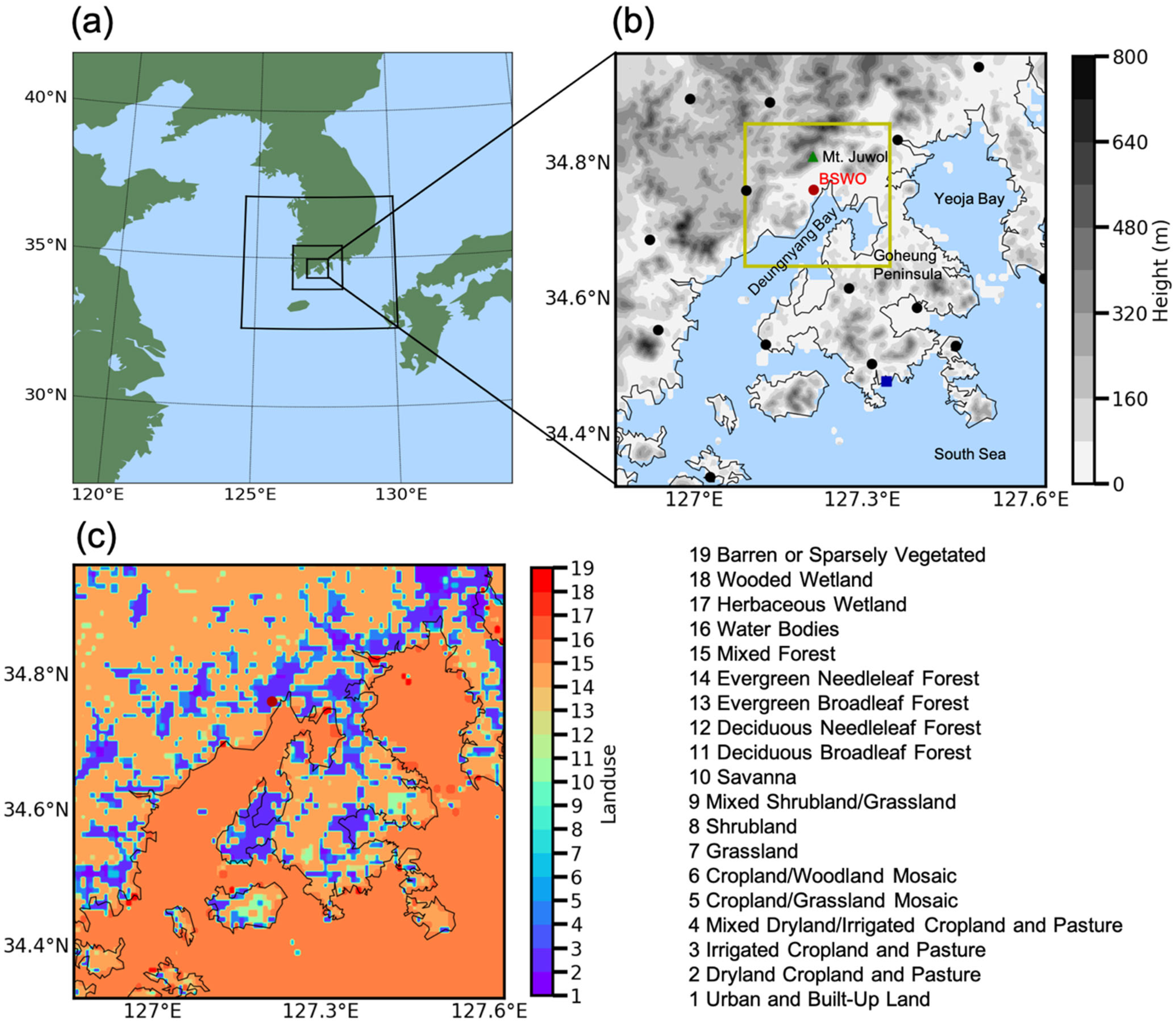
2.1. Site Description and Observations

The BSWO (34°46′ N, 127°13′ E) is located in Boseong in the southern coastal area of the Korean Peninsula (Figure 1). The topography of the BSWO is presented in Figure 1b. The site faces Deungnyang Bay to the southeast; the distance to the bay is ~1.5 km. The bay includes tidal flats that are ~1.2 km wide [16]. The Goheung Peninsula and the South Sea are located to the south of the bay; therefore, this site is influenced by both bay and sea breezes during the daytime. The region within 1.5 km of the BSWO consists of a rice paddy field (Figure 1c). To the north is the 562-meter-high Juwol Mountain. To the west is a narrow valley ~500 m wide that is surrounded by 250-meter-high ridges and connected to the basin area via a narrow gap. The basin area is also connected to other valleys inland. The altitude of the valley floor increases toward the west.

At the BSWO, the air temperature (5628 PRT, Fluke, Everett, WA, USA) and wind speed and direction (2D-UA, Thies, Coesfeld, Germany) were measured at 1-minute intervals at 11 levels (i.e., 10 m, 20 m, 40 m, 60 m, 80 m, 100 m, 140 m, 180 m, 220 m, 260 m, and 300 m) [17]. After quality control, flagless data were used in the analysis. Due to the poor consistency of the 260 m data with data from other levels, we excluded them from the analysis.

In 2018, intensive observation using a radiosonde was conducted at the BSWO every 3 h on 16 consecutive days (2–17 July 2018). We used wind speed, wind direction, and virtual potential temperature from obtained radiosonde data to evaluate the model’s performance in simulating the vertical structure of flow in the boundary layer. Hourly surface wind speed and direction, along with air temperature, from 15 AWS/ASOS stations in domain 4 (D04) were used to evaluate the model. The observed sea surface temperature (SST) at the Goheung-Balpo station (34°29′ N, 127°20′ E) (Figure 1b) was used for comparison with the model-prescribed SST.

2.2. Model Description

We used the WRF model (v.4.1.3) [18], which is a non-hydrostatic, compressible model with a mass coordinate system. Four nested domains with two-way interaction were used in the model configurations (

Table 1. Configuration of the WRF simulation.

Domains	D01	D02	D03	D04
Horizontal resolution (m)	9000	3000	1000	333
Horizontal grid	181 × 181	163 × 163	163 × 163	210 × 210
Microphysics	WRF double-moment 6-class scheme
Surface layer	Revised MM5 Monin–Obukhov scheme
Land surface	Unified Noah land surface model
Longwave radiation	Rapid radiative transfer model scheme
Shortwave radiation	Dudhia scheme
Boundary layer	Shin–Hong scale-aware PBL scheme
Cumulus	Multiscale Kain–Fritsch scheme	-	-	-

). Each domain has 68 vertical layers extending from the ground to 50 hPa. The lowest 20 model sigma levels are at 1.0, 0.997, 0.994, 0.991, 0.988, 0.985, 0.975, 0.97, 0.96, 0.95, 0.94, 0.93, 0.92, 0.91, 0.895, 0.88, 0.865, 0.85, 0.825, and 0.8. The lowest model level is at 13 m above ground level (AGL).

The model was run using 0.25° × 0.25° data from the ERA5 reanalysis data [19] for the initial and lateral boundary conditions. We used topographic data from the high-resolution Shuttle Radar Topography Mission (SRTM)’s 90 × 90 m dataset [20]. The simulation period was 33 h from 15:00 LST on 14 July 2018 to 24:00 LST on 15 July 2018. The first 9 h were used as spin-up periods. Because the simulation period was short, SST update was not considered. The model-prescribed SST was compared with observed SST at Goheung-Balpo. The model-prescribed and the observed daily mean SST were 24.2 °C and 24.9 °C, respectively. Sea-breeze forcing may have been slightly overestimated in the simulation.

For the physics option, we used WRF double-moment 6-class microphysics [21], Dudhia shortwave radiation [22], and rapid radiative transfer model longwave radiation [23]. We used Kain–Fritsch cumulus parameterization [24] only in D01. The Noah land surface model [25] and revised MM5 surface-layer scheme [26] were used for the land surface and surface-layer process, respectively. A 333 m resolution corresponds to the gray zone for the subgrid-scale (SGS) turbulence model [27]. To consider scale-dependent SGS transport in the gray zone, we used the Shin–Hong scale-aware planetary boundary layer (PBL) scheme [28]; in this scheme, nonlocal transport and local transport are treated separately: Nonlocal transport is calculated by multiplying a grid-size dependency function by the total nonlocal transport profile, which is obtained via linear fitting to the large-eddy simulation results. Local transport is formulated by multiplying a grid-size dependency by the total local transport profile, which is calculated using an eddy-diffusivity formula.

2.3. Evaluation

Model performance to simulate temperature and wind speed was evaluated using mean bias error (MBE), root-mean-square error (RMSE), and the index of agreement (IOA) [29]. These statistical indices are computed as follows:

$$\mathrm{MBE}=\frac{{\sum }_{i=1}^N\left(P_i-O_i\right)}{N},$$

(1)

$$\mathrm{RMSE}=\sqrt{\frac{{\sum }_{i=1}^N{\left(O_i-P_i\right)}^2}{N}},$$

(2)

$$\mathrm{IOA}=1.0-\frac{{\sum }_{i=1}^N{\left(O_i-P_i\right)}^2}{{\sum }_{i=1}^N{\left(\left|P_i-\overline{O}\right|+\left|O_i-\overline{O}\right|\right)}^2},$$

(3)

where O_i and P_i are the observed and modeled values of the variables, respectively, and the overbar indicates the mean of the variable. N represents the number of data. IOA varies from 0.0 to 1.0, with higher values indicating better agreement between the modeled and observed results.

Verification of the wind vector is accomplished by computing RMSE_u,v and IOA_u,v between the simulated and observed values:

$${\mathrm{RMSE}}_{u,v}=\sqrt{\frac{{\sum }_{i=1}^N{\left(O_{u,i}-P_{u,i}\right)}^2+{\left(O_{v,i}-P_{v,i}\right)}^2}{N}},$$

(4)

$${\mathrm{IOA}}_{u,v}=1.0-\frac{{\sum }_{i=1}^N{\left(O_{u,i}-P_{u,i}\right)}^2+{\left(O_{v,i}-P_{v,i}\right)}^2}{{\sum }_{i=1}^N{\left(\left|P_{u,i}-\overline{O_u}\right|+\left|O_{u,i}-\overline{O_u}\right|\right)}^2+{\left(\left|P_{v,i}-\overline{O_v}\right|+\left|O_{v,i}-\overline{O_v}\right|\right)}^2},$$

(5)

where O_u,i and P_u,i are the observed and simulated u components of the wind speed, respectively. Similarly, O_v,i and P_v,i are the correspondents for the v components.

2.4. Sea-Breeze Characteristics

We define sea-breeze characteristics as described by Lim and Lee [14]. At our study site, bay and sea breezes coexist, but it is difficult to differentiate them in observations. Therefore, we do not differentiate them, and refer to both as sea breeze.

• Onset (LST): The onset is the time when the sea-breeze front (SBF) passes. The time of SBF passage is defined as the time when the wind direction at 10 m AGL changes from offshore or weak wind (wind speed ≤ 1.5 m s⁻¹) to onshore flow (60°–240°) after sunrise, and when the change in wind direction is greater than 30° over the course of an hour;
• Cessation (LST): The cessation is the time when the sea breeze ends. The cessation happens when the wind speed at 10 m AGL is ≤1.5 m s⁻¹, or when the wind is an offshore flow between 15:00 and 24:00 LST. Before offshore flow, the previous wind must be blown onshore;
• Depth of sea breeze: The depth of onshore flow with a speed ≥1.5 m s⁻¹;
• Intensity of sea breeze: The wind speed of the sea breeze.
• We calculate the sea-breeze characteristics by using 10-minute moving-average data for both simulation and observation.

2.5. Design of Sensitivity Experiment

To analyze the effects of horizontal and vertical resolution on the simulated flow structure, we performed three additional sensitivity experiments using different horizontal and vertical resolutions (

Table 2. Design of sensitivity simulations.

Experiment	Horizontal Resolution (m)	Vertical Resolution (Levels)
S03	1000	60
S03V	1000	68
S04	333	60
S04V (Default)	333	68

). In the names of the experiments, “03” and “04” represent the experiments where the innermost domain has a horizontal resolution of 1000 m and 333 m, respectively, and “V” indicates the experiments with increased vertical resolution in the ABL. The experiments without “V” in the name resolve 11 vertical levels below 2 km AGL, while those with “V” resolve 19 vertical levels below 2 km AGL.

3. Observations and Model Evaluation

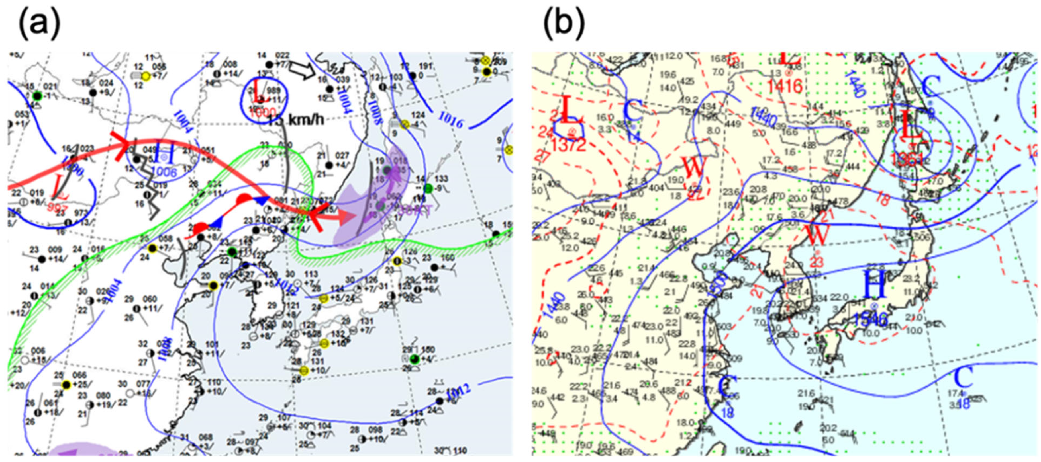
3.1. General Meteorological Conditions for 15 July 2018

Out of the 16 days of the IOP, we selected 15 July 2018 as a case study day. On that day, the synoptic flow was very weak, and the sky was clear, providing favorable conditions for the occurrence of local winds such as sea breezes [30] and along-valley winds. The surface weather map at 09:00 LST on the study day (Figure 2a) shows the North Pacific High fully expanded toward the Korean Peninsula, and weak pressure gradients over Korea. The stationary “Changma” front moved to northeastern China. South Korea was under a clear sky with a warm and humid air mass. This is a typical synoptic pattern after “Changma” in summer in South Korea. The 850 hPa weather chart shows the North Pacific High with the highest pressure zones over Japan and weak clockwise winds over South Korea (Figure 2b). The radiosonde observation showed that the wind direction was 207° and wind speed was 0.2 m s⁻¹ on the 850 hPa level at 09:00 LST. Sunrise occurred at 05:28 LST, and sunset at 19:45 LST.

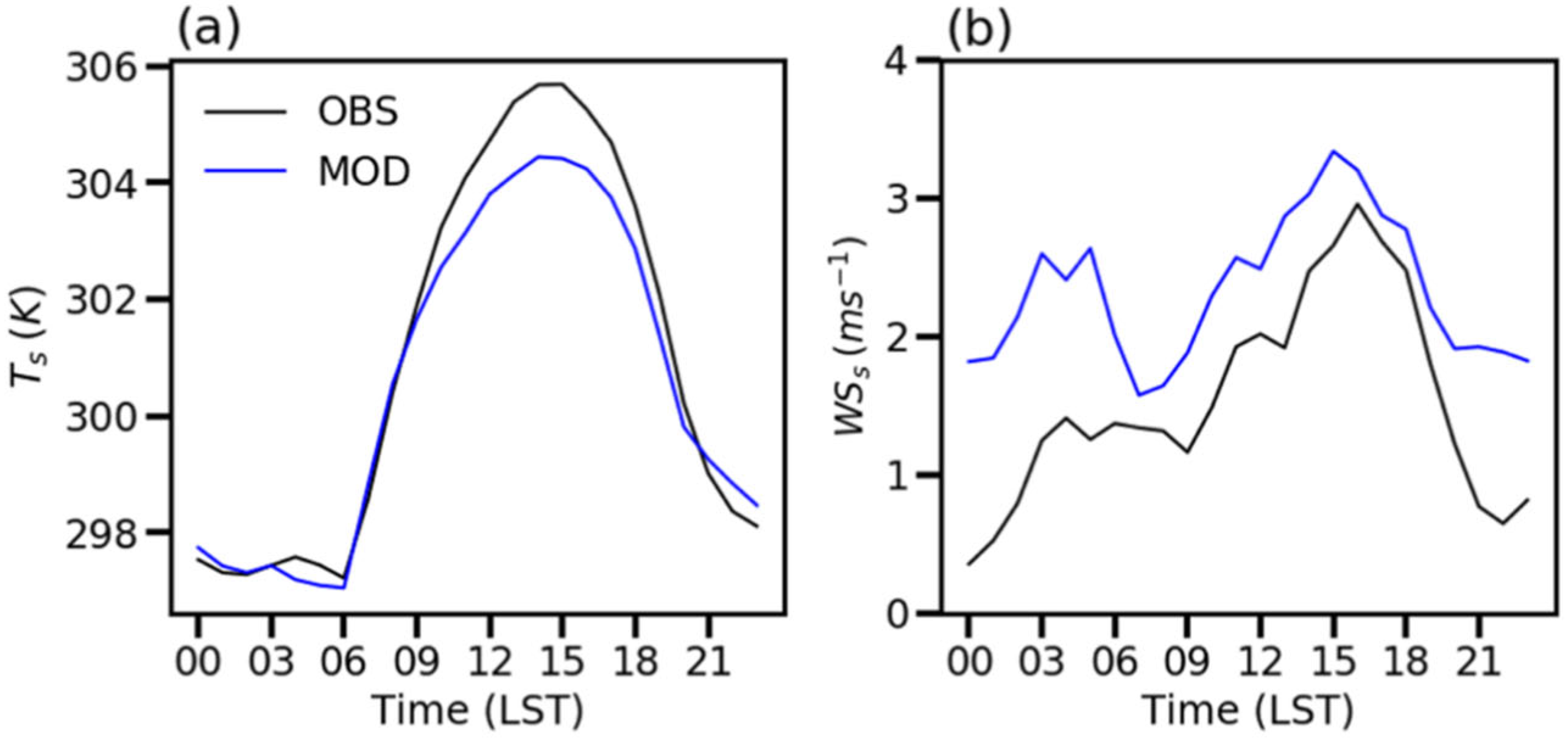
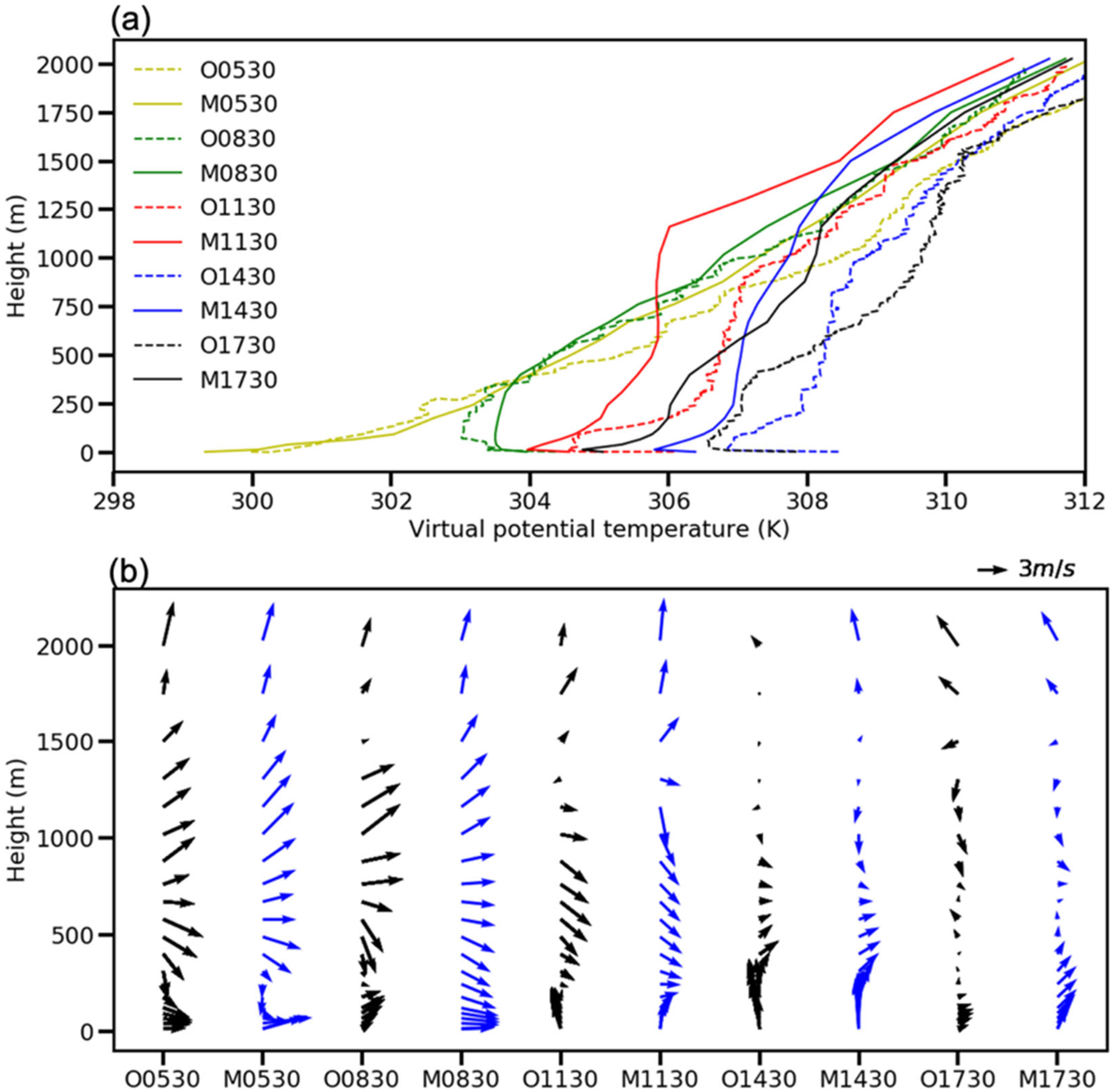
3.2. Model Evaluation

Figure 3 shows the mean diurnal variation of near-surface temperature (T_s) and wind speed (WS_s) for the default simulation (S04V) and observations at 15 AWS/ASOS stations within D04 for the study day. The evaluation statistics for the variables (

Table 3. Model evaluation statistics for near-surface variables against the observations from 15 AWS/ASOS stations in D04 on 15 July 2018. MBE, RMSE, and IOA indicate the mean bias error, root-mean-square error, and index of agreement, respectively. N represents the number of data.

N	2-m Air Temperature			10-m Wind Speed			10-m Wind Vector
	MBE (K)	RMSE (K)	IOA	MBE (m s−1)	RMSE (m s−1)	IOA	RMSEu,v (m s−1)	IOAu,v
360	−0.43	1.28	0.95	0.91	1.56	0.62	2.22	0.71

) indicate that the model underestimates the daytime T_s, but closely reproduces diurnal amplitude for T_s. However, overall overestimation is shown for the wind speed, particularly during nighttime (Figure 3b). Figure 4a shows the horizontal distribution of the simulated T_s and wind vectors with observed wind vectors at 03:00 LST. The simulation shows strong northwesterly land-breezes near the coast, whereas the observation shows weak land breezes at a few coastal sites, and calm winds at most sites. Overestimation of land-breeze intensity has been reported in previous modeling studies [31]. One possible cause for the nighttime wind speed overprediction is that the resolution used does not resolve small-scale valleys and hills. At night, the valley atmosphere is decoupled from the air aloft because the stable structure within the valley suppresses the vertical exchange of air between the valley and above the valley. Surrounding hills also shelter the valley’s atmosphere from the wind aloft [32], weakening the observed wind speed within valleys. Figure 4b shows the horizontal distribution of the simulated T_s and wind vectors with observed wind vectors at 15:00 LST. In the South Sea, southwesterly flows blow parallel to the large-scale coastline, while in the bay, southwesterly and southerly flows blow in due to differential heating between the bay and the South Sea. The direction of the sea breeze at each station depends on the orientation of the local coast. The observed wind vectors are well reproduced in the model at 15:00 LST. The evaluation statistics show that the model simulates T_s and wind reasonably well (Table 3).

We evaluated the vertical structure of the ABL at the BSWO against radiosonde data. Figure 5 displays the vertical profiles of the observed virtual potential temperature and wind vectors at 3-hour intervals from 05:30 LST to 17:30 LST below 2 km AGL, and the corresponding S04V outputs.

Table 4. Model evaluation statistics for the 3-hourly vertical profiles of virtual potential temperature and winds below 2 km AGL against the observations from the radiosonde at the BSWO from 05:30 to 17:30 LST on 15 July 2018. MBE, RMSE, and IOA indicate the mean bias error, root-mean-square error, and index of agreement, respectively. N represents the number of data.

Time (LST)	N	Virtual Potential Temperature			Wind Speed			Wind Vector
		MBE (K)	RMSE (K)	IOA	MBE (m s−1)	RMSE (m s−1)	IOA	RMSEu,v (m s−1)	IOAu,v
0530	20	−0.34	0.65	0.99	0.39	1.16	0.51	1.51	0.86
0830	20	−0.04	0.36	0.99	1.03	1.68	0.42	2.29	0.62
1130	20	−1.08	1.22	0.85	0.54	0.92	0.74	1.55	0.91
1430	20	−1.13	1.18	0.74	0.41	0.97	0.89	1.3	0.92
1730	20	−1.29	1.36	0.81	0.82	1.55	0.20	1.95	0.73

summarizes the evaluation statistics of the vertical profiles of the variables at 3-hour intervals from 05:30 to 17:30 LST. For evaluation, we sampled radiosonde observations at the 20 altitudes nearest to the vertical grid levels of S04V below 2 km AGL.

At 05:30 LST, observations show that strong surface inversion is formed with near-surface westerly flow, which is well captured in S04V (Figure 5a), showing an IOA of 0.99 for virtual potential temperature. Above 300 m AGL, counterclockwise rotation of wind with height appears in both observation and S04V (Figure 5b). Large differences in wind vectors between the model results and observations are shown at 08:30 LST. The model does not reproduce wind decoupling at 250 m AGL, which clearly appears in observation; this discrepancy could be explained by the difference in thermal structure. Observations show shallow superadiabatic layers near the surface with strong inversion above, leading to decoupling between near-surface air and upper-level flow. In contrast, the model simulates the well-mixed thermal structure below 500 m AGL, allowing well-coupled conditions with upper-level westerly flows.

A cold bias is shown in the entire layer at 11:30 LST, and continues in the afternoon. The simulated surface sensible heat flux is overestimated in the morning (figure not shown here), suggesting that surface forcing is not the main cause of the cold bias. Cooling above 1250 m AGL between 08:30 and 11:30 LST, presumably due to cold advection, is noted in the simulation. Cooling in the above PBL also contributed to cold bias within the PBL through the entrainment process. At 14:30 LST, the vertical extent of the observed sea breeze is about 508 m and return flow is very weak, which is well captured in the simulation (Table 4). The vertical extent of sea breeze at this site is comparable to the sea breeze depth of 500–1000 m reported in other regions [33,34]. During 14:30–17:30 LST, the observed potential temperature increases between 500 and 1500 m AGL and decreases below 500 m AGL, indicating that cooling occurs below 500 m AGL. Such features are well captured in the simulation. S04V well reproduces the flow pattern for upper 500 m AGL but simulates southwesterly sea breezes below 500 m AGL unlike observed westerlies.

4. Analysis of Numerical Simulation and Discussion

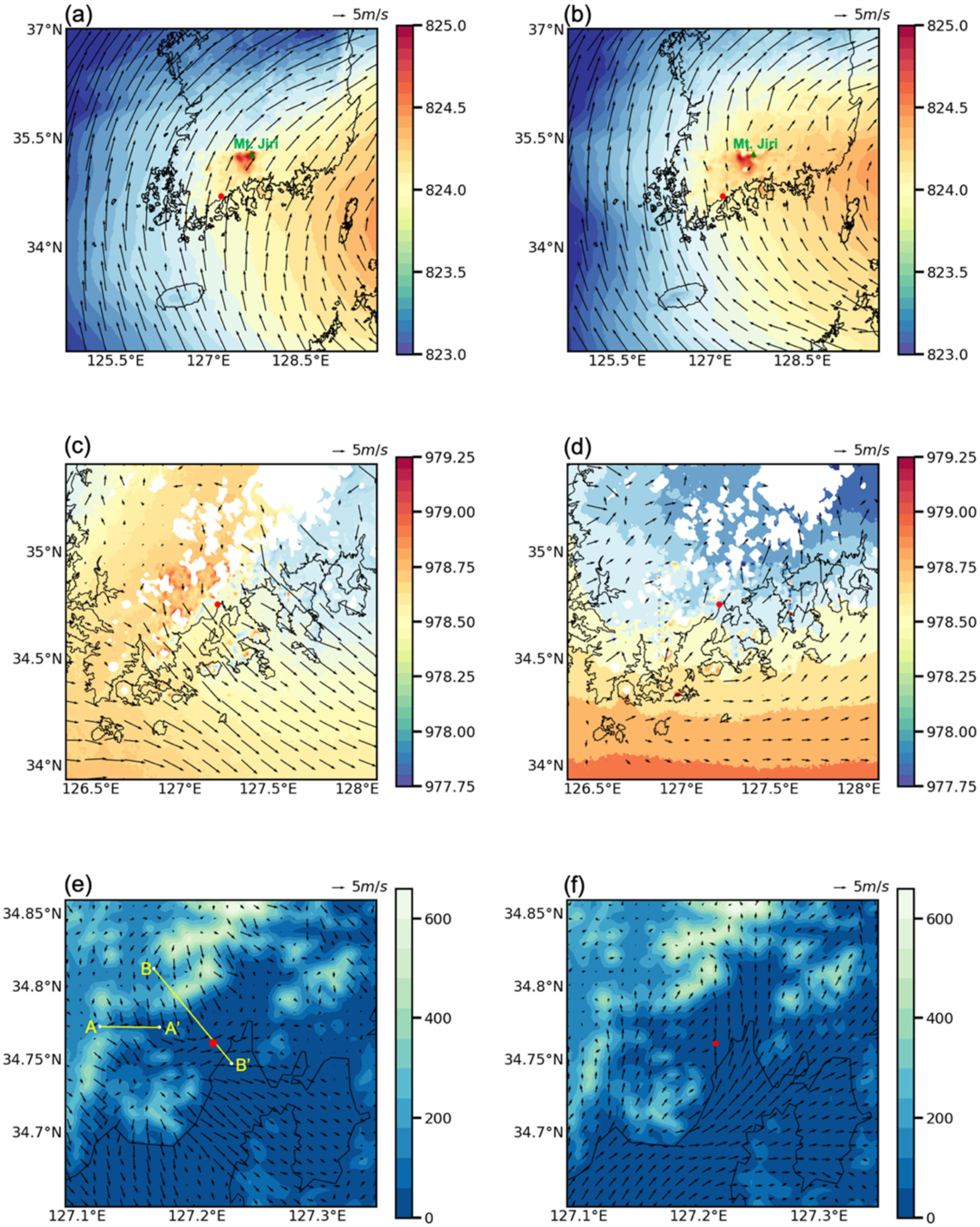
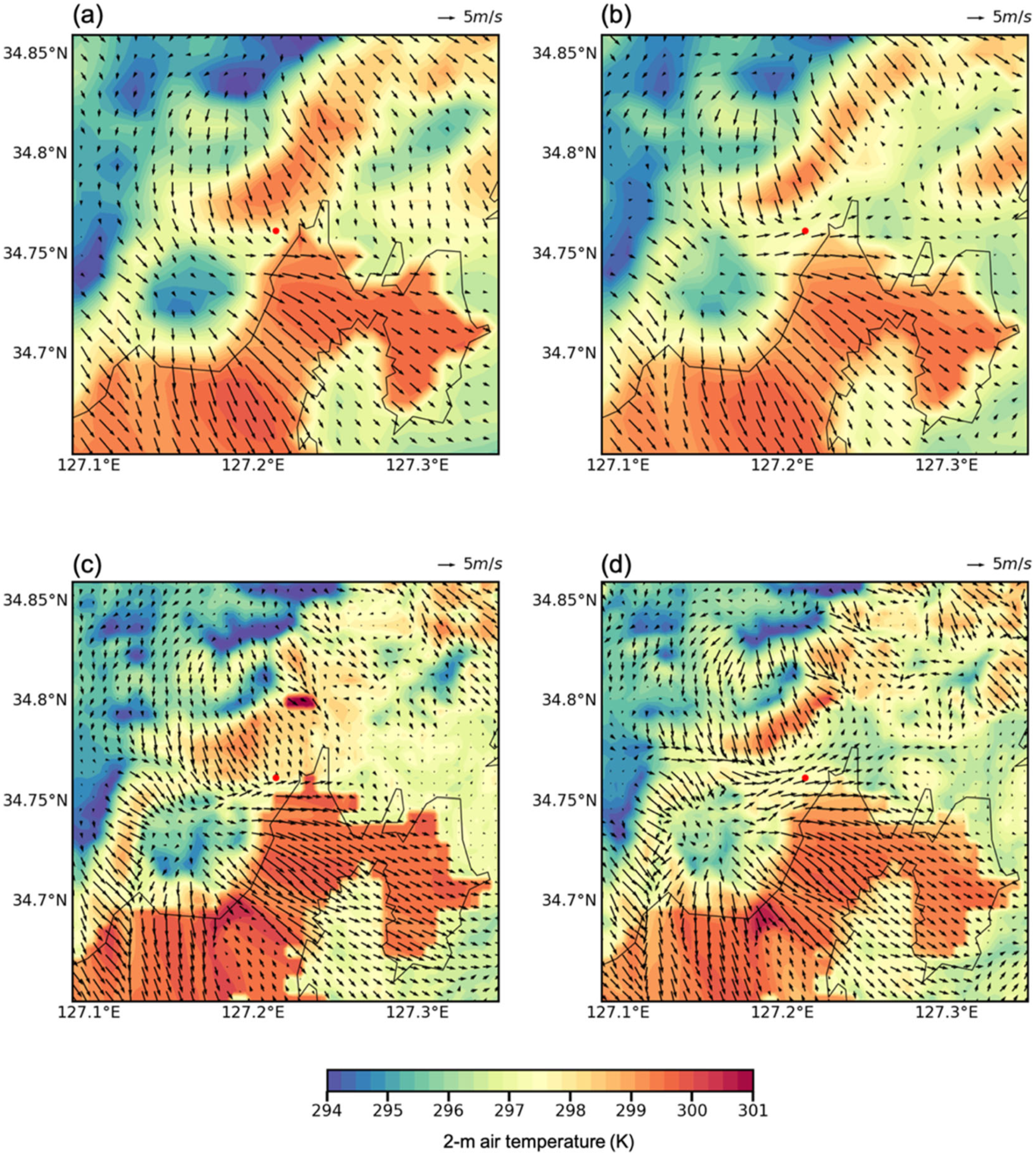
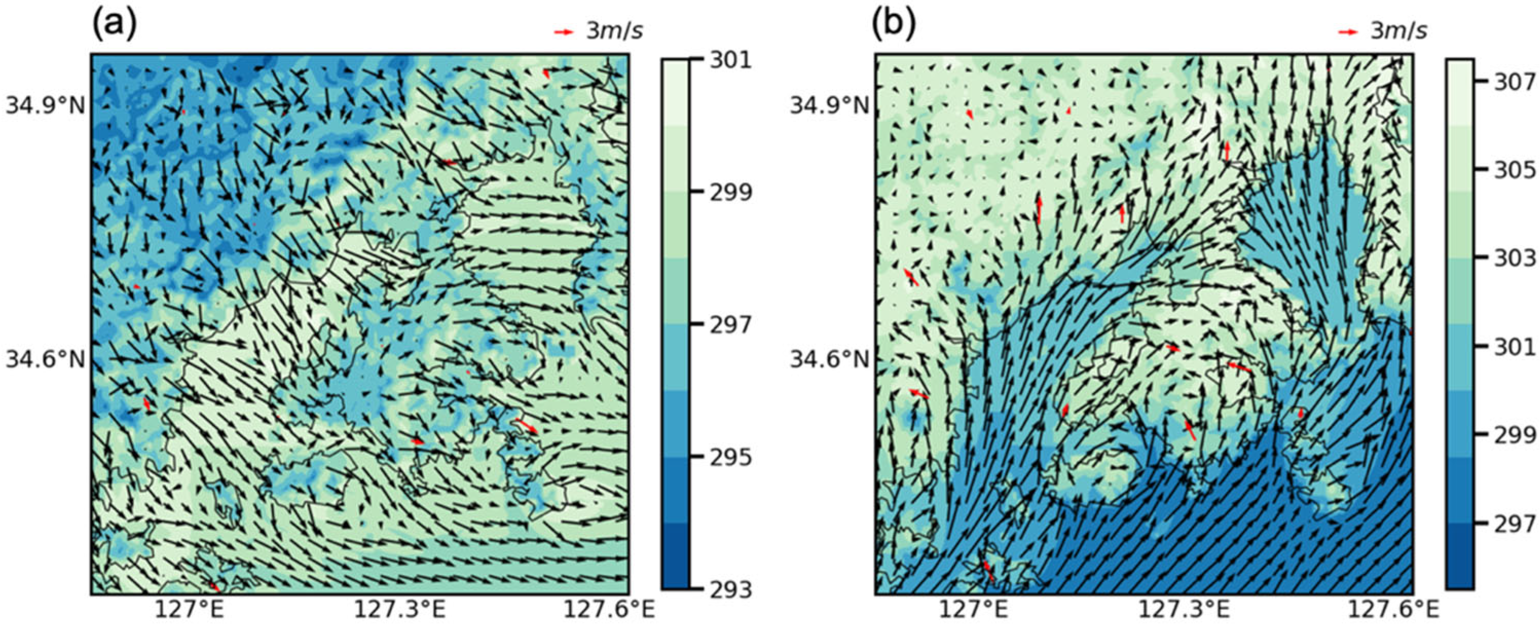
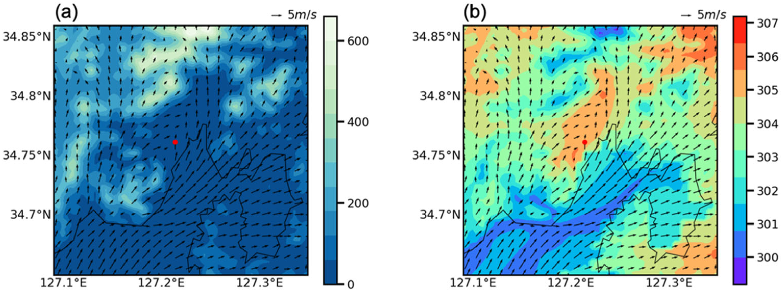
4.1. Regional-Scale Description of the Flows

The complex layering of the atmosphere at the BSWO is confirmed by observational data. To understand and interpret these structures, we analyzed modeling results at 05:30 and 14:30 LST, when the model’s performance for the vertical sounding of wind vectors was good (Table 4). Figure 6a,b show the horizontal wind field superposed over the pressure field at 1800 m AGL at 05:30 and 14:30 LST, respectively, in D02. At 05:30 LST, the pressure pattern is dominated by the North Pacific High, and clockwise rotation of wind surrounding the North Pacific High is shown, leading to southwesterly flow above the BSWO. On the other hand, at 14:30 LST, heating over the land leads to a wide high-pressure zone over land, and divergent flow is noted surrounding Mt. Jiri. The resulting mesoscale pressure gradient partially counteracts the synoptic pressure gradient, leading to a weak pressure gradient and, hence, weak wind at 1800 m AGL above the BSWO. Figure 6c,d show the horizontal wind field with the pressure field at 300 m AGL at 05:30 and 14:30 LST, respectively, in D03. At 05:30 LST, the cold and dense air is found over the interior of the land, whereas temperatures on the sea side are moderated by the sea (figure not shown), leading to high pressure inland of elevated areas and low pressure on their coastal sides. The wind blows from high pressure to low pressure near the coast, leading to northwesterly flow at 300 m AGL above the BSWO. Therefore, baroclinicity due to topography explains the counterclockwise rotation of wind vectors with height above 300 m AGL in Figure 5b. At 14:30 LST, a thermal low forms surrounding elevated areas over land, and a thermal high exists in the South Sea, leading to southwesterly flow at the BSWO. Figure 6e,f show the horizontal wind field at 10 m AGL with topography at 05:30 and 14:30 LST, respectively, in the analysis domain. The near-surface westerly flow at the BSWO is connected to along-valley flows to the west of the BSWO at 05:30 LST. At 14:30 LST, a southerly sea breeze penetrates inland at the BSWO, and underlying terrain shifts its direction from southerly to southwesterly to the west of the BSWO.

To examine the mechanisms of flow structure below 300 m AGL at 05:30 LST, we examined the vertical cross-section of wind and virtual potential temperature along the lines AA′ and BB′ in Figure 6e. The air within the valley is colder than the air at the same altitude over the plain, and cold air flows along the valley into the plain, leading to down-valley wind [32] (Figure 7a). The down-valley wind brings cold air from the valley to the plain, contributing to cooling over the plain. Figure 7b shows the vertical cross-section of wind and virtual potential temperature along the line BB′. The wind vectors parallel to the line BB′ are displayed in Figure 7b. Near-surface flow in the windward direction is blocked by the mountain, and the wind is very weak, leading to subcritical flow windward of the mountain. As a subcritical flow ascends the upslope side of a mountain, the Froude number (Fr) tends to increase [35]. If Fr = 1 at the crest, the flow becomes supercritical and continues to accelerate as it descends on the lee slope, until a hydraulic jump occurs. Figure 7b shows strong downslope flow on the lee slope and sudden cessation of the wind near the foot of the mountain. We examined the variation in wind speed at 38 m AGL and the layer thickness between the surface and 303 K along BB′. The wind speed increase was accompanied by a decrease in layer thickness, and in the lee of the mountain, the sudden increase in layer thickness corresponds to the sudden decrease in wind speed. This shows a typical pattern of supercritical flow on lee slopes, with adjustment to subcritical flow at a hydraulic jump near the foot of the mountain [35], suggesting that the calm wind between 200 and 300 m AGL observed at 05:30 LST is explained by hydraulic jump. The increase in wind speed at the BSWO is due to westerly down-valley wind (Figure 6e). Based on the results, we suggest that the observed LLWM in the early morning is produced by near-surface down-valley wind and weak wind due to a hydraulic jump above the down-valley wind.

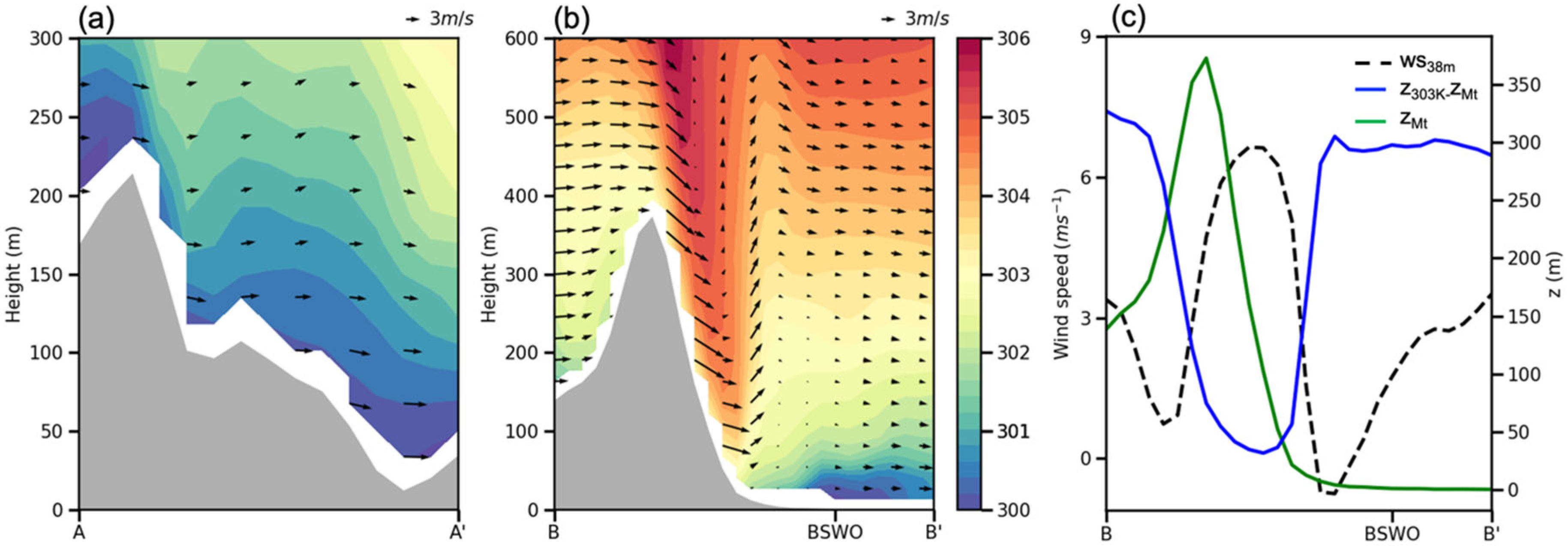
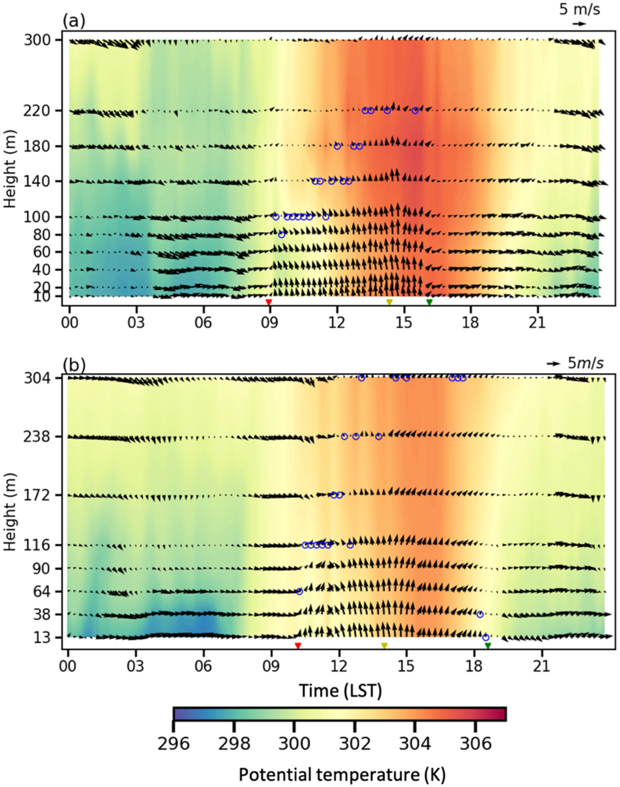
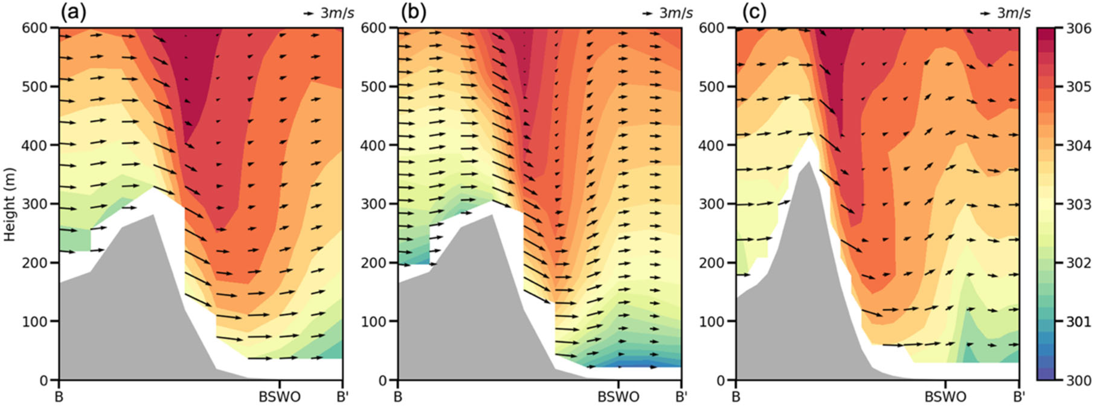
4.2. Down-Valley Wind and Sea Breeze at BSWO

Figure 8 shows the time–height cross-section of the wind and potential temperature at the BSWO on the study day for the 300 m tower observations and S04V. Before 03:00 LST, S04V simulates the observed calm wind below 100 m AGL well, which precedes the westerly down-valley wind. The calm wind results in strong stratification near the surface, leading to a decoupling of the down-valley flow from the upper-level flow [36]. Before the calm wind appears above the down-valley flow, the wind at 300 m AGL changes from westerly to northwesterly, leading to flow over the mountains. At 07:00 LST, the depth and mean intensity of the observed down-valley wind (240°–300°) are 180 m and 3.7 m s⁻¹, respectively. S04V simulated down-valley wind but underestimated its depth (116 m) and mean intensity (2.2 m s⁻¹), resulting in less cooling below 300 m AGL than was observed.

The onset of sea breeze in the S04V simulation occurs ~1 h later than observed. In the model, the strong westerly flow delays the onset of the sea breeze. Such blocking of onset by opposing flow has been reported in previous studies [10]. The sea-breeze depths are well captured in the simulation (Figure 8). The observed maximum sea-breeze intensity is 6.3 m s⁻¹, which occurs at 20 m AGL at 14:22 LST; the corresponding simulated value is 5.7 m s⁻¹ at 13 m AGL at 14:02 LST. At 16:09 LST, the observed wind shifts from southerly to westerly, leading to the cessation of the sea breeze. S04V also captures a wind shift from southerly to southwesterly around 15:30 LST, but the changes in wind direction are not as large as those leading to cessation, which occurs around 2 h later (18:36 LST). The later cessation of sea breeze causes an additional cooling in the late afternoon, leading to lower temperature in the simulation than in the observations.

To understand the sudden wind shift observed at 16:00 LST, we examined the horizontal distribution of simulated 10-m wind with topography and 2-m air temperature in the analysis domain at 16:00 LST (Figure 9). Southerly and southwesterly sea breezes are shown over land. Topography plays a role in such flow diversion over land. Relatively warm temperatures in the flat plain also contribute to the wind turning from southwesterly to westerly flow. At the BSWO, sea breeze blows as a southerly flow, converging with a southwesterly sea breeze in relatively warm regions. The model simulates a shift of southerly to westerly flow, but with a slight location error. The simulated southerly sea breeze is stronger than observed. Possible causes for larger sea-breeze forcing in the simulation are lower SST and neglect of changing tide state. On the study day, low tide occurred at 17:00 LST. Lee showed that sea-breeze intensity at this site decreases early when low tide occurs in the afternoon [16]. Low tide in the afternoon may also contribute to less cooling by sea breeze being observed after 15:00 LST than in the simulation, because the air blows from exposed mud and shallow water.

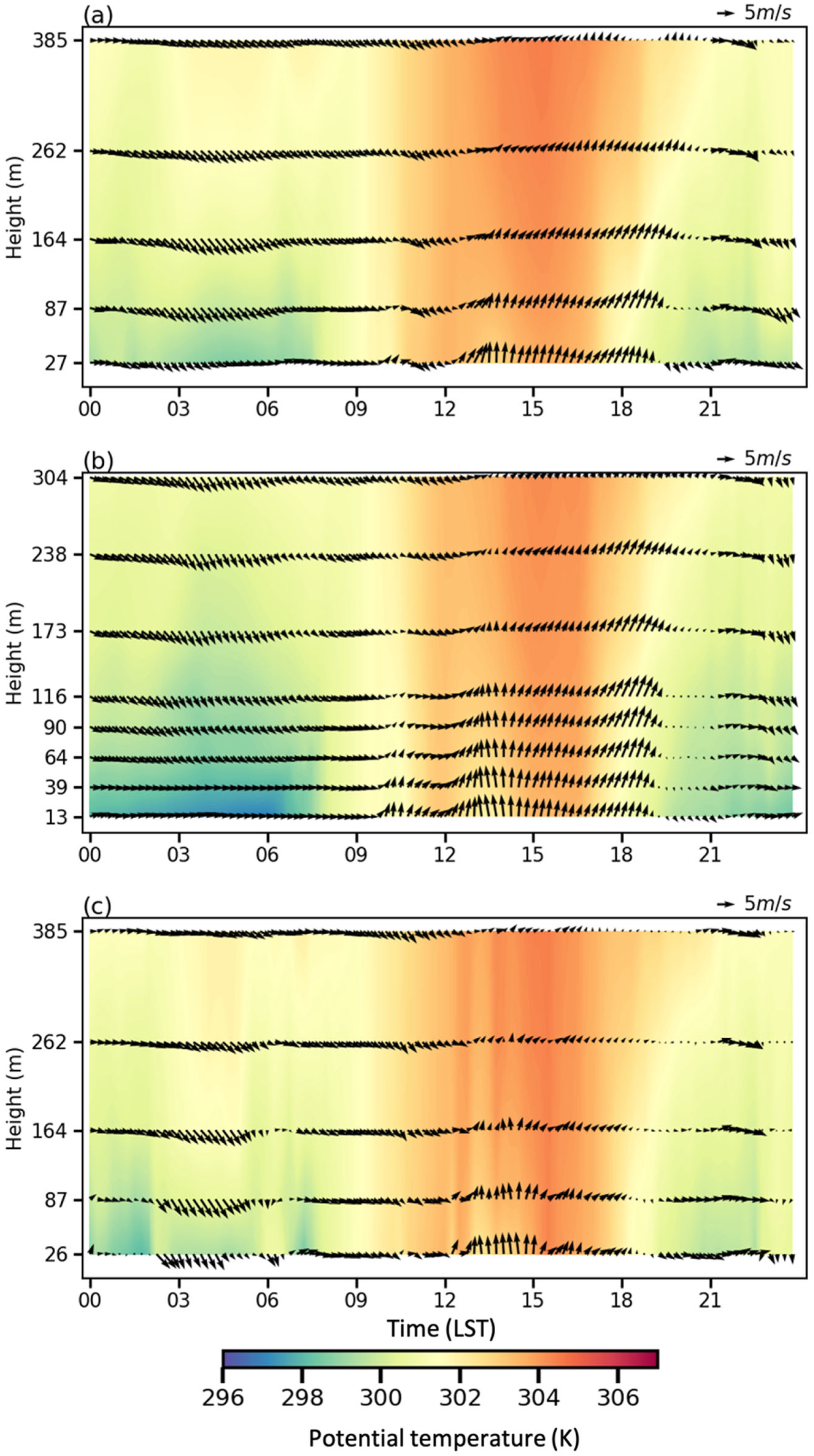
4.3. Sensitivity of Simulated Flow Structure to Model Resolution

In this section, we examine the sensitivity of the simulated flow structure to the model resolution. Figure 10 shows the time–height cross-section of potential temperature and wind vectors at the tower site for sensitivity simulations. None of the sensitivity simulations show calm winds between 200 and 300 m AGL in the early morning. The differences in thermal structure between sensitivity simulations are more evident during nighttime than daytime. Colder temperatures below 200 m AGL in the early morning are shown in the simulations using high vertical resolution (S03V and S04V). The onset of the sea breeze occurs later in simulations with low vertical resolution (S03 and S04) (

Table 5. The simulated characteristics of sea breeze on 15 July 2018.

Variables	S04V	S04	S03V	S03
Onset (LST)	1011	1207	0951	1257
Cessation (LST)	1836	1707	1902	1912

). The model using high vertical resolution better simulates stable stratification under a penetrating sea breeze, allowing a sharp sea-breeze front near the surface, and also reducing the influence of upper-level flow on the sea breeze. However, the dependence of onset on the horizontal resolution is not consistent in this study case; more analysis is required on this matter. On the other hand, the cessation of the sea breeze occurs later in simulations with low horizontal resolution; this is because shifts in wind direction leading to sea-breeze cessation at this site are better simulated at a high horizontal resolution, which better resolves the topography.

To examine the causes of the different flows and thermal structures in the early morning related to model resolution, we examined the simulated horizontal distribution of 10-m wind vectors and 2-m air temperatures at 05:30 LST (Figure 11). The simulated temperature distributions show low temperatures over elevated areas and high temperatures over sea and downslope regions. The temperature differences in the flat plain near the study site between simulations should be noted. Higher temperatures are shown in S03 and S04 than in their counterparts S03V and S04V; such temperature differences could be explained in terms of wind difference. The flat plain near the study site is influenced by northwesterly flow in S03 and S04, but by westerly flow in S03V and S04V. Because the northwesterly flow is downslope flow over a mountain, air temperature increases due to adiabatic heating during downward motion. In contrast, westerly flow originates from the valley with cold air. Figure 12 shows the vertical cross-section of virtual potential temperature and wind along the line BB′ from sensitivity simulations. In S03, with smooth topography and low vertical resolution, a mountain wave is simulated when stable air flows over the mountain, and northwesterly flow extends to the BSWO. The use of high vertical resolution in S03V allows the model to simulate stable stratification near the surface, which prevents northwesterly flow from reaching the BSWO near the surface. On the other hand, the use of high horizontal resolution in S04 allows steep slopes of the mountain, producing a thinner and stronger downslope flow in the lee of the mountain, but stable stratification near the surface and the sudden increase in layer thickness in the lee of mountain are not well simulated. These results indicate that both high vertical resolution and high horizontal resolution are required in order to simulate a hydraulic jump in the lee of a mountain.

5. Summary

We evaluated the performance of the high-resolution WRF model in simulating the thermal and flow structure of the ABL for a sea-breeze event on 15 July 2018 against observations taken from AWS/ASOS, a 300 m tower and radiosonde. The model showed good performance in simulating near-surface air temperatures and wind vectors in D04, as well as the vertical structure of potential temperatures and wind vectors at the BSWO in the ABL. The simulated sea-breeze features such as onset and cessation at the BSWO were compared with observations obtained from a 300 m tower. Although the model simulated the onset of sea breeze ~1 h later than observed, the vertical extent of the sea breeze was well reproduced. At 16:00 LST, observation showed a rapid wind shift from southerly to westerly due to the local topography, leading to the cessation of the sea breeze. Although the model simulated such shifts in wind direction with a small location error, it simulated cessation 2 h later at the study site.

To interpret the measurements, we analyzed the modeled results at 05:30 and 14:30 LST, when the model’s performance was good for wind. The counterclockwise wind rotation with height above 300 m AGL at 05:30 LST can be explained by baroclinicity due to topography. The observed LLWM at 05:30 LST was well simulated in the model. The modeled results show that a hydraulic jump produces weak wind conditions below 300 m AGL, and westerly down-valley flow develops near the surface, leading to an LLWM. At 14:30 LST, heating over land produces a thermal high over land at 1800 m AGL, which counteracts the synoptic pressure gradient and, thus, leads to weak wind conditions at this level.

We performed three sensitivity simulations to examine the dependence of boundary layer flow and thermal structure on model resolution. A vertical high-resolution model better simulates stable stratification near the surface, and shows better performance in simulating the onset of sea breeze. A horizontal high-resolution model better simulates the local change in wind direction due to topography. To properly simulate the hydraulic jump in the lee of a mountain, both high horizontal and high vertical resolutions are required.

The results of this study are helpful in understanding the flow and thermal structure of the ABL in complex coastal sites on a clear day under weak synoptic wind conditions. High-resolution model results suggest the presence of mesoscale phenomena such as strong downslope winds and hydraulic jumps in the boundary layer in complex terrain. Good forecasting of these phenomena is important for the safe operation of urban air mobility in the boundary layer in the future. Our results are based on model results and vertical profile measurements at only one site. To verify the presence of the phenomena, detailed observations following the slope of a mountain are required in the future. In addition, more modeling studies with long-term data are needed in order to draw general conclusions about the flow structure in complex areas.

References

1. Glickman, T.S. Glossary of Meteorology, 2nd ed.; American Meteorological Society: Boston, MA, USA, 2000; p. 855. [Google Scholar]
2. Baklanov, A.A.; Grisogono, B.; Bornstein, R.; Mahrt, L.; Zilitinkevich, S.S.; Taylor, P.; Larsen, S.E.; Rotach, M.W.; Fernando, H.J.S. The Nature, Theory, and Modeling of Atmospheric Planetary Boundary Layers. Bull. Am. Meteorol. Soc. 2011, 92, 123–128. [Google Scholar] [CrossRef] [Green Version]
3. LeMone, M.A.; Angevine, W.M.; Bretherton, C.S.; Chen, F.; Dudhia, J.; Fedorovich, E.; Katsaros, K.B.; Lenschow, D.H.; Mahrt, L.; Patton, E.G.; et al. 100 Years of Progress in Boundary Layer Meteorology. Meteorol. Monogr. 2019, 59, 9.1–9.85. [Google Scholar] [CrossRef]
4. Steiner, M. Urban Air Mobility: Opportunities for the Weather Community. Bull. Am. Meteorol. Soc. 2019, 100, 2131–2133. [Google Scholar] [CrossRef]
5. Haupt, S.E.; Rauber, R.M.; Carmichael, B.; Knievel, J.C.; Cogan, J.L. 100 Years of Progress in Applied Meteorology. Part I: Basic Applications. Meteorol. Monogr. 2018, 59, 22.1–22.33. [Google Scholar] [CrossRef]
6. Stith, J.L.; Baumgardner, D.; Haggerty, J.; Hardesty, R.M.; Lee, W.-C.; Lenschow, D.; Pilewskie, P.; Smith, P.L.; Steiner, M.; Vömel, H. 100 Years of Progress in Atmospheric Observing Systems. Meteorol. Monogr. 2018, 59, 2.1–2.55. [Google Scholar] [CrossRef]
7. Michener, W.K.; Blood, E.R.; Bildstein, I.K.L.; Brinson, M.M.; Gardner, L.R. Climate Change, Hurricanes and Tropical Storms, and Rising Sea Level in Coastal Wetlands. Ecol. Appl. 1997, 7, 770–801. [Google Scholar] [CrossRef]
8. Bastin, S.; Drobinski, P. Sea-Breeze-Induced Mass Transport over Complex Terrain in South-Eastern France: A Case-Study. Q. J. R. Meteorol. Soc. 2006, 132, 405–423. [Google Scholar] [CrossRef] [Green Version]
9. Pérez-Landa, G.; Ciais, P.; Sanz, M.J.; Gioli, B.; Miglietta, F.; Palau, J.L.; Gangoiti, G.; Millán, M.M. Mesoscale Circulations over Complex Terrain in the Valencia Coastal Region, Spain—Part 1: Simulation of Diurnal Circulation Regimes. Atmos. Chem. Phys. 2007, 7, 1835–1849. [Google Scholar] [CrossRef] [Green Version]
10. Arrillaga, J.A.; Yagüe, C.; Sastre, M.; Román-Cascón, C. A Characterisation of Sea-Breeze Events in the Eastern Cantabrian Coast (Spain) from Observational Data and WRF Simulations. Atmos. Res. 2016, 181, 265–280. [Google Scholar] [CrossRef]
11. Caicedo, V.; Rappenglueck, B.; Cuchiara, G.; Flynn, J.; Ferrare, R.; Scarino, A.J.; Berkoff, T.; Senff, C.; Langford, A.; Lefer, B. Bay Breeze and Sea Breeze Circulation Impacts on the Planetary Boundary Layer and Air Quality from an Observed and Modeled DISCOVER-AQ Texas Case Study. J. Geophys. Res. Atmos. 2019, 124, 7359–7378. [Google Scholar] [CrossRef]
12. Ryu, Y.-H.; Baik, J.-J. Daytime Local Circulations and Their Interactions in the Seoul Metropolitan Area. J. Appl. Meteorol. Climatol. 2013, 52, 784–801. [Google Scholar] [CrossRef]
13. Hughes, C.P.; Veron, D.E. A Characterization of the Delaware Sea Breeze Using Observations and Modeling. J. Appl. Meteorol. Climatol. 2018, 57, 1405–1421. [Google Scholar] [CrossRef]
14. Lim, H.-J.; Lee, Y.-H. Characteristics of sea breezes at coastal area in Boseong. Atmosphere 2019, 29, 41–51. [Google Scholar] [CrossRef]
15. Lee, Y.-H. Climatology of Nocturnal Low-Level Wind Maxima at a Topographically Complex Coastal Site in Boseong. Meteorol. Atmos. Phys. 2021, 133, 643–653. [Google Scholar] [CrossRef]
16. Lee, Y.-H. Observational Analysis of Tidal Effect on Sea Breeze. Bound.-Layer Meteorol. 2021, 180, 273–288. [Google Scholar] [CrossRef]
17. Korea Meteorological Administration. Application of Boseong Global Standard Observatory (I); NIMR-2014-B-11; Korea Meteorological Administration: Seoul, Korea, 2014; pp. 1–128.
18. Skamarock, W.C.; Klemp, J.B. A Time-Split Nonhydrostatic Atmospheric Model for Weather Research and Forecasting Applications. J. Comput. Phys. 2008, 227, 3465–3485. [Google Scholar] [CrossRef]
19. Hersbach, H.; Bell, B.; Berrisford, P.; Hirahara, S.; Horányi, A.; Muñoz-Sabater, J.; Nicolas, J.; Peubey, C.; Radu, R.; Schepers, D.; et al. The ERA5 Global Reanalysis. Q. J. R. Meteorol. Soc. 2020, 146, 1999–2049. [Google Scholar] [CrossRef]
20. Farr, T.G.; Rosen, P.A.; Caro, E.; Crippen, R.; Duren, R.; Hensley, S.; Kobrick, M.; Paller, M.; Rodriguez, E.; Roth, L.; et al. The Shuttle Radar Topography Mission. Rev. Geophys. 2007, 45. [Google Scholar] [CrossRef] [Green Version]
21. Lim, K.-S.S.; Hong, S.-Y. Development of an Effective Double-Moment Cloud Microphysics Scheme with Prognostic Cloud Condensation Nuclei (CCN) for Weather and Climate Models. Mon. Weather Rev. 2010, 138, 1587–1612. [Google Scholar] [CrossRef] [Green Version]
22. Dudhia, J. Numerical Study of Convection Observed during the Winter Monsoon Experiment Using a Mesoscale Two-Dimensional Model. J. Atmos. Sci. 1989, 46, 3077–3107. [Google Scholar] [CrossRef]
23. Mlawer, E.J.; Taubman, S.J.; Brown, P.D.; Iacono, M.J.; Clough, S.A. Radiative Transfer for Inhomogeneous Atmospheres: RRTM, a Validated Correlated-k Model for the Longwave. J. Geophys. Res. Atmos. 1997, 102, 16663–16682. [Google Scholar] [CrossRef] [Green Version]
24. Kain, J.S. The Kain–Fritsch Convective Parameterization: An Update. J. Appl. Meteorol. 2004, 43, 170–181. [Google Scholar] [CrossRef] [Green Version]
25. Tewari, M.; Chen, F.; Wang, W.; Dudhia, J.; Le Mone, M.; Mitchell, K.; Ek, M.; Gayno, G.; Wegiel, J.; Cuenca, R. Implementation and verification of the unified NOAH land surface model in the WRF model. In Proceedings of the 20th Conference on Weather Analysis and Forecasting/16th Conference on Numerical Weather Prediction, Seattle, WA, USA, 14–16 January 2004; American Meteorological Society: Seattle, WA, USA, 2004; Volume 1115, pp. 2165–2170. [Google Scholar]
26. Jiménez, P.A.; Dudhia, J.; González-Rouco, J.F.; Navarro, J.; Montávez, J.P.; García-Bustamante, E. A Revised Scheme for the WRF Surface Layer Formulation. Mon. Weather Rev. 2012, 140, 898–918. [Google Scholar] [CrossRef] [Green Version]
27. Wyngaard, J.C. Toward Numerical Modeling in the “Terra Incognita”. J. Atmos. Sci. 2004, 61, 11. [Google Scholar] [CrossRef]
28. Shin, H.H.; Hong, S.-Y. Representation of the Subgrid-Scale Turbulent Transport in Convective Boundary Layers at Gray-Zone Resolutions. Mon. Weather Rev. 2015, 143, 250–271. [Google Scholar] [CrossRef]
29. Willmott, C.J.; Ackleson, S.G.; Davis, R.E.; Feddema, J.J.; Klink, K.M.; Legates, D.R.; O’Donnell, J.; Rowe, C.M. Statistics for the Evaluation and Comparison of Models. J. Geophys. Res. Ocean. 1985, 90, 8995–9005. [Google Scholar] [CrossRef] [Green Version]
30. Crosman, E.T.; Horel, J.D. Sea and Lake Breezes: A Review of Numerical Studies. Bound.-Layer Meteorol. 2010, 137. [Google Scholar] [CrossRef] [Green Version]
31. Prtenjak, M.T.; Grisogono, B.; Nitis, T. Shallow Mesoscale Flows at the North-Eastern Adriatic Coast. Q. J. R. Meteorol. Soc. 2006, 132, 2191–2215. [Google Scholar] [CrossRef]
32. Whiteman, C.D. Mountain Meteorology: Fundamentals and Applications; Oxford University Press: New York, NY, USA, 2000; p. 355. [Google Scholar]
33. Lemonsu, A.; Bastin, S.; Masson, V.; Drobinski, P. Vertical Structure of the Urban Boundary Layer over Marseille Under Sea-Breeze Conditions. Bound.-Layer Meteorol. 2006, 118, 477–501. [Google Scholar] [CrossRef]
34. Banta, R.M. Sea breezes shallow and deep on the California coast. Mon. Weather Rev. 1995, 123, 3614–3622. [Google Scholar] [CrossRef] [Green Version]
35. Holton, J.R.; Hakim, G.J. An Introduction to Dynamic Meteorology, 5th ed.; Academic Press: Waltham, MA, USA, 2013; p. 532. [Google Scholar]
36. Mahrt, L. Stratified Atmospheric Boundary Layers. Bound. Layer Meteorol. 1999, 90, 375–396. [Google Scholar] [CrossRef]
Figure 1. (a) Four domains (D01, D02, D03, and D04) used in the WRF model, (b) terrain height in D04, and (c) land use in D04. The locations of the BSWO and Goheung-Balpo station are denoted by a red dot and a blue square, respectively, in (b). The black dots in (b) indicate the locations of AWS/ASOS observation. The box inside (b) is the analysis domain zoomed in for D04.
Atmosphere 12 01649 g001
Figure 2. Weather chart of (a) surface and (b) 850 hPa at 09:00 LST, 15 July 2018, issued by the Korea Meteorological Administration.
Atmosphere 12 01649 g002
Figure 3. Mean diurnal variation of observed (OBS) and simulated (MOD) near-surface (a) air temperature (Ts; K) and (b) wind speed (WSs; m s−1) averaged at 15 AWS/ASOS stations in D04 on 15 July 2018.
Atmosphere 12 01649 g003
Figure 4. Horizontal distribution of simulated near-surface temperature and wind vectors (black) with observed wind vectors (red) in D04 at (a) 03:00 LST and (b) 15:00 LST on 15 July 2018.
Atmosphere 12 01649 g004
Figure 5. The 3-hourly vertical profiles of (a) virtual potential temperatures and (b) wind vectors at the BSWO from 05:30 to 17:30 LST on 15 July 2018 for observations and the default simulation (S04V). The prefixes O and M of the legend in (a) represent observations and simulations, respectively.
Atmosphere 12 01649 g005
Figure 6. Horizontal distribution of horizontal wind and pressure (hPa) at 1800 m AGL for D02 (a,b), at 300 m AGL for D03 (c,d) at 05:30 (a,c) and 14:30 LST (b,d), and horizontal distribution of 10-m wind vectors with topography (m) in the analysis domain at (e) 05:30 LST and (f) 14:30 LST. A red dot indicates the location of the BSWO. White color in (c,d) indicates high-elevation areas with terrain height of more than 300 m AGL.
Atmosphere 12 01649 g006
Figure 7. Vertical cross-sections of wind vectors and virtual potential temperature at 05:30 LST along (a) line AA′ and (b) line BB′ in Figure 6e; (c) variation in terrain height (green line), wind speed at 38 m (black dashed line), and layer thickness between the surface and the height of virtual potential temperature of 303 K (blue line) along the line BB′. In (a) and (b), the vertical velocity is multiplied by 3, and color bars represent the virtual potential temperature (K).
Atmosphere 12 01649 g007
Figure 8. Time–height cross-section of potential temperature (contour) and wind vectors of (a) BSWO tower observations and (b) default simulation (S04V). The time interval of the wind vector is 15 min. Red, yellow, and green inverted triangles on the x-axis indicate time of onset, maximum sea-breeze intensity, and cessation, respectively. Open blue circles indicate the sea-breeze depth.
Atmosphere 12 01649 g008
Figure 9. Horizontal distribution of simulated 10-m wind vectors with (a) topography and (b) 2-m air temperature in the analysis domain at 16:00 LST on 15 July 2018, in the default simulation (S04V). A red dot indicates the location of the BSWO.
Atmosphere 12 01649 g009
Figure 10. Time–height cross-section of simulated potential temperature (contours) and wind vectors: (a) S03, (b) S03V, and (c) S04.
Atmosphere 12 01649 g010
Figure 11. Horizontal distribution of 2-m air temperatures and 10-m wind vectors in the analysis domain at 05:30 LST: (a) S03, (b) S03V, (c) S04, and (d) S04V. Red dot: location of the BSWO.
Atmosphere 12 01649 g011
Figure 12. Vertical cross-sections of wind vectors and virtual potential temperatures at 05:30 LST along the line BB′: (a) S03, (b) S03V, and (c) S04. Vertical velocity is multiplied by three. The color bar shows the virtual potential temperature (K).
Atmosphere 12 01649 g012