Article

Estimating NOx LOTOS-EUROS CTM Emission Parameters over the Northwest of South America through 4DEnVar TROPOMI NO2 Assimilation

by
Andrés Yarce Botero
1,2,3,*,
Santiago Lopez-Restrepo
1,2,3,
Nicolás Pinel Peláez
4,
Olga L. Quintero
1,
Arjo Segers
5 and
Arnold W. Heemink
2
1
Mathematical Modelling Research Group, Universidad EAFIT, Medellín 050022, Colombia
2
Department of Applied Mathematics, TU Delft, 2628 CC Delft, The Netherlands
3
SimpleSpace, Spin-Off Universidad EAFIT, Medellín 050022, Colombia
4
Research Group on Biodiversity, Evolution and Conservation, Department of Biological Sciences, Universidad EAFIT, Medellín 050022, Colombia
5
Department of Climate, Air and Sustainability, TNO, 3584 CB Utrecht, The Netherlands
*
Author to whom correspondence should be addressed.
Atmosphere 2021, 12(12), 1633; https://doi.org/10.3390/atmos12121633
Submission received: 29 October 2021 / Revised: 27 November 2021 / Accepted: 2 December 2021 / Published: 7 December 2021

Abstract

:
In this work, we present the development of a 4D-Ensemble-Variational (4DEnVar) data assimilation technique to estimate NO x top-down emissions using the regional chemical transport model LOTOS-EUROS with the NO 2 observations from the TROPOspheric Monitoring Instrument (TROPOMI). The assimilation was performed for a domain in the northwest of South America centered over Colombia, and includes regions in Panama, Venezuela and Ecuador. In the 4DEnVar approach, the implementation of the linearized and adjoint model are avoided by generating an ensemble of model simulations and by using this ensemble to approximate the nonlinear model and observation operator. Emission correction parameters’ locations were defined for positions where the model simulations showed significant discrepancies with the satellite observations. Using the 4DEnVar data assimilation method, optimal emission parameters for the LOTOS-EUROS model were estimated, allowing for corrections in areas where ground observations are unavailable and the region’s emission inventories do not correctly reflect the current emissions activities. The analyzed 4DEnVar concentrations were compared with the ground measurements of one local air quality monitoring network and the data retrieved by the satellite instrument Ozone Monitoring Instrument (OMI). The assimilation had a low impact on NO 2 surface concentrations reducing the Mean Fractional Bias from 0.45 to 0.32, primordially enhancing the spatial and temporal variations in the simulated NO 2 fields.

1. Introduction

Chemical Transport Models (CTMs) are used to simulate and forecast air quality and to understand contaminant dynamics in the atmosphere. CTMs are multivariate models that incorporate hundreds of gaseous species and aerosols, as well as their related reactions [1]. In CTMs, nonlinear and stiff chemical interactions occur at time periods that are often significantly shorter than transport time scales, making accurate modelling of the environment challenging [2]. Persisting uncertainties associated with emission parameters and numerical approximations of certain model dynamics prevent the exact simulation of air pollutants concentration from CTMs [3,4,5]. Accuracy in emission inventories is fundamental for proper simulations, inventories are generally outdated for the study region and principally have been generated through bottom-up approaches at city levels [6,7,8]. Data Assimilation (DA) is the mathematical technique that integrates observations into numerical model simulations, alleviating the model’s weaknesses by improving parameter and state representation and estimation [1]. Historically emission inventories for modelling at regional scale uses a top-down approach [9,10], the present study assimilates satellite data using the 4DEnVar technique to estimate from this approach emission factors for the LOTOS-EUROS CTM.LOTOS-EUROS is an open-source CTM used for a wide range of applications around the world [11,12], to support scientific research, regulatory programs, and air quality forecasts [13]. LOTOS–EUROS has been included in various model intercomparison studies and has been tested for the assimilation of ground-based data and satellite observations [14]. This model has been implemented for DA in studying the dynamics particulate matter in the city of Medellín and the Aburrá Valley assimilating ground measurements from the local air quality monitoring network [15]. Despite previous applications of CTMs in Colombia (e.g., [16,17,18,19]), difficulties with the use of CTMs in the tropical Andean region abound, as recently reviewed [20].
Data assimilation methods for CTMs are inspired mainly by meteorological DA experiences [1]. Many successful applications have demonstrated the benefits of assimilation for CTMs, either to produce re-analysis fields and forecasts, or with the focus on the improvement of accuracy of model inputs (initial conditions, boundary conditions, emissions) [21]. A common characteristic of these applications is that in regional air-quality simulations, the influence of initial conditions quickly fades over time, as emissions and lateral boundary conditions primarily determines the model fields [22].
Techniques in DA follow variational or sequential approaches. The variational approach optimises a cost function that calculates the mismatches between the model and the observations. In contrast, the sequential approach is progressively updated, reconciling the state using the uncertainties defined for the simulated state and the observations [23,24,25]. A considerable drawback of variational DA is the requirement for a direct model adjoint representation, prohibitive for large-scale models (∼ 10 6 10 9 state elements), and very expensive to maintain [1]. Hybrid approaches tackle this problem aiming to take advantage of the characteristics of each method [24,26]. Ensemble-based approaches avoid the construction of tangent linear and adjoint representations of the forecast model (see, e.g., in [27]), which is interesting for low-budget operational scenarios. The variational ensemble-based data assimilation combines the benefits of ensemble data assimilation (flow dependence and flexibility) with the variational techniques perceptive to solve the optimisation problem. Emili et al. [27] give details on the four-dimensional ensemble-based variational methodology (4DEnVar) and its application to highly nonlinear reactive species in chemical transport data assimilation and state that the emissions are often the most uncertain, but also most influential parameters.
Data assimilation experiments with the LOTOS-EUROS CTM mainly used an Ensemble Kalman Filter (EnKF) approach, with most of the applications over Europe [28,29,30]. In Colombia, the LOTOS-EUROS CTM has been used since 2017 [31], including studies on the assimilation of observational data from surface network using a Localised Ensemble Kalman Filter (LEnKF) technique for particulate matter forecasts [15]. Recent applications elsewhere use variational approaches with the LOTOS-EUROS model to estimate volcanic ash emissions [32,33]. Jin et al. [34] proposed and adjoint-free 4DVar technique to assimilate satellite data into the LOTOS-EUROS model and improve the simulation of dust transport from the Gobi Desert to Chinese cities.
The present work uses the variational ensemble-based technique for data assimilation proposed in [35] known as 4DEnVar, which emerged in Numerical Weather Prediction. 4DEnVar combines ensemble information with the variational method, avoiding the explicit development of the observation and forward model adjoint operators or its linearisation [36]. The LOTOS-EUROS CTM was used to simulate NO 2 concentrations over Northwest South America, modifying the simulations through 4DEnVar satellite data assimilation for emission parameter estimation. The increasing availability of observations from both satellites and ground-based instruments allowed reducing the uncertainty of atmospheric chemistry models in many applications [27]. The reason to incorporate satellite retrieved NO 2 data is to improve the numerical models and induce parameter estimation capabilities that could overcome the complex tasks of emission inventory developing. The variational technique helps assimilate the large number of observations produced from each satellite overpass, iteratively searching for the optimal values of the quantity of interest.
NO 2 is a very reactive compound, emitted as part of the family of the nitrogen oxides NO x (NO + NO 2 ) from anthropogenic (industrial activity, transport and biomass burning) and natural (NO x soil emissions and lighting) sources. NO 2 lasts in the atmosphere from a few hours in summer to several days in winter for higher latitudes. During festival conditions it can act as an ozone precursor [27]. Different low altitude orbiting sensors have been monitoring NO 2 concentrations in the atmosphere since 1996 to the present (the Global Ozone Monitoring Experiment (GOME, 1996–2003), GOME2A (2007–), GOME2B (2013–) [37,38], the Scanning Imaging Absorption Spectrometer for Atmospheric Cartography (SCIAMACHY, 2002–2012) [39] and the Ozone Monitoring Instrument (OMI) [40]). Each instrument generation has improved different data characteristics in the measured spectra, solving ratios and signal-to-noise problems and also increasing spatial and temporal resolution. The most recent NO 2 low altitude polar orbiting satellite measurements for this study region comes from the TROPOMI (TROPOspheric Monitoring Instrument [41]) instrument, a spectrometer sensing ultraviolet (UV), visible (VIS), near- (NIR) and short-wavelength infrared (SWIR) to monitor Ozone, Methane, Formaldehyde, Aerosol, Carbon Monoxide, NO 2 and SO 2 . Although the high levels of cloudiness in the area continue to be a significant problem for retrieving pollutants, the high density of the TROPOMI observations allows the use of these data over the region [42], in turn the TROPOMI observations have been applied in inversion studies, demonstrating the ability for tracking small-scale pollution and emission sources [43].
This paper is organised as follows. Section 2 presents the LOTOS-EUROS configuration used for the experiment, followed by the TROPOMI satellite data description; afterwards, the 4DEnVar mathematical formulation for the experiments and the emission uncertainties perturbation model that will drive an ensemble of CTM simulations is explained and complemented with the mathematical development of the method in the Appendix A. At the end of this section an overview of data used for validation is presented. Subsequently, in Section 3, the results of the 4DEnVar assimilation experiments are described, focusing on estimating the optimal emission factors and the impact in the model simulations. Finally, Section 4 summaries the results and discusses the usability of this kind of data assimilation technique for future applications.

2. Methodology

We aim to illustrate our contribution by presenting the large scale system model simulations of chemical dynamics in what we called Tropical Andes Region TAR [20]. To deploy a data assimilation system, we expand the problem of parameter estimation by explaining the location of points-of-interest and their relevance for the application. Afterwards, we present details on the satellite data taking into account that the scarcity of TROPOMI observations led to a challenging data assimilation technique implementation that required data preprocessing and the use of kernels to integrates the concentration of pollutants into a vertical profile. We further extend the data used for validation to that available on board of the AURA Satellite for Ozone and Nitrogenous species. At the end of this section, we formulate and explain the 4DEnVar Data assimilation technique. The evaluation metrics can be found in the Appendix A.

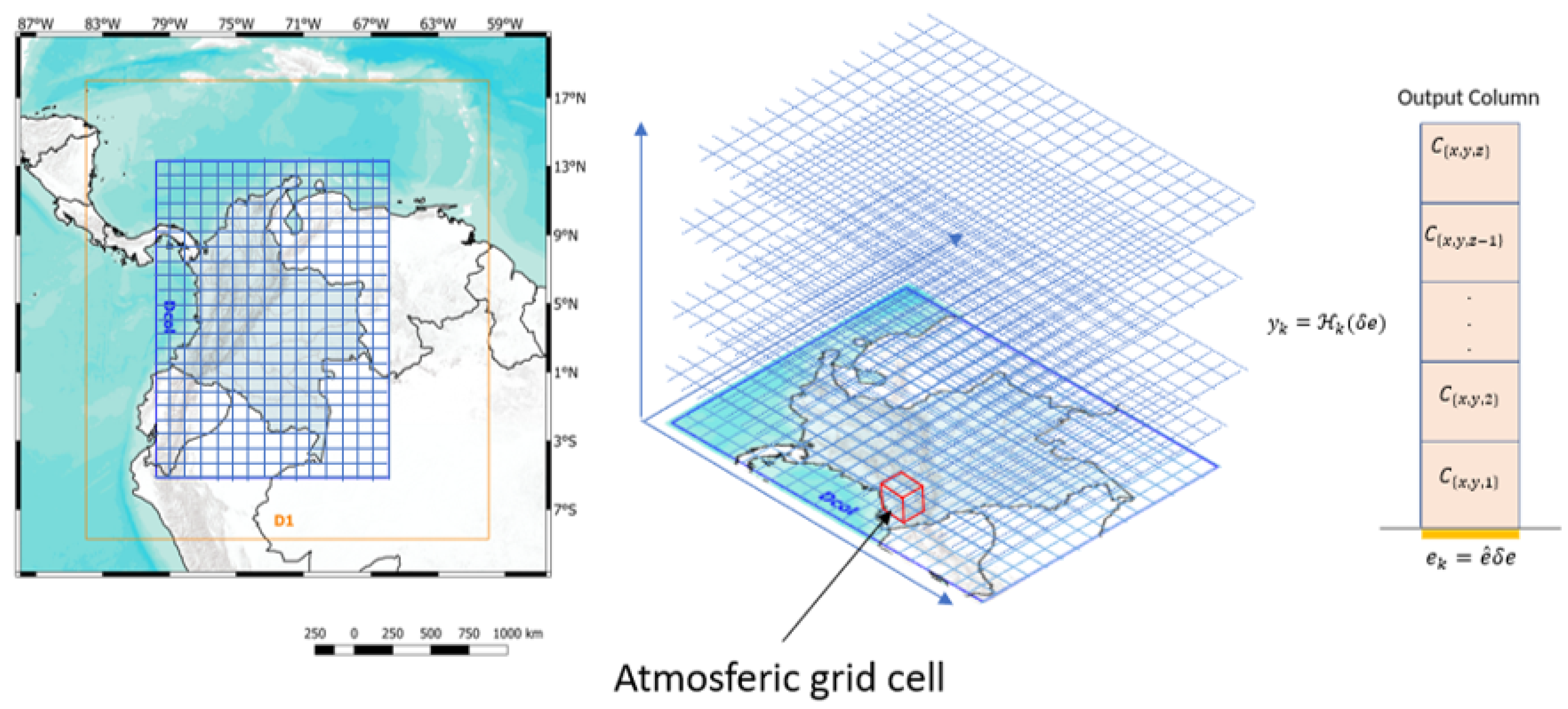
2.1. LOTOS-EUROS Simulations

LOTOS-EUROS was used to simulate the troposphere and study NO 2 dynamics. A nested two domain configuration was used (Figure 1) to increase the study resolution domain. Boundary conditions were obtained from CAMSIRA (CAMS Interim Re-Analysis [44]) for the outer (D1) domain at a 0.27 ° horizontal resolution with a size of (2957 km × 2668 km). The inner domain (Dcol), with a grid resolution of 0.09 ° (∼10 km) and with a extent of 1981 km × 1541 km, encompasses the continental Colombian territory, western Venezuela, almost all of continental Ecuador, the north of Peru and a small fraction of the Brazilian Amazon.
Table 1 summarises the simulation model settings. The meteorological input was obtained from the European Centre for Medium-Range Weather Forecasting (ECMWF) with a 0.07 deg ∼7.8 km of horizontal resolution and 18 levels of vertical resolution. We used updated land cover and topography data [45]. The topography was updated to the GTMED2010 global digital elevation model (Spat.res: 0.002 ° ), while land cover data were updated to the LCCCI2009 (Land cover from the Climate Change Initiative), on a resolution of 0.3 km × 0.3 km.
Due to the lack of a regionally detailed and updated emissions inventory, emissions input data were obtained from the Emission Database for Global Atmospheric Research (EDGAR v.4.3.2) (https://edgar.jrc.ec.europa.eu/, accessed in January 2019). Depositions were calculated using the DEPosition of Acidifying Compounds (DEPAC) module [46]. More details about the parametrisation of the model for this experiment can be found in Manders et al. [14]

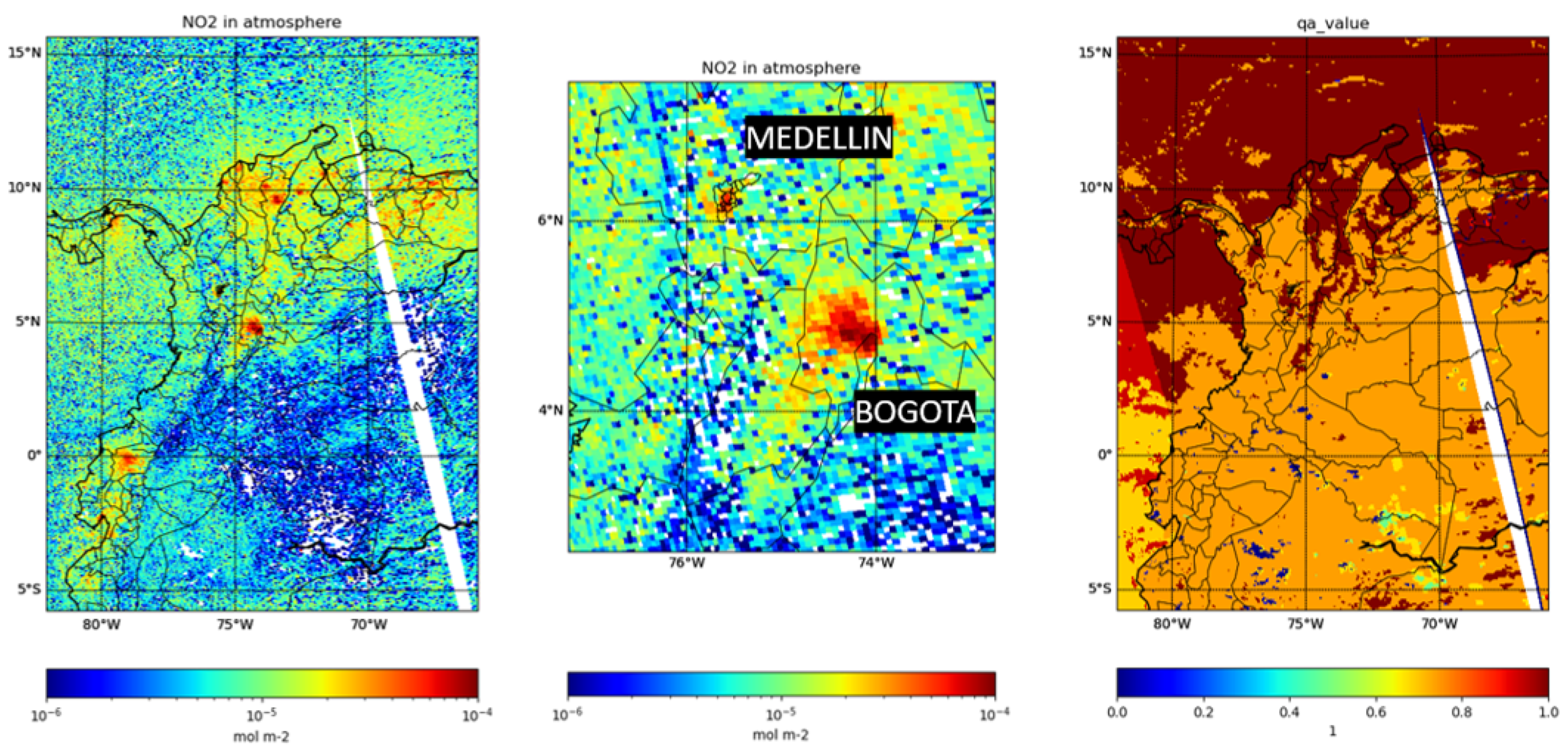
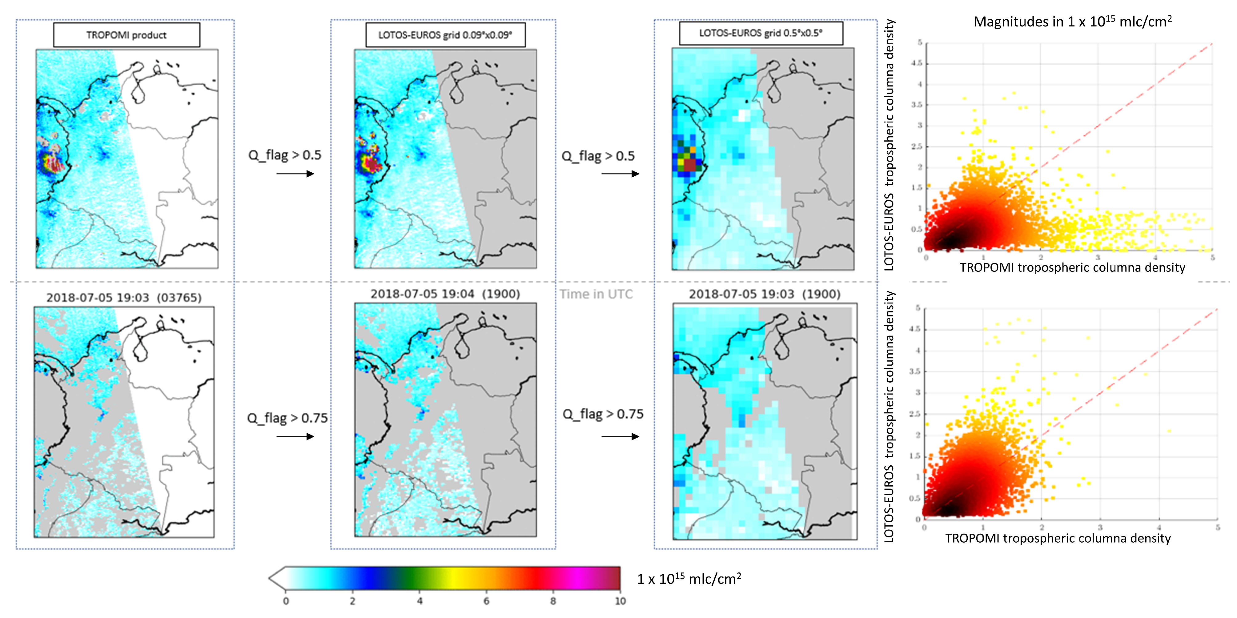
2.2. TROPOMI Satellite Data

NO 2 satellite data products were obtained from the TROPOMI TM5-MP/DOMINO offline data from (www.temis.nl) [47] and reprojected to the grid of the LOTOS-EUROS model ( 0.09 ° × 0.09 ° ) simulation to facilitate graphical comparison. Each grid cell was filled with a area-weighted sum of contributions from pixels that (partly) overlap the cell. A model simulation of the satellite retrieval could be derived from the multiplication of the average kernel with the satellite product concentration column of the LOTOS-EUROS concentration to produce simulations of the gridded data. The average kernel integrates the concentrations over height, as the sensitivity of the satellite instrument to tracer densities is height-dependent. The model profile is convoluted with these averaging kernels, provided in the satellite download data product to simulate the retrieval for a correct model and satellite retrieval products comparison [48]. The averaging kernels are implemented to the model output at the time of the nearest satellite overpass, which is usually at 18:30 UTC [49]. A selection on the pixel quality flag ( q a ) was been applied, averaging over the pixels filtered for ( q a ) > 0.55. This contrasts with [42] who recommend using pixels with a q a value of 0.52 or above for data assimilation and model comparison studies.
For data assimilation, it is essential to get estimations of the accuracy of the observations to construct the observation error covariance matrix, the error from the observations is used to construct a diagonal matrix R because the error values at this stage are correlated only with the observed state in the already remapped grid. The inaccuracies in the TROPOMI observations result from the retrieval method’s three stages that are a previous step in the preprocessing of the satellite information from manipulating the crude light spectroscopy data to have the NO 2 vertical column density. The stages that add errors in this process are the quantification of slant columns, the separation of the stratospheric and tropospheric components of slant columns, and the tropospheric air mass factors multiplication [42]. The overall error is provided per pixel in the TROPOMI data product.

2.3. Data for Validation

To validate the results, two sources of information were used: The first corresponded to version 4.0 of the Nitrogen Dioxide (NO 2 ) Standard Product (OMNO2) from the Ozone Monitoring Instrument (OMI) on board of the AURA satellite since 2004. OMI is the precursor of the TROPOMI instrument and the two NO 2 measurements have been compared previously [42,50]. In this work, OMI data were used to calculate the tropospheric NO 2 vertical column density (VCD) time-series, which can be found at (https://disc.gsfc.nasa.gov/datasets/OMNO2, data accessed in May 2021). The overpass time of the instrument is at 18:00 UTC also in a synchronous orbit. OMI’s spatial footprint is approximately 13 km by 24 km for the nadir pixels. Spatial resolution reduces as the swath edge approaches (pixel size rises). The second, consisted of data from the Sistema de Alerta Temprana del Valle de Aburrá (SIATA), a network of sensors that offer high-quality measurements for different pollutants in the atmosphere across the Aburrá Valley, monitoring species such as O 3 , SO 2 , PM 10 , PM 2.5 , and PM 1 . The network has seven ground-based sensing stations for NO 2 . SIATA data is available (https://siata.gov.co/descargasiata/index.php/index2/, data accessed in June 2021).

3. 4DEnVar Formulation

The 4DEnVar methodology is used for estimating uncertain parameters. In our application, the emissions are the major sources of uncertainty, and they are parameterised by introducing multiplicative correction factors. Let δ e n with n the number of uncertain parameters, represent the unknown LOTOS-EUROS emission correction factors. The emissions e k at time k are calculated according to
e k = e ^ k ( 1 + δ e )
with e ^ k as the nominal emissions at time k from the emission inventory.
We want to estimate the emission correction factors δ e using all the observations available. Let y k m with m the number of observations at time k, related to the parameters δ e via the nonlinear observation operator H k . This operator H k includes the LOTOS-EUROS model to relate the emission correction factors with the concentrations, and the satellite kernel to map the column concentrations to the retrieval satellite representation:
y k = H k ( δ e ) .
The correction factors δ e are estimated by the minimisation of a cost function. This is a function of the n unknown parameters over a time window defined from k = 0 to k = T that measures the differences between the satellite observations and the model representation of these observations:
J ( δ e ) = 1 2 δ e e b B 1 2 + 1 2 k = 0 T d k R 1 2 ,
where · is the L 2 norm, e b is the first guess of the emission correction factors, B is the n × n background error covariance matrix, R corresponds to the m × m observation error covariance matrix and d k is the innovation vector:
d k = y k H k ( δ e ) ,
The basic idea of the 4DEnVar method is to estimate the sensitivities of the observations with respect to changes in the parameters using directly the computation of the LOTOS-EUROS model instead of using its tangent linear model and its adjoint. This is done by generating an ensemble of forward model simulations that is used to obtain a linear approximation of the operator H k [1,51]. Perturbations of the parameters are used to create this ensemble. For the details of the methodology, the reader is referred to [36].
In ensemble-based data assimilation, the background covariance matrix B can be approximated by the ensemble sample covariance matrix
B = X b · X b T ,
with X b R n × N equal to
X b = 1 N 1 [ δ e ( 1 ) δ e ¯ , δ e ( 2 ) δ e ¯ , , δ e ( N ) δ e ¯ ] ,
where δ e ( i ) is the i-th emission correction factor ensemble member, δ e ¯ is the mean emission correction factor among all the ensembles, and N is the ensemble number.
The cost function (3) can be rewritten as a function of a new parameter δ X e n s using X b as Control Variable Transform (CVT):
δ e = X b δ X e n s
This idea is also known as the preconditioning step in optimisation problems (see in [36]). This method improves the conditioning of the optimisation problem.
The choice of the emission correction parameters to be estimated and the quantification of their uncertainty is critical in designing the assimilation system because this should reflect the most significant uncertainty of the CTM model. As chemical species can be sensitive to physical and chemical processes, the primary uncertainty source could differ depending on the species of interest.
In order to minimise (3), the gradient of the cost function is required. The expression for the gradient of the cost function in terms of the parameters δ X e n s can be shown to be [36]
J ( δ X e n s ) = δ X e n s + k = 0 T Y k T · R 1 · ( d k Y k · δ X e n s ) ,
where
Y k = H k · X b 1 N 1 ( H k ( δ e ( 1 ) ) ) y k ¯ , , ( H k ( δ e ( N ) ) ) y k ¯ .
and H k is the linear approximation of the observation operator H k . Once the gradient has been computed, the parameters can be improved using some gradient-based updating scheme. After a number of iterations, a new ensemble of model simulations can be generated using perturbations of the parameters around the latest estimate of these parameters, and these ensembles can then be used to approximate the observation operator more accurately.
For cases where the number of parameters is not too large, there is an alternative algorithm. By setting the gradient of the cost function equal to 0, the following system of equations for δ X e n s can be obtained:
( I k = 0 T Y k T · R 1 · Y k ) · δ X e n s = k = 0 T Y k T · R 1 · d k
δ X e n s can now be solved from this system of equations. This procedure can also be repeated, starting with the latest estimates of the parameters, by generating a new ensemble of model simulations through perturbing these parameters, and by computing a new linear approximation of the observation operator. For large scale problems, this implementation is not attractive from the computational point of view and a gradient-based minimisation algorithm based on Equation (8) is to be preferred. This is the implementation that has been used in this paper.
After the successive implementation of one of the techniques just described, the parameters δ e can finally be calculated using (7). The input to this procedure is the CTM model, the satellite observations, and the parametrisation of the algorithm (e.g., window length, inner loops and convergence criteria) and the output is the set of optimised parameters.
Figure 2 shows the setup of the 4DEnVar assimilation process proposed for the first days of February 2019, A simulation of 15 days over 16 January to 1 February was performed before data assimilation to identify the locations where emission parameters required improvement. Data assimilation was performed over individual days (2 and 3 February). Each assimilation was preceded by a 1-day spin-up period, where the simulated fields stabilised and became independent of the initial conditions. During assimilation, the observations (satellite data available from the TROPOMI instrument at 13:30 local time) were incorporated to estimate the value of the initial emission factor parameters. To find the proper parameters, the optimisation procedure consisted of an outer/inner loop iteration to reach the convergence criteria or the maximum number of iterations defined. The iteration procedure was terminated when the maximum iteration number was reached, or when the minimal error criteria was met.
To perform the assimilation window, the 4DEnVar weighted an ensemble of 40 model trajectories generated from perturbing the emission factor parameters, based on how much the ensemble matched the observations and the background state. From this, based on its minimisation procedure, a limit of 15 was set for the number of iterations for the inner loop of the 4DEnVar implementation step. Incorporating more than 15 iterations demonstrated no reduction of the cost function. The 4DEnVar result (known as analysis in many data assimilation scenarios) is the model value for the emission parameters updated in the previously chosen positions. The performance metrics used in this work are summarised in Appendix A.

4. Results and Discussion

This contribution assumes the problem of dealing not only with an under representation of the boundary conditions for modelling but also with the scarcity of data. Previous section addressed the model and the data assimilation technique. TROPOMI observations flag considerations are used to compare it appropriately with the simulations of the model. Afterwards the 4DEnVar TROPOMI assimilation uses the simulated columns for Nitrogen Dioxide and the vertical profiles comparison. The impact of the estimation over major cities in Colombia and the relationship between surface and satellite data is addressed looking for the proper establishment of the benefits of this technique.

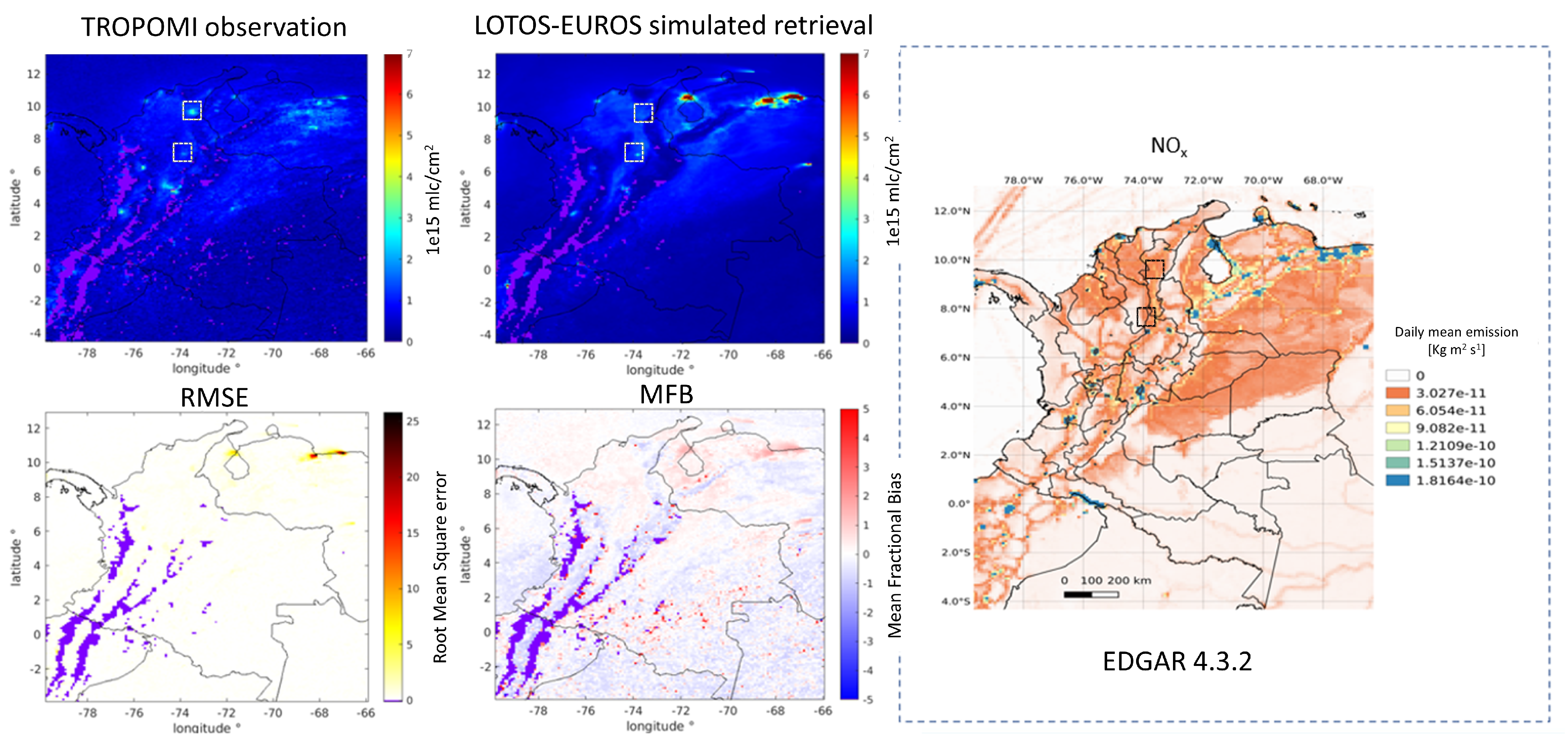
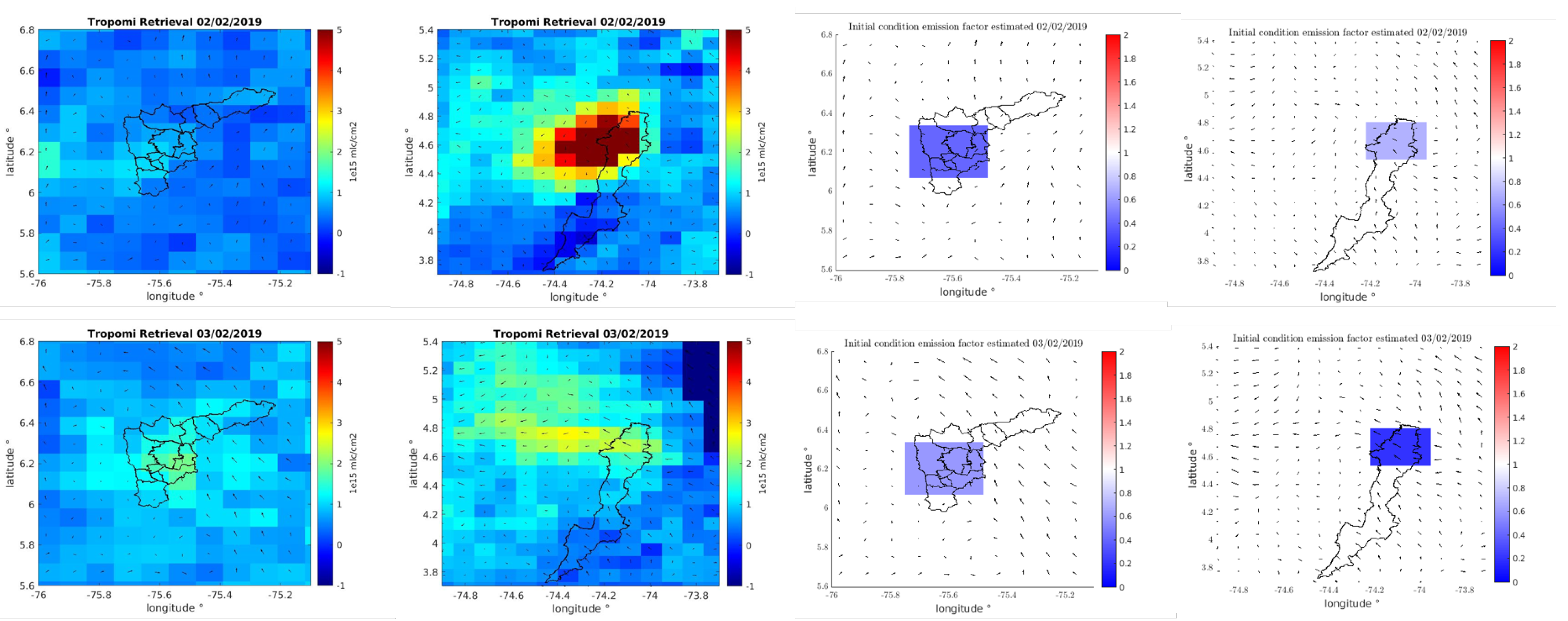
4.1. Comparison of TROPOMI Observations with LOTOS-EUROS Simulated NO 2 Column Concentration

Figure 3 shows an example of the regridded satellite data, presenting how the NO 2 footprint demarcates the principal Colombian cities. The right panel of this Figure shows an example of these quality flags q a values. A q a for the retrieval is provided for each pixel recovered, this number might be something between 0 and 1, which is mainly determined by the presence of clouds above the pixel. q a value > 0.75 cloud-covered scenes partially snow/ice covered scenes, errors, and problematic retrievals. q a value > 0.5 adds good-quality retrievals over clouds and over scenes covered with snow/ice, useful for assimilation and model comparison studies. For this comparison, the satellite quality flag was configured in 0.75 to avoid artefacts that do not necessarily correspond to NO 2 concentrations.
To see the effects due to the quality filter over this region, the Figure 4 shows the comparison of the TROPOMI output in the first left column, and the simulation kernel transformation for two different grid resolutions (0.09° and 0.5°) and the scatter plot between the tropospheric column density from the satellite and the LOTOS-EUROS simulated column density, showing a large divergence between the satellite simulated data and the output from the model.
A qualitative comparison of the simulated and observed NO 2 column densities was conducted to detect locations where the TROPOMI observations differed significantly from the LOTOS-EUROS simulations to focus the attention therein for the data assimilation emission estimation experiment. Figure 5 shows a comparison between the 15-day average satellite observations (16 January–February 2019) with the LOTOS-EUROS NO 2 column, as well as the EDGAR NO x emission inventory on the right image.
The NO 2 concentration in the model and the observations presented high values over the main urban centres, but the amplitude of the simulated NO 2 concentrations often differed. Simulated values over the densely populated area of Venezuela that includes Caracas, Valencia, Barquisimeto and Maracaibo (a region known as the oil refinery corridor) showed much higher values in the model simulation output than the satellite observations, and in consequence, showed the highest root mean square error (RMSE; lower-left in Figure 5). A Mean Fractional-bias (MFB; lower-centre in Figure 5) calculation showed a broader perspective over the domain, revealing that the model underestimated the NO 2 in the south except for some isolated, overestimated points over the southern Colombian Amazon. The model also underestimated NO 2 concentrations along the Magdalena River valley in the north of Colombia.

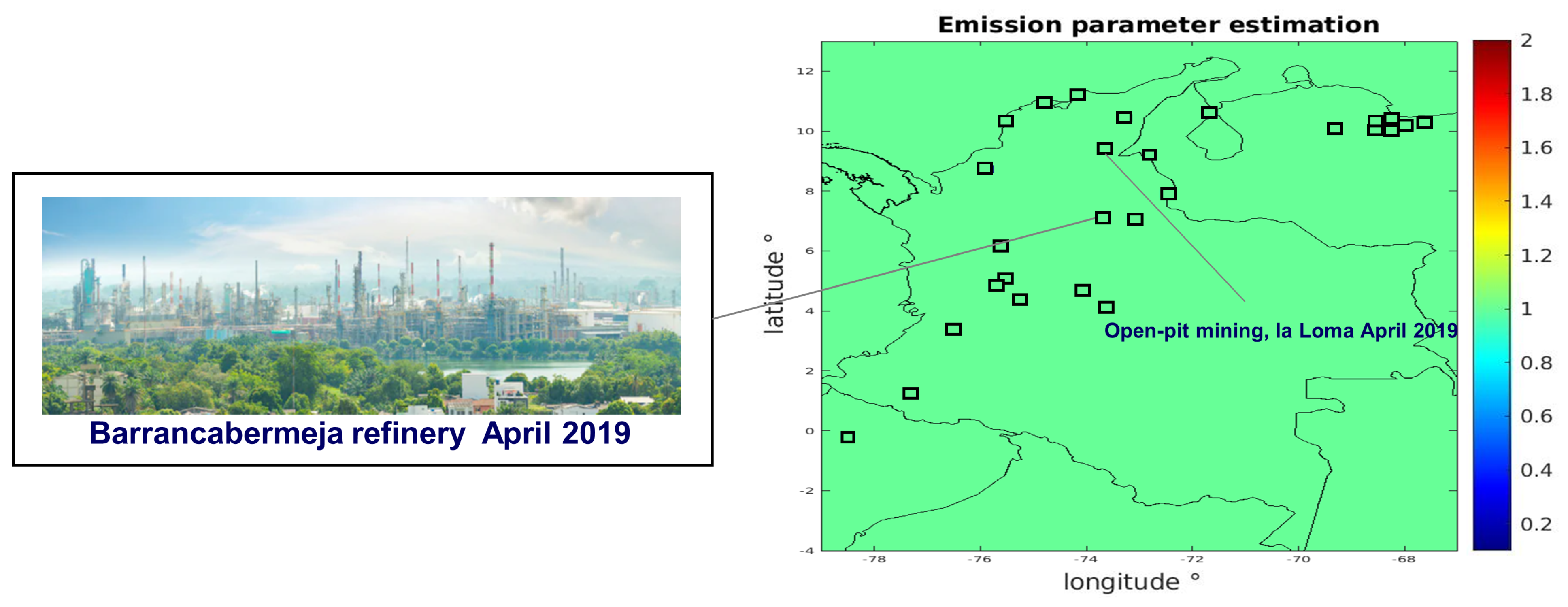
4.2. Parameter Location and Perturbation Model

The discrepancies between the LOTOS-EUROS model and the observations were mostly attributable to the uncertainty in model emission parameters [15,34]. For the region of interest, the inventories are not accurate, that is the reason why accurate emissions for specific components such as PM 2.5 were estimated recently for example for cities like Medellín using an EnKF DA technique [15], nevertheless for the coarse domain the inventories and other pollutants the emission inventories remain uncertain. Different perspectives have been taken into account for the emission parameter estimation problem using satellite information and data assimilation variational (4DVar) techniques ([52,53,54,55,56], and also from the sequential (EnKF, OI) techniques [57,58].
Twenty seven locations were selected for perturbing the model’s parameters in order to generate a subspace of model ensemble trajectories to estimate appropriate values driven by the observations; black squares in Figure 6 denote the areas selected over the initial nominal emission parameter value. These correspond not only to the major cities, but also to other areas of interest denoted in the previous Figure 5, one is the main oil refinery in Colombia located in the central part of the country in the Magdalena River valley and the other an open-pit coal mine mining in northern Colombia near the Venezuelan border that presented anomalous concentration values in a rural area. The emissions for these 27 locations were updated using the 4DEnVar data assimilation.
Each perturbation location consisted of a 3 × 3 buffer of 0.09° grid cells. The emission factor perturbation value multiply the concentrations homogeneously in the area where the estimation of the parameter was made. The reason for this buffer of 9 grids is that TROPOMI samples the downwind plume, which might be 1–2 grid cells away from the source.

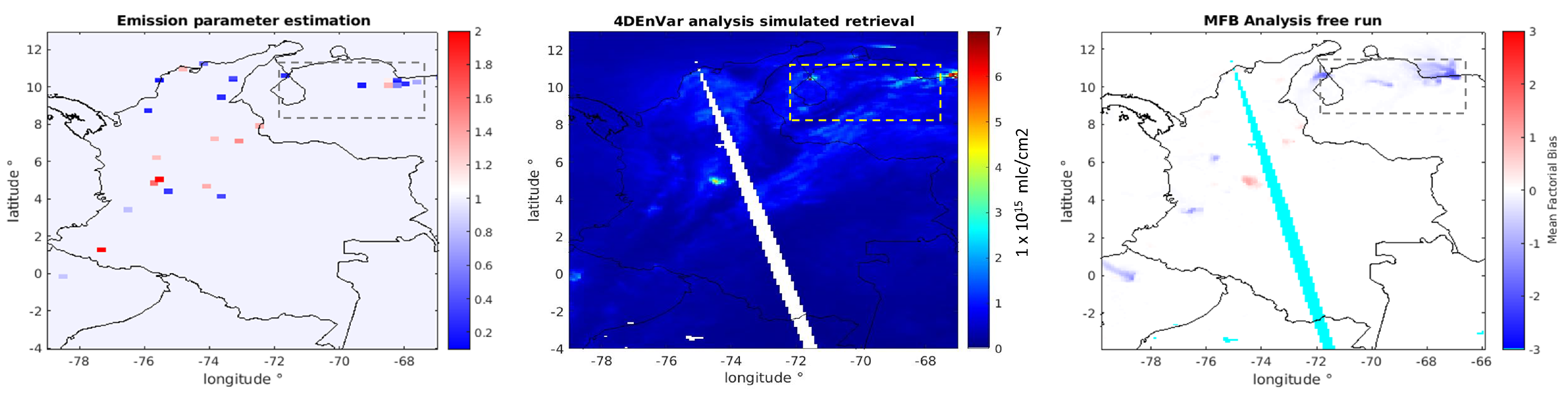
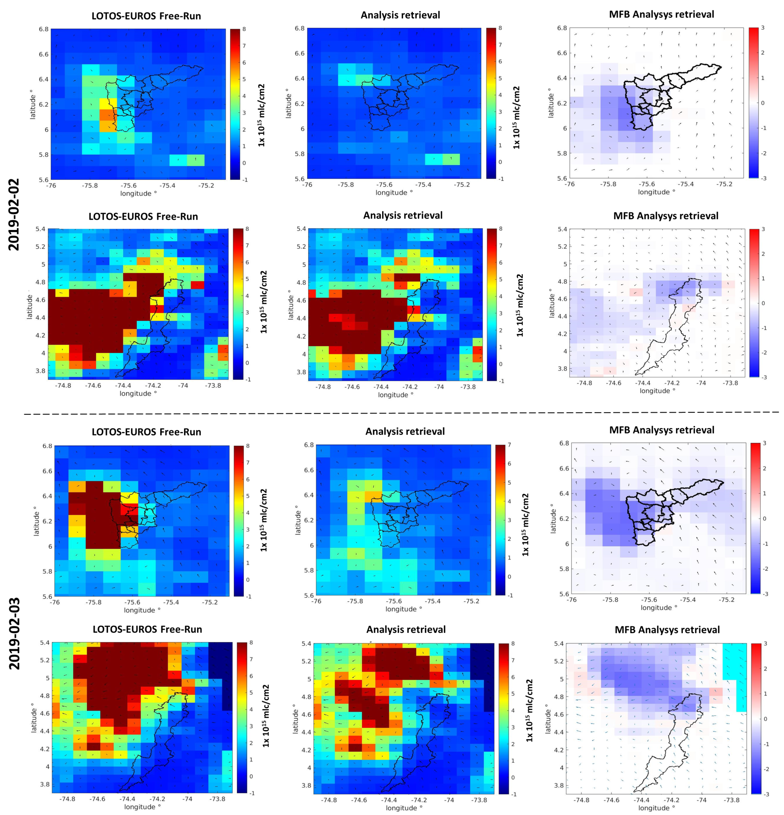
4.3. 4DEnVar LOTOS-EUROS Data Assimilation Using TROPOMI Data

4.3.1. Simulated NO 2 Columns

Figure 7 shows the NO 2 columns concentrations from the LOTOS-EUROS before assimilation (free run) and the TROPOMI retrieved product for the 2 of February 2019. Although the satellite data presented gaps (white areas) due to the quality filter, it was possible to observe a difference between the model simulation and the observation from the remote instrument. The dashed rectangle marks a relatively flat area in Venezuela where good quality observations, due to low cloud cover, are present and where the model overestimates the satellite product denoting areas to update the emission parameters. Other cities like Bogotá, Medellín, Barranquilla and Quito also present differences between LOTOS-EUROS and the satellite information. An open-pit mining operation in northeastern Colombia stands out in the satellite observations as a prominent NO 2 source point, as do small cities along the gulf of Maracaibo.
The left panel of Figure 8 shows the emission factors obtained with the 4DEnVar technique, showing the estimated values of the 27 emission parameters location selected based on the preliminary simulation over the domain. In the north part of the domain, mainly in the Venezuelan dashed area, adjustment factor values below 1 and overestimation of the model relative to the satellite observations. In some areas in the centre of Colombia, the region with the highest population density, the analyses suggest a model underestimation.
The 4DEnVar analysis output is shown in the centre mosaic in the Figure 8. This graphic shows the NO 2 column that the LOTOS-EUROS model simulated using the updated emission parameters. The image on the right shows the MFB between this analysis step and the background condition; here it is possible to appreciate the spatial over/underestimations between both scenarios resulting from the updated initial parameter values. The area’s values in the dashed square region in the previous Figure 6 needed to reconciliate the LOTOS-EUROS simulations with the TROPOMI observations, with values < 1 indicating LOTOS-EUROS over-estimations, and values > 1 indicating underestimations (observations > simulated values), suggest a reduction of (0.2–0.6) in some areas of interest. With the new emission factors, the emissions within the rectangle were strongly reduced, leading to simulated lower magnitude NO 2 columns in better agreement with the TROPOMI simulations. Curaçao shows a plume with a high east-west trend in the LOTOS-EUROS that is not appreciated in the TROPOMI data for this day and where we did not put an update emission. Is it possible to see in the analysis simulation how the same plume appears indicating that the model not was modified for this location. The value of the parameters and the comparison of the results is presented with the MFB in the right panel, using the emissions estimated to propagate a new forward run (4DEnVar analysis simulated retrieval) and the free run. Locations where the emission adjustment does not help presumably, are the locations where the satellite information is not complete, such as the Andean mountain corridor and regions for which the emission are too low in the current inventory and no matter the parameter estimated suggests changes, they are not evident.

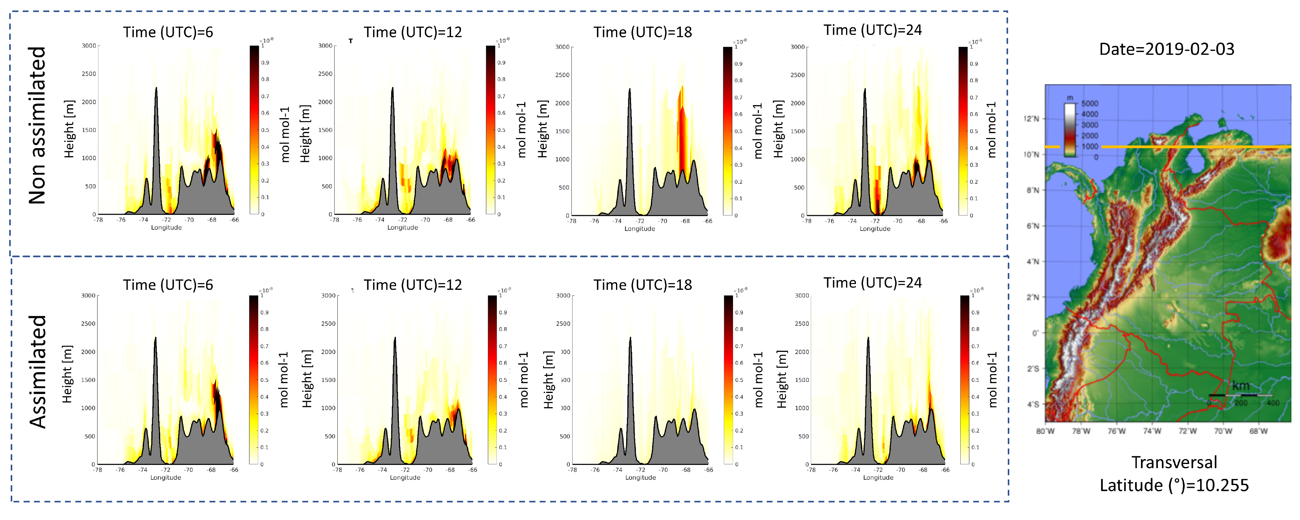
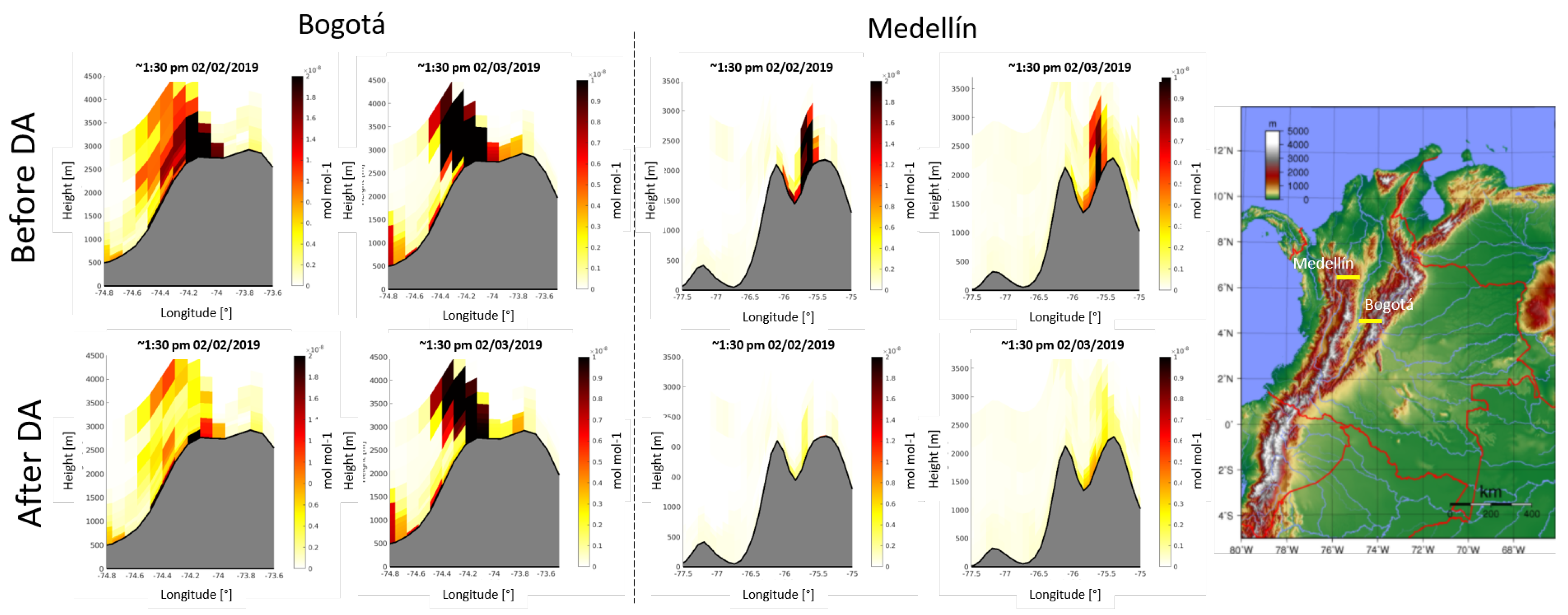
4.3.2. Vertical Profiles

Figure 9 shows a comparison between the assimilated and non-assimilated vertical NO 2 concentrations at latitude 10.255 ° for four different time steps (1 a.m., 7 a.m., 1 p.m., 7 p.m. UTC) during the second assimilation day (3 February 2019). This mosaic compares the changes in the vertical profiles of this gas. This latitude corresponds to the locations of the parameters with the highest emissions in Venezuela, originating in part from the high concentration of oil refineries in the area. The non-assimilated scenario displays a higher NO 2 concentration than the assimilated scenario, it is evident how the plume partially disappear for moments like at the 1 pm presumably due to the updating of emissions, which conditions the intensity of concentrations in subsequent hours. The emission was updated with the parameters estimated, suggesting for this location a decrease of the emissions for the current time for the experiment. These results could be explained by the fact that during the last ten years, there has been a dramatic reduction in oil production in Venezuela due to the U.S sanctions, with an accompanying decrease in refining activity [59]. The 2012 emission inventory used in this paper does not account for these geopolitical ramifications. With these findings, it is advised that the rate of emission for this area is adjusted based on the assimilation of satellite observations.

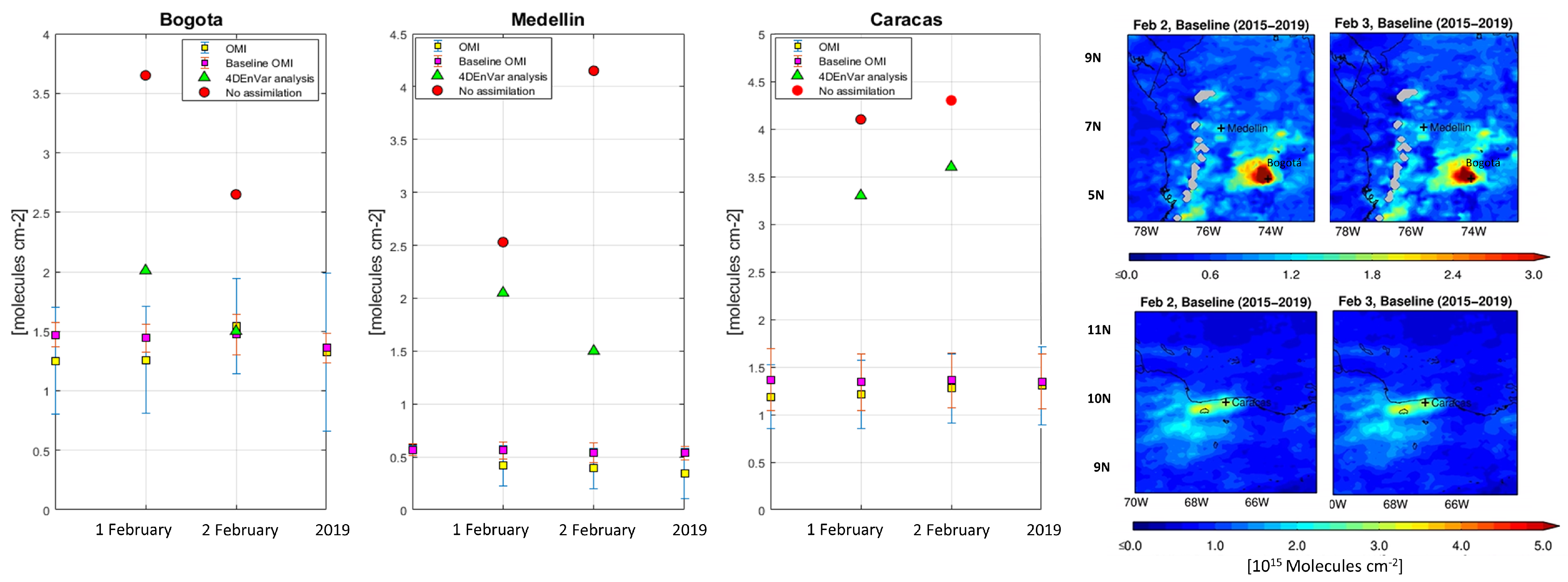
4.3.3. Impact over Major Cities

The 4DEnVar results have been evaluated in more detail for the cities of Medellín and Bogotá (Figure 10). In the corresponding close-ups it is also possible to appreciate the prevailing east-west 10 meter wind pattern comes from the ECMWF input wind fields interpolated at the LOTOS-EUROS simulation grids. The TROPOMI retrieval is shown in the two left columns, while the emission factors estimated are in the two right columns.
For the two assimilation days the change of the value of this new emission parameter from the nominal value has an impact on the concentration fields as shown in Figure 11. The second assimilation day integrates the emissions being estimated as the new nominal values to start the new assimilation window. Figure 11 shows the difference between the background NO 2 plumes and the retrieval with the estimated parameters. The 10 m wind fields from the LOTOS-EUROS model are shown in the figures as well as the concentration plumes. The magnitude reduction due to the emission update is shown for the assimilated scenario reducing spatially the concentration along the flow trajectory.
Figure 12 shows the vertical cross sections for the city of Bogotá and Medellín for the two assimilation days declared in the schematic of Figure 2 before assimilation and with data assimilation. Bogotá is located atop a high-altitude plateau where the prevailing NO 2 transport occurs from east to west. The assimilation effect is noticeable in terms of the magnitude of the concentration reduction in the plume transported in this direction. Medellín is located in a deep valley (Aburrá Valley). Here the assimilation effect is noticeable in terms of the magnitude of the concentration reduction inside the valley.

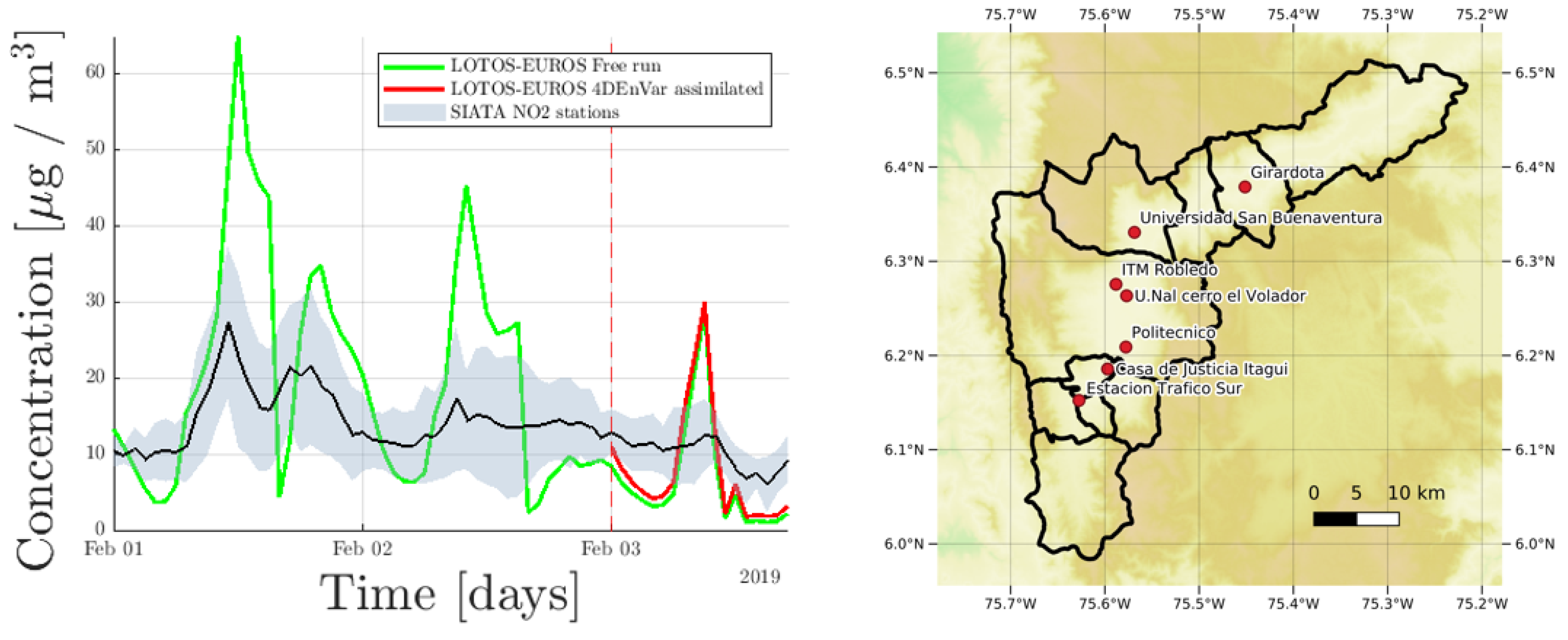
4.4. Comparison with SIATA Surface Observations and OMI Measurements

For the City of Medellín, surface measurements of NO 2 are available along the valley from the ground-based sensor network measurements from the Sistema de Alerta Temprana del Valle de Aburrá (SIATA; Figure 13), with stations located mainly at the bottom of the valley. The figure shows the mean of the concentration magnitude for all the available stations with their standard deviation spread against the non assimilated and 4DEnVar assimilated model output. The study period corresponds to one of comparatively low atmospheric loads for NO 2 .
Table 2 shows the MFB and RMSE and the Correlation factor comparison in the assimilation period for the free run and assimilated propagation against the mean of the observation network. For this location from the assimilation experiment, the estimated emission parameter suggests an increase in the emission value ( e > 1 ), which is appreciated in reducing the MFB and RMSE statistic and increasing the correlation factor.
For this area the comparison was not too relevant in modifying the initial conditions for the analysis value, because the TROPOMI information was not very significant for the experiment period to promote a drastic update in the parameters. At the same time, in Medellin’s vertical cut, the effect was more evident in the concentration of higher levels that was seen in Figure 11. It was possible to see how the analysis tends to search the mean value from the ground observation. No more NO 2 observations were available around the domain at the time of this study.
Comparisons were made against OMI measurements. Only data that were of excellent quality (VCD Quality Flags of 0) and cloud screened (Effective Cloud Fraction 30 percent) were included in the analyses. Figure 14 shows the OMI vertical column density, expressing the “baseline” concentrations as the weighted average of all daily values for 2015–2019. For all the cities, the magnitude of the concentration value simulated from the model decreased approaching to the OMI magnitude. Different works have studied the effect of assimilation of satellite retrieved NO 2 data on emissions or Surface concentrations in a global domain [57,60] pointing towards the ability to estimate emissions by assimilating satellite observations that are taken only once per day over one place concerning with the NO 2 atmospheric life time during different times of the year. On another side regional domain estimation studies like Skoulidou et al. [49], Wang et al. [61] orient our subsequent emission experiments toward the interest of persistent emission estimation capabilities.

5. Conclusions

A 4DEnVar methodology has been developed to combine TROPOMI satellite observations with LOTOS-EUROS regional CTM simulations for the northwest of South America. This paper shows the viability of this method in dealing with a small number of highly nonlinear reactive species such as NO 2 in a control scenario.
Cities and municipalities in developing countries without local air quality and meteorological networks can use this technique, that avoids the implementation of the adjoint of the CTM, to estimate coarse emissions inventories. In this study, emission correction factors defined as the uncertain parameters to be estimated multiply the nominal emission inventory.
Using the 4DEnVAR technique to assimilate the TROPOMI-NO 2 columns, the spatial and temporal concentration distribution of the NO 2 fields improves with the modification of those correction factors. The emission update has substantially enhanced the agreement between the simulated and observed NO 2 fields. These findings showed that TROPOMI NO 2 concentrations can be utilised to reconstruct spatial and temporal variable NO 2 components, making it relatively simple to enhance temporal NO 2 emission patterns in a forward modelling setting.
Although the satellite data have not yet been exploited for extended periods due to the high cloudiness, we have demonstrated how to use a 4DEnVAr data assimilation technique, and how we can take advantage of the relationships between observed and unobserved states of a chemical transport model to improve the model results. Adding satellite information to the model makes it possible to estimate a coarse emission inventory, which is also a good starting point for establishing higher resolution emission inventories or improving boundary conditions for high resolution nested simulations.
The particular results from this case study suggest a decrease in the emission values in notorious places like the refinery corridor in the Venezuela region, driven by the drastic decrease in oil production over the last ten years.
In the future, we will refine the surface information, complementing the region’s surface information with the satellite data and the meteorology from high resolution mesoscale models such as WRF, to represent more accurately patterns, like we see in deep-seated narrow valleys such as in Medellín. We will also improve the data assimilation methodology with the implementation of localisation techniques to reduce the well-known problems introduces by the use of a limited amount of ensembles.

Author Contributions

A.Y.B.: Conceptualisation, Methodology, Software, Writing—Original Draft. S.L.-R.: Methodology, Software. N.P.P.: Conceptualisation, Methodology, Writing—Review and Editing. O.L.Q.: Conceptualisation, Methodology, Writing—Review and Editing, Supervision. A.S.: Methodology, Software, Writing—Review and Editing. A.W.H.: Writing—Review and Editing, Supervision. All authors have read and agreed to the published version of the manuscript.

Funding

This research received no external funding.

Acknowledgments

The authors acknowledge the supercomputing resources available by the Centro de Computación Científica Apolo at Universidad EAFIT (http://www.eafit.edu.co/apolo, accessed in 3 December 2021) to conduct this work. TNO, TU Delft University, for their incomparable support. Acknowledges the unrestricted use of tropospheric NO 2 column data from the TROPOMI sensor from www.temis.nl, accessed in June 2019. Express acknowledges the ESA CCI Land Cover project to provide the updated land use for the study area to conduct this work. The authors gratefully acknowledge the Ministry of Science, Technology, and Innovation in Colombia (MinCiencias) for the financial support of Andrés Yarce Botero. Scholarship program No. 860-2019. The authors gratefully acknowledge Maria Juliana Yepes Burgos for the editing and English review.

Conflicts of Interest

The authors declare no conflict of interest.

Appendix A. Performance Metrics

The results have been evaluated using two different metrics to compare the simulations of the LOTOS-EUROS before and after assimilation with the validation data from the ground sensors.
The mean fractional bias (MFB) normalises the bias for each model–observation pair using division by the average of the model and observation before taking the sample mean:
M F B = 2 M k = 1 M y L E k y k o y L E k + y k o ,
The number of elements in the set is represented by M. The number of observations from all valid monitoring station data for the comparison time period of interest is M, the model simulation output is y L E i and the observation is y o i in this application. The MFB has a range of 2 to + 2 and has the benefit of preventing the bias from being dominated by a few high-value observations/simulation combinations in the case of substantial changes, such as those caused by a strong diurnal cycle [62].
The root mean square error (RMSE) represents the sample standard deviation of the differences between predicted values and observed values (Equation (A2)). The RMSE penalises a high variance, as it gives errors with larger absolute values more weight than errors with smaller absolute values [63]:
R M S E = 1 M k = 1 M y L E k y k o 2 .
The correlation coefficient depicts the relationship between the values of one data set (simulations) and the values of another data set (observations). A high number (approaching +1.0) indicates a strong direct link, while values around 0.5 indicate a moderate relationship and values below 0.3 indicate a weak relationship. A significant inverse association is indicated by a low negative value (approaching −1.0), whereas values near 0.0 suggest little, if any, relationship.
C o r r = k = 1 M H ( c ) k H ( c ) k ¯ ( y k y ¯ ) k = 1 M H ( c ) k H ( c ) k ¯ 2 k = 1 M ( y k y ¯ ) 2
where the overline denotes a sample mean over the M elements of the validation set.

References

  1. Carrassi, A.; Bocquet, M.; Bertino, L.; Evensen, G. Data assimilation in the geosciences: An overview of methods, issues, and perspectives. Wiley Interdiscip. Rev. Clim. Chang. 2018, 9, e535. [Google Scholar] [CrossRef] [Green Version]
  2. Sandu, A.; Constantinescu, E.M.; Liao, W.; Carmichael, G.R.; Chai, T.; Seinfeld, J.H.; Dăescu, D. Ensemble–Based data assimilation for atmospheric chemical transport models. In Proceedings of the International Conference on Computational Science, Singapore, 9–12 May 2005; Springer: Berlin/Heidelberg, Germany, 2005; pp. 648–655. [Google Scholar]
  3. Aleksankina, K.; Reis, S.; Vieno, M.; Heal, M.R. Advanced methods for uncertainty assessment and global sensitivity analysis of an Eulerian atmospheric chemistry transport model. Atmos. Chem. Phys. 2019, 19, 2881–2898. [Google Scholar] [CrossRef] [Green Version]
  4. Aleksankina, K.; Heal, M.R.; Dore, A.J.; Oijen, M.V.; Reis, S. Global sensitivity and uncertainty analysis of an atmospheric chemistry transport model: The FRAME model (version 9.15. 0) as a case study. Geosci. Model Dev. 2018, 11, 1653–1664. [Google Scholar] [CrossRef] [Green Version]
  5. Mallet, V.; Sportisse, B. Uncertainty in a chemistry-transport model due to physical parameterizations and numerical approximations: An ensemble approach applied to ozone modeling. J. Geophys. Res. Atmos. 2006, 111, 118751. [Google Scholar] [CrossRef]
  6. Guevara, M.; Lopez-Aparicio, S.; Cuvelier, C.; Tarrason, L.; Clappier, A.; Thunis, P. A benchmarking tool to screen and compare bottom-up and top-down atmospheric emission inventories. Air Qual. Atmos. Health 2017, 10, 627–642. [Google Scholar] [CrossRef] [Green Version]
  7. Pachón, J.E.; Galvis, B.; Lombana, O.; Carmona, L.G.; Fajardo, S.; Rincón, A.; Meneses, S.; Chaparro, R.; Nedbor-Gross, R.; Henderson, B. Development and evaluation of a comprehensive atmospheric emission inventory for air quality modeling in the megacity of Bogotá. Atmosphere 2018, 9, 49. [Google Scholar] [CrossRef] [Green Version]
  8. Liu, F.; van der A, R.J.; Eskes, H.; Ding, J.; Mijling, B. Evaluation of modeling NO2 concentrations driven by satellite-derived and bottom-up emission inventories using in situ measurements over China. Atmos. Chem. Phys. 2018, 18, 4171–4186. [Google Scholar] [CrossRef] [Green Version]
  9. Kuenen, J.; Visschedijk, A.; Jozwicka, M.; Denier Van Der Gon, H. TNO-MACC_II emission inventory; a multi-year (2003–2009) consistent high-resolution European emission inventory for air quality modelling. Atmos. Chem. Phys. 2014, 14, 10963–10976. [Google Scholar] [CrossRef] [Green Version]
  10. Guevara, M.; Jorba, O.; Tena, C.; Denier van der Gon, H.; Kuenen, J.; Elguindi, N.; Darras, S.; Granier, C.; Pérez García-Pando, C. Copernicus Atmosphere Monitoring Service TEMPOral profiles (CAMS-TEMPO): Global and European emission temporal profile maps for atmospheric chemistry modelling. Earth Syst. Sci. Data 2021, 13, 367–404. [Google Scholar] [CrossRef]
  11. Timmermans, R.; Kranenburg, R.; Manders, A.; Hendriks, C.; Segers, A.; Dammers, E.; Zhang, Q.; Wang, L.; Liu, Z.; Zeng, L.; et al. Source apportionment of PM2. 5 across China using LOTOS-EUROS. Atmos. Environ. 2017, 164, 370–386. [Google Scholar] [CrossRef]
  12. Thürkow, M.; Kirchner, I.; Kranenburg, R.; Timmermans, R.; Schaap, M. A multi-meteorological comparison for episodes of PM10 concentrations in the Berlin agglomeration area in Germany with the LOTOS-EUROS CTM. Atmos. Environ. 2021, 244, 117946. [Google Scholar] [CrossRef]
  13. Schaap, M.; Timmermans, R.M.; Roemer, M.; Boersen, G.; Builtjes, P.; Sauter, F.; Velders, G.; Beck, J. The LOTOS? EUROS model: Description, validation and latest developments. Int. J. Environ. Pollut. 2008, 32, 270–290. [Google Scholar] [CrossRef]
  14. Manders, A.M.; Builtjes, P.J.; Curier, L.; Denier van der Gon, H.A.; Hendriks, C.; Jonkers, S.; Kranenburg, R.; Kuenen, J.J.; Segers, A.J.; Timmermans, R.; et al. Curriculum vitae of the LOTOS–EUROS (v2. 0) chemistry transport model. Geosci. Model Dev. 2017, 10, 4145–4173. [Google Scholar] [CrossRef] [Green Version]
  15. Lopez-Restrepo, S.; Yarce, A.; Pinel, N.; Quintero, O.; Segers, A.; Heemink, A. Forecasting PM10 and PM2.5 in the Aburrá Valley (Medellín, Colombia) via EnKF based data assimilation. Atmos. Environ. 2020, 232, 117507. [Google Scholar] [CrossRef]
  16. Casallas, A.; Celis, N.; Ferro, C.; Barrera, E.L.; Peña, C.; Corredor, J.; Segura, M.B. Validation of PM10 and PM2.5 early alert in Bogotá, Colombia, through the modeling software WRF-CHEM. Environ. Sci. Pollut. Res. 2020, 27, 35930–35940. [Google Scholar] [CrossRef] [PubMed]
  17. Henao, J.J.; Mejía, J.F.; Rendón, A.M.; Salazar, J.F. Sub-kilometer dispersion simulation of a CO tracer for an inter-Andean urban valley. Atmos. Pollut. Res. 2020, 11, 928–945. [Google Scholar] [CrossRef]
  18. Barten, J.G.M.; Ganzeveld, L.N.; Visser, A.J.; Jiménez, R.; Krol, M.C. Evaluation of nitrogen oxides sources and sinks and ozone production in Colombia and surrounding areas. Atmos. Chem. Phys. Discuss. 2019, 2019, 1–30. [Google Scholar] [CrossRef]
  19. Grajales, J.F.; Baquero-Bernal, A. Inference of surface concentrations of nitrogen dioxide (NO2) in Colombia from tropospheric columns of the ozone measurement instrument (OMI). Atmósfera 2014, 27, 193–214. [Google Scholar] [CrossRef] [Green Version]
  20. Quintero Montoya, O.L.; Niño-Ruiz, E.D.; Pinel, N. On the mathematical modelling and data assimilation for air pollution assessment in the Tropical Andes. Environ. Sci. Pollut. Res. 2020, 27, 35993–36012. [Google Scholar] [CrossRef] [PubMed]
  21. Bocquet, M.; Elbern, H.; Eskes, H.; Hirtl, M.; Žabkar, R.; Carmichael, G.; Flemming, J.; Inness, A.; Pagowski, M.; Pérez Camaño, J.; et al. Data assimilation in atmospheric chemistry models: Current status and future prospects for coupled chemistry meteorology models. Atmos. Chem. Phys. 2015, 15, 5325–5358. [Google Scholar] [CrossRef] [Green Version]
  22. Constantinescu, E.M.; Sandu, A.; Chai, T.; Carmichael, G.R. Ensemble-based chemical data assimilation. I: General approach. Q. J. R. Meteorol. Soc. A J. Atmos. Sci. Appl. Meteorol. Phys. Oceanogr. 2007, 133, 1229–1243. [Google Scholar] [CrossRef]
  23. Houtekamer, P.L.; Mitchell, H.L.; Pellerin, G.; Buehner, M.; Charron, M.; Spacek, L.; Hansen, B. Atmospheric data assimilation with an ensemble Kalman filter: Results with real observations. Mon. Weather Rev. 2005, 133, 604–620. [Google Scholar] [CrossRef] [Green Version]
  24. Houtekamer, P.L.; Zhang, F. Review of the ensemble Kalman filter for atmospheric data assimilation. Mon. Weather Rev. 2016, 144, 4489–4532. [Google Scholar] [CrossRef]
  25. Evensen, G. The Ensemble Kalman Filter: Theoretical formulation and practical implementation. Ocean Dyn. 2003, 53, 343–367. [Google Scholar] [CrossRef]
  26. Lorenc, A.C.; Jardak, M. A comparison of hybrid variational data assimilation methods for global NWP. Q. J. R. Meteorol. Soc. 2018, 144, 2748–2760. [Google Scholar] [CrossRef]
  27. Emili, E.; Gürol, S.; Cariolle, D. Accounting for model error in air quality forecasts: An application of 4DEnVar to the assimilation of atmospheric composition using QG-Chem 1.0. Geosci. Model Dev. 2016, 9, 3933. [Google Scholar] [CrossRef] [Green Version]
  28. Curier, R.; Timmermans, R.; Calabretta-Jongen, S.; Eskes, H.; Segers, A.; Swart, D.; Schaap, M. Improving ozone forecasts over Europe by synergistic use of the LOTOS-EUROS chemical transport model and in-situ measurements. Atmos. Environ. 2012, 60, 217–226. [Google Scholar] [CrossRef]
  29. Eskes, H.; Curier, L.; Segers, A. Assimilation of surface and satellite observations with the Lotos-Euros air quality model and the ensemble Kalman filter technique. In Proceedings of the EGU General Assembly 2012, Vienna, Austria, 22–27 April 2012; p. 12805. [Google Scholar]
  30. Barbu, A.; Segers, A.; Schaap, M.; Heemink, A.; Builtjes, P. A multi-component data assimilation experiment directed to sulphur dioxide and sulphate over Europe. Atmos. Environ. 2009, 43, 1622–1631. [Google Scholar] [CrossRef]
  31. Pinel, N.; Salazar, J.; Jose, P.; Rendon, A.; Quintero, O.; Yarce, A. Potential urban pollution impacts on protected areas in Colombia through atmospheric teleconnections. In Proceedings of the CMAS Community Modeling and Analysis system, Chapel Hill, NC, USA, 23–25 October 2017; pp. 3–5. [Google Scholar]
  32. Fu, G.; Heemink, A.; Lu, S.; Segers, A.; Weber, K.; Lin, H.X. Model-based aviation advice on distal volcanic ash clouds by assimilating aircraft in situ measurements. Atmos. Chem. Phys. 2016, 16, 9189–9200. [Google Scholar] [CrossRef] [Green Version]
  33. Lu, S.; Lin, H.; Heemink, A.; Fu, G.; Segers, A. Estimation of volcanic ash emissions using trajectory-based 4D-Var data assimilation. Mon. Weather Rev. 2016, 144, 575–589. [Google Scholar] [CrossRef] [Green Version]
  34. Jin, J.; Lin, H.X.; Heemink, A.; Segers, A. Spatially varying parameter estimation for dust emissions using reduced-tangent-linearization 4DVar. Atmos. Environ. 2018, 187, 358–373. [Google Scholar] [CrossRef]
  35. Liu, C.; Xiao, Q.; Wang, B. An ensemble-based four-dimensional variational data assimilation scheme. Part I: Technical formulation and preliminary test. Mon. Weather Rev. 2008, 136, 3363–3373. [Google Scholar] [CrossRef] [Green Version]
  36. Bannister, R. A review of operational methods of variational and ensemble-variational data assimilation. Q. J. R. Meteorol. Soc. 2017, 143, 607–633. [Google Scholar] [CrossRef] [Green Version]
  37. Burrows, J.P.; Weber, M.; Buchwitz, M.; Rozanov, V.; Ladstätter-Weißenmayer, A.; Richter, A.; DeBeek, R.; Hoogen, R.; Bramstedt, K.; Eichmann, K.U.; et al. The global ozone monitoring experiment (GOME): Mission concept and first scientific results. J. Atmos. Sci. 1999, 56, 151–175. [Google Scholar] [CrossRef]
  38. Flynn, L.; Long, C.; Wu, X.; Evans, R.; Beck, C.; Petropavlovskikh, I.; McConville, G.; Yu, W.; Zhang, Z.; Niu, J.; et al. Performance of the ozone mapping and profiler suite (OMPS) products. J. Geophys. Res. Atmos. 2014, 119, 6181–6195. [Google Scholar] [CrossRef]
  39. Bovensmann, H.; Burrows, J.; Buchwitz, M.; Frerick, J.; Noël, S.; Rozanov, V.; Chance, K.; Goede, A. SCIAMACHY: Mission objectives and measurement modes. J. Atmos. Sci. 1999, 56, 127–150. [Google Scholar] [CrossRef] [Green Version]
  40. Levelt, P.F.; van den Oord, G.H.; Dobber, M.R.; Malkki, A.; Visser, H.; de Vries, J.; Stammes, P.; Lundell, J.O.; Saari, H. The ozone monitoring instrument. IEEE Trans. Geosci. Remote Sens. 2006, 44, 1093–1101. [Google Scholar] [CrossRef]
  41. Veefkind, J.; Aben, I.; McMullan, K.; Förster, H.; De Vries, J.; Otter, G.; Claas, J.; Eskes, H.; De Haan, J.; Kleipool, Q.; et al. TROPOMI on the ESA Sentinel-5 Precursor: A GMES mission for global observations of the atmospheric composition for climate, air quality and ozone layer applications. Remote Sens. Environ. 2012, 120, 70–83. [Google Scholar] [CrossRef]
  42. Van Geffen, J.; Boersma, K.F.; Eskes, H.; Sneep, M.; Ter Linden, M.; Zara, M.; Veefkind, J.P. S5P TROPOMI NO2 slant column retrieval: Method, stability, uncertainties and comparisons with OMI. Atmos. Meas. Tech. 2020, 13, 1315–1335. [Google Scholar] [CrossRef] [Green Version]
  43. van der A, R.; de Laat, J.; Eskes, H.; Ding, J. Connecting the dots: NOx emissions along a West Siberian natural gas pipeline. In Proceedings of the EGU General Assembly Conference Abstracts, Online, 4–8 May 2020; p. 7633. [Google Scholar]
  44. Inness, A.; Ades, M.; Agusti-Panareda, A.; Barré, J.; Benedictow, A.; Blechschmidt, A.M.; Dominguez, J.J.; Engelen, R.; Eskes, H.; Flemming, J.; et al. The CAMS reanalysis of atmospheric composition. Atmos. Chem. Phys. 2019, 19, 3515–3556. [Google Scholar] [CrossRef] [Green Version]
  45. Yarce, A.B.; Montoya, O.L.Q.; Lopez-Restrepo, S.; Pinel, N.; Hinestroza, J.E.; Niño-Ruiz, E.D.; Flórez, J.A.; Rendón, A.M.; Alvarez-Laínez, M.L.; Zapata-Gonzalez, A.H.; et al. Medellin Air Quality Initiative (MAUI); Intechopen: London, UK, 2021. [Google Scholar]
  46. Van Zanten, M.; Sauter, F.; RJ, W.K.; Van Jaarsveld, J.; Van Pul, W. Description of the DEPAC Module: Dry Deposition Modelling with DEPAC_GCN2010; RIVM rapport 680180001; Rijksinstituut voor Volksgezondheid en Milieu RIVM: Utrecht, The Netherlands, 2010.
  47. van Geffen, J.H.G.M.; Eskes, H.J.; Boersma, K.B.; Veefkind, J. TROPOMI ATBD of the Total and Tropospheric NO2 Data Products; Report S5P-KNMI-L2-0005-RP; Royal Netherlands Meteorological Institute (KNMI): De Bilt, The Netherlands, 2021. [Google Scholar]
  48. Eskes, H.; Boersma, K. Averaging kernels for DOAS total-column satellite retrievals. Atmos. Chem. Phys. 2003, 3, 1285–1291. [Google Scholar] [CrossRef] [Green Version]
  49. Skoulidou, I.; Koukouli, M.E.; Segers, A.; Manders, A.; Balis, D.; Stavrakou, T.; van Geffen, J.; Eskes, H. Changes in Power Plant NOx Emissions over Northwest Greece Using a Data Assimilation Technique. Atmosphere 2021, 12, 900. [Google Scholar] [CrossRef]
  50. Wang, C.; Wang, T.; Wang, P.; Rakitin, V. Comparison and Validation of TROPOMI and OMI NO2 Observations over China. Atmosphere 2020, 11, 636. [Google Scholar] [CrossRef]
  51. Skamarock, W.; Klemp, J.; Dudhia, J.; Gill, D.; Liu, Z.; Berner, J.; Wang, W.; Powers, J.; Duda, M.; Barker, D.; et al. A Description of the Advanced Research WRF Model Version 4 (No. NCAR/TN-556+ STR); National Center for Atmospheric Research: Boulder, CO, USA, 2019. [Google Scholar]
  52. Kurokawa, J.I.; Yumimoto, K.; Uno, I.; Ohara, T. Adjoint inverse modeling of NOx emissions over eastern China using satellite observations of NO2 vertical column densities. Atmos. Environ. 2009, 43, 1878–1887. [Google Scholar] [CrossRef]
  53. Chai, T.; Carmichael, G.R.; Tang, Y.; Sandu, A.; Heckel, A.; Richter, A.; Burrows, J.P. Regional NOx emission inversion through a four-dimensional variational approach using SCIAMACHY tropospheric NO2 column observations. Atmos. Environ. 2009, 43, 5046–5055. [Google Scholar] [CrossRef]
  54. Zijlker, T. Estimating NOx Emissions Using S5-P TROPOMI: An Adjoint-Free 4DVAR Approach. Master’s Thesis, TuDelft University, Delft, The Netherlands, 2020. [Google Scholar]
  55. Wang, Y.; Wang, J.; Xu, X.; Henze, D.K.; Qu, Z.; Yang, K. Inverse modeling of SO2 and NOx emissions over China using multisensor satellite data—Part 1: Formulation and sensitivity analysis. Atmos. Chem. Phys. 2020, 20, 6631–6650. [Google Scholar] [CrossRef]
  56. Cooper, M.J.; Martin, R.V.; Henze, D.K.; Jones, D. Effects of a priori profile shape assumptions on comparisons between satellite NO2 columns and model simulations. Atmos. Chem. Phys. 2020, 20, 7231–7241. [Google Scholar] [CrossRef]
  57. Miyazaki, K.; Eskes, H.; Sudo, K. Global NOx emission estimates derived from an assimilation of OMI tropospheric NO2 columns. Atmos. Chem. Phys. 2012, 12, 2263–2288. [Google Scholar] [CrossRef] [Green Version]
  58. Ma, C.; Wang, T.; Mizzi, A.P.; Anderson, J.L.; Zhuang, B.; Xie, M.; Wu, R. Multiconstituent data assimilation with WRF-Chem/DART: Potential for adjusting anthropogenic emissions and improving air quality forecasts over eastern China. J. Geophys. Res. Atmos. 2019, 124, 7393–7412. [Google Scholar] [CrossRef]
  59. Su, C.W.; Khan, K.; Tao, R.; Umar, M. A review of resource curse burden on inflation in Venezuela. Energy 2020, 204, 117925. [Google Scholar] [CrossRef]
  60. Inness, A.; Baier, F.; Benedetti, A.; Bouarar, I.; Chabrillat, S.; Clark, H.; Clerbaux, C.; Coheur, P.; Engelen, R.; Errera, Q.; et al. The MACC reanalysis: An 8 yr data set of atmospheric composition. Atmos. Chem. Phys. 2013, 13, 4073–4109. [Google Scholar] [CrossRef] [Green Version]
  61. Wang, X.; Mallet, V.; Berroir, J.P.; Herlin, I. Assimilation of OMI NO2 retrievals into a regional chemistry-transport model for improving air quality forecasts over Europe. Atmos. Environ. 2011, 45, 485–492. [Google Scholar] [CrossRef]
  62. Boylan, J.W.; Russell, A.G. PM and light extinction model performance metrics, goals, and criteria for three-dimensional air quality models. Atmos. Environ. 2006, 40, 4946–4959. [Google Scholar] [CrossRef]
  63. Chai, T.; Draxler, R.R. Root mean square error (RMSE) or mean absolute error (MAE): Arguments against avoiding RMSE in the literature. Geosci. Model Dev. 2014, 7, 1247–1250. [Google Scholar] [CrossRef] [Green Version]
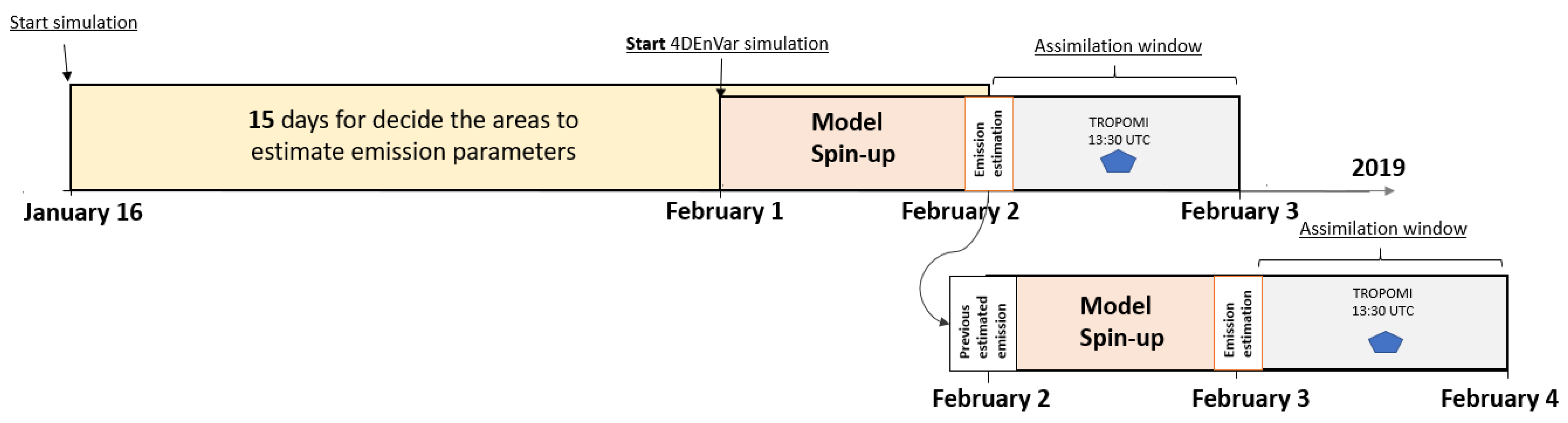
Figure 1. Illustration of simulation domains and vertical extent. (Left) Simulation nested domains. (Right) A conceptual state representation in the gridded model and the column being sampled by the observation operator that maps the emission parameters to the observation space H k ( δ e ) (see Section 3).
Atmosphere 12 01633 g001
Figure 2. Data assimilation (4DEnVar) procedure for emission parameter estimation. Simulations were run for 15 days (16–31 January) prior to the start of the data assimilation process. In the window 1–3 February, the ensemble was propagated without assimilation and in this new ensemble space the assimilation was performed for 2–3 and 3–4 February.
Atmosphere 12 01633 g002
Figure 3. TROPOMI NO 2 column measurements. (Right) TROPOMI Offline level 2 data for the overpass over Colombia on 2 April 2019. (Center) As before, zoomed over Bogotá and Medellí, the two largest (population-wise) Colombian cities. (Right) Quality flag values for the corresponding data.
Atmosphere 12 01633 g003
Figure 4. Illustration of the TROPOMI data downloaded before the re-gridding. (Upper) Data filtering at quality flag threshold of 0.5. (Lower), data filtering at quality flag threshold of 0.75. (Left column panels) TROPOMI data retrievals for the two qualitiy flags. (Center) TROPOMI data projected to LOTOS-EUROS grids at resolutions of 0.09 ° (center) or 0.5 ° (center-right). (Right) Scatter plots at comparing TROPOMI vs. LOTOS-EUROS pixel values for the resolution of 0.09 ° ).
Atmosphere 12 01633 g004
Figure 5. (Top left and centre) Fifteen days mean (16 January–1 February 2019) of the TROPOMI tropospheric NO 2 vertical column and the corresponding LOTOS-EUROS simulations. Purple areas correspond to areas where no data was available, mainly due to the cloudiness presence over the area for all that time. The dashed yellow squares correspond to two locations selected to update emissions that are not principal cities but considerable concentration spots seeing from the remote sensing instrument to qualitatively detect the right place to estimate unknown or uncertain parameters. (Bottom left and centre), root mean square error and modified-fractional-bias between retrieval and simulation. (Right), EDGAR V4.3.2 anthropogenic NO x emissions, 2012.
Atmosphere 12 01633 g005
Figure 6. Locations selected for emission parameter adjustment via 4DEnVar data assimilation. The 27 locations indicated in the (right) panel, corresponding primarily to large urban centres, were chosen for parameter adjustment based on the magnitude of the differences observed in Figure 5. (Left) Location of Colombia’s largest oil refinery (near the city of Barrancabermeja). The Drummond open-pit coal mine, a non-urban site whose emissions were poorly represented by the default emissions inventory.
Atmosphere 12 01633 g006
Figure 7. Comparison of the tropospheric NO 2 column estimation from LOTOS-EUROS simulations (left) and TROPOMI retrievals (right) for 2 February 2019. The dashed rectangle highlights the sizable discrepancies between the two sources observed over the main Venezuelan cities (Caracas, Valencia, Barquisimeto, and Maracaibo).
Atmosphere 12 01633 g007
Figure 8. NO 2 emission factor adjustment. (Left) Estimates of the emission factor adjustment ( δ e ) over the 27 locations (Center), simulated TROPOMI NO 2 columns from the analysis run using the newly-estimated emission factors. (Right) Mean Fractional Bias in NO 2 column between LOTOS-EUROS simulations with the adjusted emission factors (analysis), and the simulations with the default emissions factors (background).
Atmosphere 12 01633 g008
Figure 9. Transverse cut profiles for NO 2 concentration over latitude = 10.255 ° for four different time points during the assimilation window day (3 February 2019). The adjustment in emission parameters affected the simulated NO 2 column estimates at various heights, as well as the associated plume. Shaded grey denotes topography.
Atmosphere 12 01633 g009
Figure 10. Comparison of the TROPOMI retrieval products for 2 February 2019 and 3 February 2019 with a zoom over the two principal Colombian cities, Medellín and Bogotá. Right panels show the corresponding estimated values of the emission parameters that suggest reduction in the emission for the two cities for the two assimilation days.
Atmosphere 12 01633 g010
Figure 11. LOTOS-EUROS free run and the analysis run generated from the 4DEnVar results with the Mean Fractional Bias comparison for the 2 February 2019 (three first rows) and for 3 February 2019 (three last rows). For each of the situation the zoom is made for Medellín and Bogot́. In the right column the statistics is used to quantify the impact of those changes. The cyan color in the last MFB over Bogotá correspond to an absence of data from the gap between the two overpasses of the satellite for this day.
Atmosphere 12 01633 g011
Figure 12. Transverse cut for NO 2 concentration over latitude = 6.2518° for Medellín and latitude = 4.609° for Bogotá. The emission parameter update has impact in the column of the model concentration output.
Atmosphere 12 01633 g012
Figure 13. (Left) Time variation of hourly NO 2 data for Seven station from the SIATA network of NO 2 compared with the no assimilated (green line) and 4DEnVar assimilated (red line) model output. Grey shaded area denotes de deviation from the individual stations. Spatial distribution depicted with the red circles of the (Right) NO 2 stations over the Aburrá Valley.
Atmosphere 12 01633 g013
Figure 14. (Left), Comparison between the assimilated output and the OMI vertical column density for the February days experiment. (Right), Maps showing 15 days of OMI tropospheric NO 2 mean values gridded at a resolution of 0.1 ° by 0.1 ° .
Atmosphere 12 01633 g014
Table 1. LOTOS-EUROS configuration settings for the simulations performed in this work.
Preliminary comparison periods16 January–1 February 2019
Assimilation periods1–3 February 2019
MetereologyECMWF; Temp.res: 3 h; Spat.res: 0.07 ° × 0.07 °
Initial and boundaryLOTOS-EUROS (D1). Temp.res: 1 h.
conditionsSpat.Res: 0.09 ° × 0.09 °
Anthropogenic emissionsEDGAR v4.3.2 Spat.res: 10 km × 10 km
Biogenic emissionsMEGAN Spat.res: 10 km × 10 km
Fire emissionsMACC/CAMS GFAS Spat.res: 10 km × 10 km
LanduseCCLI. Spat.res: 1 km × 1 km
TopographyGMTED2010. Spat.res: 0.002 ° × 0.002 °
Domain 1 (D1) Lat × Lon[−8.5 ° , 18 ° ] × [−84 ° , −60 ° ]
Domain Colombia (DCol) Lat × Lon[−4.55 ° , 13.27 ° ] × [−79.80 ° , −65.94 ° ]
Table 2. Different statistics to quantify the change between the assimilated and non assimilated output respect the surface observation in the Aburrá Valley.
Observation SIATA as ReferenceMFBRMSECorrelation
Free run−0.45207.30500.5485
Assimilation−0.32267.04640.5864
Publisher’s Note: MDPI stays neutral with regard to jurisdictional claims in published maps and institutional affiliations.

