A Model-Based Climatology of Low-Level Jets in the Weddell Sea Region of the Antarctic

Abstract

Low-level jets (LLJs) are climatological features in polar regions. It is well known that katabatic winds over the slopes of the Antarctic ice sheet are associated with strong LLJs. Barrier winds occurring, e.g., along the Antarctic Peninsula may also show LLJ structures. A few observational studies show that LLJs occur over sea ice regions. We present a model-based climatology of the wind field, of low-level inversions and of LLJs in the Weddell Sea region of the Antarctic for the period 2002–2016. The sensitivity of the LLJ detection on the selection of the wind speed maximum is investigated. The common criterion of an anomaly of at least 2 m/s is extended to a relative criterion of wind speed decrease above and below the LLJ. The frequencies of LLJs are sensitive to the choice of the relative criterion, i.e., if the value for the relative decrease exceeds 15%. The LLJs are evaluated with respect to the frequency distributions of height, speed, directional shear and stability for different regions. LLJs are most frequent in the katabatic wind regime over the ice sheet and in barrier wind regions. During winter, katabatic LLJs occur with frequencies of more than 70% in many areas. Katabatic LLJs show a narrow range of heights (mostly below 200 m) and speeds (typically 10–20 m/s), while LLJs over the sea ice cover a broad range of speeds and heights. LLJs are associated with surface inversions or low-level lifted inversions. LLJs in the katabatic wind and barrier wind regions can last several days during winter. The duration of LLJs is sensitive to the LLJ definition criteria. We propose to use only the absolute criterion for model studies.

1. Introduction

Low-level jets (LLJs) are climatological features in polar regions. Strong wind shear occurs below and above the LLJ core, which has a strong influence on the turbulence structure. LLJs are relevant for long-range associated transports on a scale of several hundreds of kilometers, such as in atmospheric river events [1].

There are several mechanisms for the generation of LLJs in polar regions. We start with an overview of these different types of LLJs with references of observational studies. In zones of high baroclinicity such as synoptic fronts or boundary layer fronts at the sea ice edge, the vertical shear of the geostrophic wind and surface friction generate baroclinic LLJs. For the Antarctic, [2] presents observations of an LLJ over the sea ice of the Weddell Sea associated with a synoptic front. In [3], they show observational case studies of baroclinic LLJs at the sea ice edge in the Arctic. In [4], they found for an observational study for a five months period over Arctic sea ice that most LLJs were baroclinic. The study of [5] covered a full Arctic winter period in the Laptev Sea and they concluded that the main driving mechanism for LLJs was baroclinicity.

A second mechanism for LLJs over flat terrain is the inertial oscillation caused by a stabilization of the atmospheric boundary layer (ABL). The formation of a stable boundary layer (SBL) can be caused by the formation of a surface inversion by surface cooling, but also by warm air advection. For an observational study over the sea ice of the Weddell Sea, [6] identified the inertial oscillation as the most frequent process for LLJs. An example of an inertial oscillation LLJ observed with tethersondes over the Ronne ice shelf is shown by [7].

Katabatic winds forming in the SBL over slopes of polar ice sheets are typically associated with LLJs. An aircraft-based study of katabatic winds over Greenland has shown LLJs exceeding 20 m/s [8,9]. For the Antarctic, such detailed measurements over the slopes of the inland ice do not exist. Doppler sodar measurements of wind profiles on 28 days over a slope south of Halley station (Antarctica) showed LLJs at levels below 60 m and with maximum winds of 8–10 m/s [10]. These winds are relatively weak compared to the near-surface measurements of katabatic winds in other areas of the Antarctic [11,12]. For coastal stations in the East Antarctic, [11] reported mean monthly near-surface wind speeds of around 12 m/s during the summer (December–January), but from March to October, mean monthly wind speeds of 15–25 m/s were observed. Observations of katabatic LLJs in East Antarctica during summer show a pronounced daily course with wind maxima around 10 m/s [13]. At Dome C (East Antarctica), [14] observed very shallow LLJs (below 35 m) during the summer. Analyses of radiosonde profiles at Antarctic coastal stations for 2010–2017 showed low-level katabatic jets in the mean wind profiles [15].

Topographic LLJs are caused by the channelling of the flow in the SBL by gaps or by the response of the flow to mountain barriers. Prominent examples for the Antarctic are barrier winds along the Antarctic Peninsula [16] and the Transantarctic Mountains at the Ross Ice Shelf [17,18]. However, only near-surface observations are available for these studies. One of the rare observational studies of gap flow jets during foehn events at the Antarctic Peninsula is shown by [19] using aircraft data. A weak LLJ during a foehn event detected by radiosonde measurements over the Larsen Ice Shelf is shown by [20], while a strong LLJ with 15 m/s during a foehn situation over the Larsen Ice Shelf was measured by [21] using aircraft data.

While observational studies of the ABL structure in the Antarctic are rare, numerical weather forecast and regional climate models (RCMs) have been used in the last decades for the understanding of ABL processes and their interactions. Numerical models are the only means to study these processes at a high resolution with full 3D spatial coverage and to provide climatological information. A vast amount of numerical model studies for shorter periods and case studies exist for phenomena such as LLJs for barrier winds (e.g., [17,22]), gap flow jets (e.g., [19]), katabatic LLJs (e.g., [23,24]) and LLJs above the sea ice of the Weddell Sea [25]. Ref. [26] show that for a sufficient consideration of topography-induced atmospheric processes a resolution of at least 15 km is necessary. Most climatological studies using RCMs have focused on the near-surface wind field and the surface energy and mass balance (e.g., [27,28,29]). A climatology of the katabatic wind structure for East Antarctica is shown by [30] using the hydrostatic regional climate model RACMO (regional atmospheric climate model) with 55 km resolution for the period 1980–2004. They find a katabatic LLJ exceeding 10 m/s at a height of about 200 m above the surface for the winter and concluded that the resulting turbulent mixing is the dominant heat loss in the ABL.

In the present study, we present a climatology of LLJs for the Antarctic based on simulations with the regional non-hydrostatic consortium for small-scale modelling (COSMO) model in climate mode (COSMO-CLM (CCLM)). CCLM is used for simulations with a resolution of about 15 km for the period 2002 to 2016. One-hourly data are used to derive mean annual and seasonal statistics of LLJ frequency, wind speed and boundary layer characteristics associated with LLJs.

2. Materials and Methods

2.1. The CCLM Model

The COSMO-CLM (CCLM) model is a non-hydrostatic regional climate model used by a large climate research community. CCLM has been applied for several studies of the ABL in the polar regions [27,31,32,33,34,35]. For the present paper, CCLM is used with a horizontal resolution of 15 km for the Weddell Sea region of the Antarctic (Figure 1) with the setup as described in [31]. Initial and boundary data are taken from ERA-Interim reanalyses [36] with six-hourly resolution. The model is used in a forecast mode (reinitialized daily at 18:00 UTC, with a spin-up time of 6 h). No nudging is performed. Model output is available every 1 h. In the vertical, the model extends up to 25 km with 60 vertical levels, 14 levels are below 500 m in order to obtain a high resolution of the boundary layer. The first model level is at 5 m above the surface. CCLM uses a two-layer sea ice model [37] and modifications for the stable boundary layer [31,34]. Sea ice concentration is taken from AMSR-E (advanced microwave scanning radiometer—for Earth Observing System) and AMSR2 (advanced microwave scanning radiometer 2) data, and for data gaps SSMIS (special sensor microwave imager/sounder) data are used [38]. Sea ice thickness is prescribed with 1 m for sea-ice concentrations (SIC) exceeding 70%, which is a reasonable estimate for the Weddell Sea (see [39]). Thin ice with 10 cm thickness is attributed to areas with 15% < SIC ≤ 70%, and areas with SIC ≤ 15% are ice-free. The albedo of sea ice is parameterized as a function of ice thickness and temperature as described in [35].

Topography data with 1 km resolution are taken from [40]. The sub-grid scale variance of the topography is used for the roughness length parameterization over land. The total roughness length is the sum of the roughness length computed from the land use and from the standard deviation (SD) of the sub-grid scale orography (SSO) depending on the grid size as described in [41]. The SSO SD (Figure 2a) is typically smaller than 20 m but can also exceed 100 m in areas with highly structured topography. Around a few mountain peaks values up to 300 m are present. While the roughness length from land use is only 0.001 m for the inland ice, the total roughness length is much larger in areas with large SSO SD (Figure 2b) with typical values of 0.02–0.04 m, but also with peak values exceeding 1.0 m. The information about the SSO is also used for the form drag parameterization of mountains. The scheme of [42] is implemented in CCLM.

A full technical documentation of the CCLM model can be found in [43]. The modifications for the stable boundary layer include a reduction in the lower limit of minimum diffusion coefficients to improve the simulation of the surface inversion [31] and katabatic winds over ice sheets [34].

2.2. Low-Level Jet Detection

Low-level jets are distinct wind maxima in the lower troposphere. For the specific definition, different criteria are used in the literature. A common criterion is to set a threshold for the anomaly of the wind maximum compared to the wind speeds below and above the height of the jet. Most studies use a value of 2 m/s as an absolute criterion, e.g., [4,5,6]. Ref. [44] defined the jet core height as the height of the maximum wind speed, which is at least 25% and 2 m/s larger than the next minima. This definition prevents a false classification at very low wind speeds (absolute criterion) and at very high wind speeds (relative criterion). The relative criterion serves also as a filter for turbulence-generated wind maxima at high wind speeds [44].

In this study we use the LLJ definition according to [44], but with modified search criteria. In addition, we investigate the sensitivity to different values of the relative criterion. In a first step, we search for the wind maxima below 1000 m and minima below 1500 m by using the vertical gradient of the wind speed (see Figure 3. If the gradient at the top level (1500 m) is negative, the top level is considered a local minimum. Then it is tested, if the wind decreases above and below the maxima according to the absolute criterium within a search radius, which is taken as the minimum of 1.5 times the jet height (h_jet) and (0.2h_jet + 300 m), which limits the search radius to an upper limit of 500 m. This prevents the detection of very broad wind maxima. In the case of multiple maxima, [44] state to simply take the lowest maximum as LLJ height, but we found that this fails in several cases. One case is that two maxima are close together so that they actually represent one LLJ. The detection method described above would reject both maxima, if the minimum between the maxima is not low enough to fulfil the absolute and relative criteria. The method was thus expanded by using a lower bound for the search radius and additional checks. In order to prevent a local minimum between two maxima being created by a single data point, we take at least two data points below and above the maximum level to search for minima. If more than one maximum fulfilling all these steps are found, we take the lowest as a detected LLJ. In a last step, we apply the relative criterion with different values. The LLJ detection is performed for every CCLM grid point with hourly resolution for the period 2002–2016, which results in about 130,000 profiles at each of the ca. 67,000 grid points for the investigation period.

The choice of the relative criterion was found to be of great importance for the overall statistics of the LLJ frequency. The sensitivity for different values from 0% (only absolute criterion of 2 m/s) to 25% are shown in Figure 4. The frequency is defined as the number of profiles with LLJ relative to the total number of profiles. While the difference between 0%, 5% and 10% is very small, the change for 15% is larger particularly over the ocean and sea ice areas. For larger values of this criterion a further decrease of LLJ frequency over ocean and sea ice can be seen, but the decrease is also large over the inland ice. In the following evaluations, we do not take the relative criterion into account, but we show comparisons to 15% and 25% relative criterion in some figures.

2.3. Boundary Layer and Inversion Height

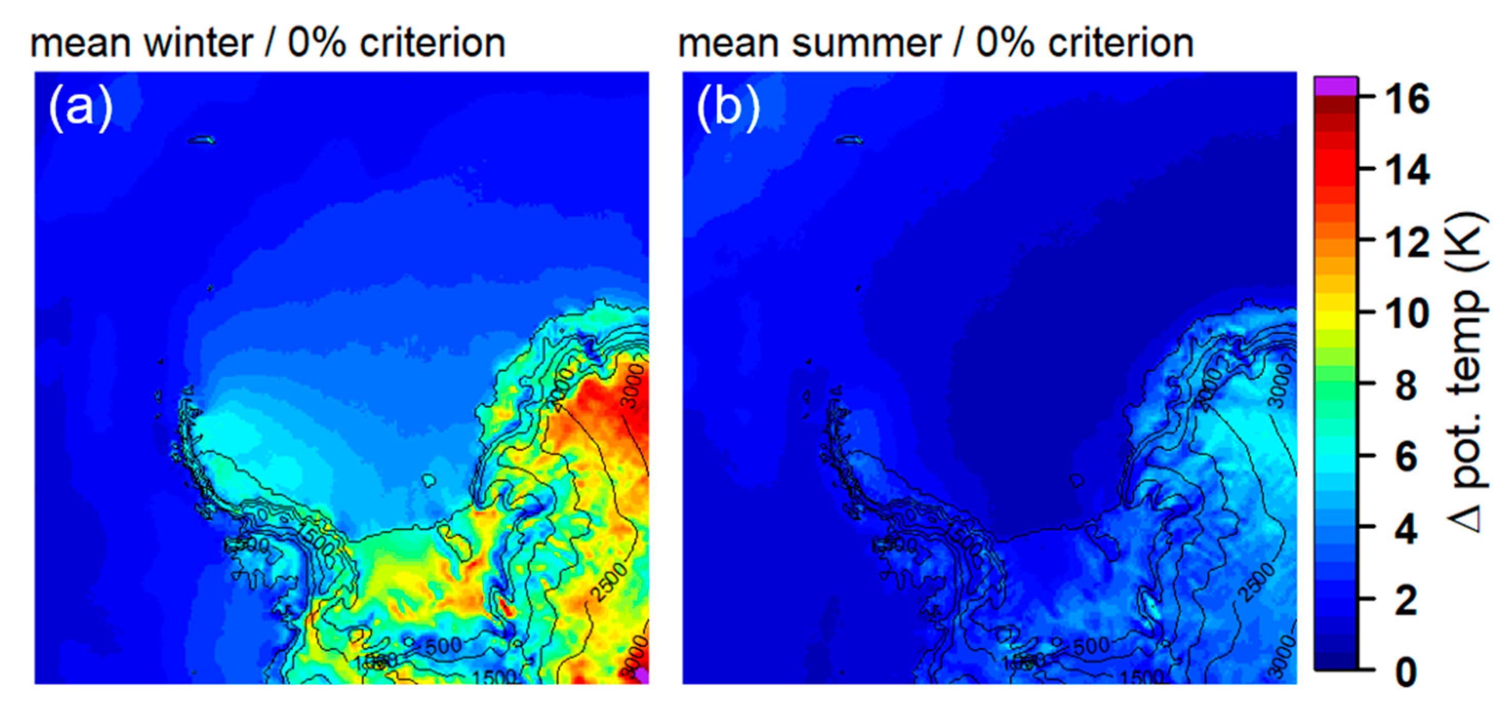
The height of the boundary layer is computed in CCLM as the height where the bulk Richardson number exceeds a value of 0.33 for the SBL [45] and 0.22 for the convective boundary layer (CBL) [46]. Additionally, we compute the height of the surface inversion or the height of an elevated inversion similar to [47]. In this method, the inversion height is computed as the height, where the gradient of the potential temperature drops from above to below a threshold value in a search from bottom to top. This is performed separately for surface inversions and elevated inversions (100 to 1000 m). Elevated inversions are typical for an SBL with strong winds such as katabatic or gap flows [34,47]. If no elevated inversion is found, surface inversions are searched by applying the same check starting at the surface.

This procedure is demonstrated by the LLJ case over the sea ice in Figure 3. This case during winter shows a well-mixed boundary layer for the lowest 200 m capped by an inversion. The maximum of the temperature gradient occurs at the inversion base, and the inversion height is determined as about 370 m, if a threshold of 2 K/100 m is taken. In this case study, the LLJ height is close to the inversion base, but below the inversion height. The LLJ shows a distinct directional shear of about 30° compared to the near-surface and mixed-layer values.

The used method determines the top of the inversion as the inversion height and is sensitive to the choice of the threshold for the temperature gradient. This choice follows other studies which used values of 2 K/100 m [47,48] or 1.5 K/100 m [9]. The sensitivity of the inversion height with respect to different thresholds is shown in Figure S1 in the supplement. A higher threshold leads to lower inversions over the inland ice and over the sea ice, but the sensitivity is relatively weak. A threshold of 2 K/100 m was taken for the evaluations of this study.

3. Results

3.1. Case Studies of LLJs

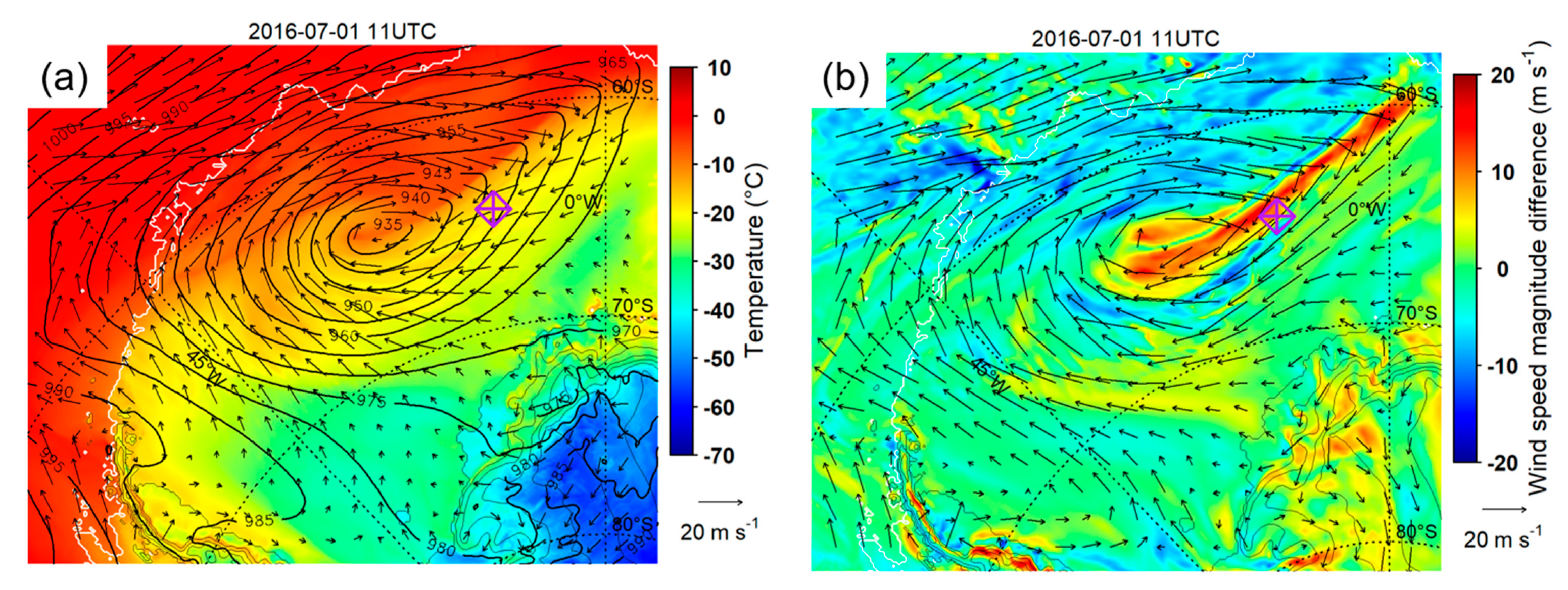
3.1.1. LLJ over the Sea Ice on 1 July 2016

The vertical profiles for this case were already shown in Figure 3. A very strong LLJ with 30 m/s is present at about 250 m. The decrease in the wind speed with height inside the search radius is 22%. When applying the relative criterion of 25%, as proposed by [44], this very strong LLJ would not be detected. The synoptic situation at 1100 UTC on 1 July 2016 is shown in Figure 5a. The profile shown in Figure 3 is located close to a frontal zone of a cyclone close to the sea ice edge. The 10 m wind is very high, south of the frontal zone. The wind speed difference between 200 m and 800 m shows a narrow zone of more than 10 m/s decrease of the wind with height (Figure 5b), which reflects that the LLJ extends over a large distance.

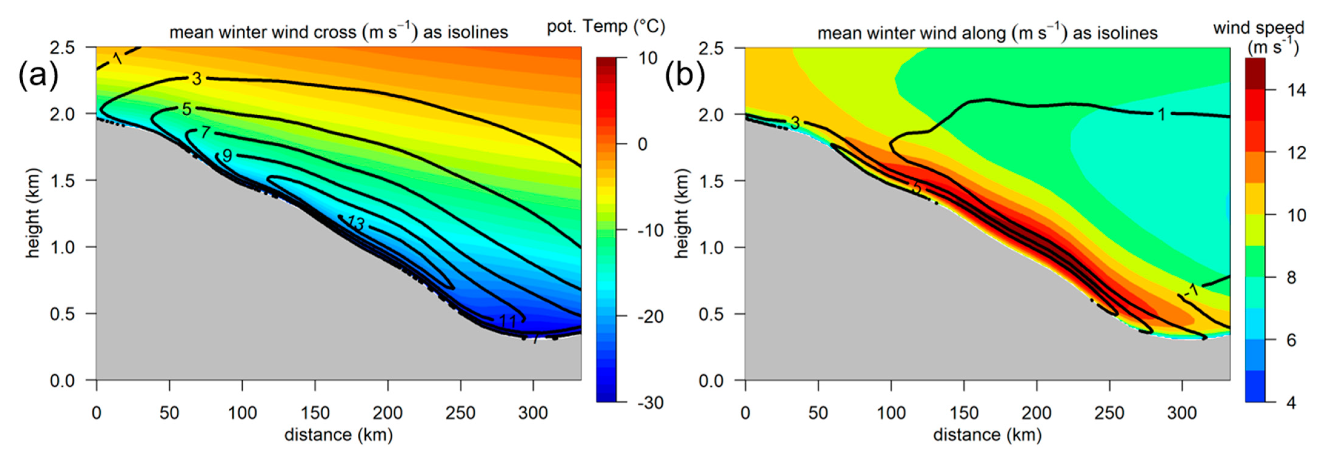
3.1.2. Katabatic LLJ over Coats Land on 10 June 2014

The vertical profiles for this case are shown in Figure 6 for 0500 UTC 10 June 2014, an overview of the synoptic situation is given in Figure 7. A well-defined LLJ with 17 m/s is present at about 50 m, which is at the height of the surface inversion. The wind minimum with less than 5 m/s is found at 400 m. Since the wind decrease with height inside the search radius is larger than 25%, this LLJ would have been also detected using the criteria of [44]. The wind direction turns slightly in the katabatic layer but shows a large change to southwesterly winds at a height of 400 m. Figure 7a shows that the katabatic wind over Coats Land is influenced by a cyclone with its center of the Brunt Ice Shelf (see Figure 1). The katabatic flow merges with the southwesterly flow along the coast associated with the cyclone (Figure 7b), which also dominates the flow above the katabatic layer. This is a case where the synoptic pressure gradient is opposite to the katabatic forcing. This situation was found also for other katabatic wind events over Coats Land by [24].

The main difference of this katabatic LLJ to the case of a baroclinic LLJ over the sea ice is that the wind speed in the lowest 50 m is much weaker in the katabatic layer, since the synoptic pressure gradient near the surface is very large for the baroclinic LLJ. In the katabatic case, the LLJ is associated with a surface inversion, while the baroclinic LLJ is at the top of a well-mixed boundary layer.

3.2. Wind Climatology of the ABL

Figure 8 shows the mean wind field at 10 m above the ground for the period 2002–2016. The different regimes of the near-surface wind can be clearly seen. Highest mean winds occur in the katabatic wind regime over the slopes of the ice sheet. The katabatic wind is also associated with the highest values of the directional constancy (directional constancy is defined as the ratio of the magnitude of the mean wind vector and the mean wind speed). The katabatic wind-field structure shows small-scale variations, which are a result of topographic channeling (Figure 1) but are also caused by the structures in the roughness length by subgrid-scale orography (Figure 2), since a high SSO SD leads to a large roughness length. As a second regime, the barrier flow at the east side of the Antarctic Peninsula can be seen as a flow parallel to the topography with increased values of the directional constancy. The northern part of the model domain is dominated by the westerly flow with increased wind, but relatively low constancy. Sea ice areas in the southern Weddell Sea as well as the area of the Filchner–Ronne Ice Shelf has weak wind and also low constancy. An exception is Berkner Island, which develops its own katabatic wind field with high constancy. The wind fields at 100, 200 and 500 m (supplementary material Figures S2–S4) show that the wind over the ice sheet has a downslope component at 100 m, but turns parallel to the topography isolines for 200 and 500 m.

More insight into the wind field structure can be obtained by cross-sections. Here, we focus on the wintertime situation for three regions (marked in Figure 1 and Figure 8 as A–C). For the katabatic wind region of Coats Land (Figure 9), the downslope wind component (along the cross-section) has values of more than 4 m/s only in a shallow layer above the surface (lowest 100 m). The across-slope wind component shows a low-level maximum of 9 m/s over the lower part of the slope. The potential temperature structure reflects the presence of an SBL over the slope. The mean wind speed shows an LLJ with a maximum of 12 m/s at about 200 m agl. This reflects that the katabatic wind is deflected to the left of the fall line by the Coriolis force (see Figure 8) and shows a vertical shear of the wind direction as the wind adjusts to the geostrophic balance with decreasing friction.

Cross-section A (Figure 10) represents the barrier wind region at the eastern side of the Antarctic Peninsula. The crosswind (north) component (Figure 10a) shows the barrier wind with a southerly wind maximum of more than 7 m/s below 500 m agl. The potential temperature reflects the strong static stability. The mean wind speed (Figure 10b) shows the barrier wind less well-defined with wind speeds of more than 11 m/s and a stronger maximum with more than 14 m/s near the top of the orography at the lee side of the mountains, which is associated with a strong westerly wind (along-wind component). Here, we see the impact of the flow over the mountain top generating downslope flow (as indicated also by the potential temperature structure over the upper part of the slope). It should be noted that the cross- and along-wind components are computed as means from all time steps, thus the magnitude of the mean wind vector is smaller than the mean wind speed.

Cross-section B (Figure 11) is located at the southern end of the FRIS. The wind field in the lowest 500 m is dominated by the crosswind component (Figure 11a), which shows a well-defined maximum at about 100 m agl. The mean wind speed is only slightly larger (Figure 11b). As for the katabatic wind of cross-section C the downslope wind component is much smaller (about 5 m/s) and is confined to a very shallow layer above the ground (Figure 11b). The field of the potential temperature structure shows the SBL over the slope.

3.3. Low-Level Jet Statistics

3.3.1. Comparison to Radiosonde Data

An extensive verification of CCLM simulations for the Antarctic with the same model data as used in the present study is shown by [31]. They conclude that the comparisons with the available radiosonde stations in the model area (see Figure 1) for 2002–2016 showed a wind speed bias close to 0 for the whole troposphere except for the lowest 2 km, where a slight positive bias of 2–3 m/s was found for stations near the Antarctic Peninsula (Marambio and Rothera), while the bias was smaller than 1 m/s for stations on ice shelves (Neumayer, Halley) and on the plateau (Amundsen-Scott).

The LLJ detection algorithm is applied to the radiosonde data from the five stations shown in Figure 1 and is compared to the results of the simulated profiles at the same position and time (Figure 12). Some problems were encountered concerning the radiosonde data availability, both in time and vertical levels (see

Table 1. Availability of radiosonde data for 2002–2016 (see Figure 1).

Station	Profiles	Data Gaps	Remarks
Marambio	1364	2007–2008	Sparse data in 2002–2009
Neumayer	5355	no
Rothera	1021	2008–2011	No data for 8 to 11 months per year in 2002–2012
Halley	4877	no
Amundsen-Scott	7664	no	Vertical resolution in the lowest 500 m for 2002–2004 is too coarse to detect LLJs

).

Overall, there is good agreement except for the Amundsen-Scott station at the south pole. Here the number of LLJs with heights at about 100 m is much larger in the simulations than in the radiosonde data. Since only few LLJs have heights larger than 200 m, this has an impact on all distributions at that station. It is known that the wind profile from radiosondes is inaccurate for low levels, since the balloon has to adapt to the ambient wind speed, the wind field is disturbed by obstacles and buildings, and errors occur by the pendulum motion of the radiosonde, which is corrected by a low-pass filter, which results in a vertical resolution of 200 m [49]. The distributions of LLJ heights and speeds are almost identical for Neumayer and Halley, broader distributions are found in the simulations for Marambio and Rothera. The distributions of the relative wind speed change within the search radius show the problem of the choice of the relative criterion. Since the maxima lie between 0.1 and 0.3 (10–30%) for most stations, the application of a relative criterion of 25% as proposed by [44] will miss a large part of LLJs. This indicates that a value of 25% for this criterion seems to be too restrictive, particularly at very high wind speeds. The overall statistics for all LLJs detected in the CCLM and RS data sets are shown in

Table 2. Statistics of LLJs from radiosonde (RS) and model data for 2002–2016 for all LLJs (mean values are given for CCLM data, bias is CCLM-RS).

Station	Frequency in %		Height in m		Speed in m/s		Rel. Speed Change in %
	RS	CCLM	Mean	Bias	Mean	Bias	Mean	Bias
Marambio	32	33	315	−17	14.0	1.3	30	−4
Neumayer	48	41	286	−84	17.0	−1.1	27	0
Rothera	30	37	531	53	18.0	6.9	30	−12
Halley	46	39	291	−50	14.3	0.9	30	−5
Amundsen-Scott	14	55	102	−150	12.9	−0.3	33	7

. The bias for the jet height has reasonable values, if the height exceeds 200 m. The bias in speed is small except for Rothera, where the local topography influences on the wind field might not be adequately represented in the simulations with 15 km resolution.

All LLJs occur in SBL conditions for all stations. The potential temperature difference between at the jet height and the surface for the simulated and observed LLJs is similar for all stations except at the south pole. The change of the wind direction between the jet height and 5 m is mostly negative, although for Marambio and Rothera some LLJs have a positive change in wind direction. The bias towards negative values reflects that the change of the wind direction with height is consistent with the decreasing friction with height.

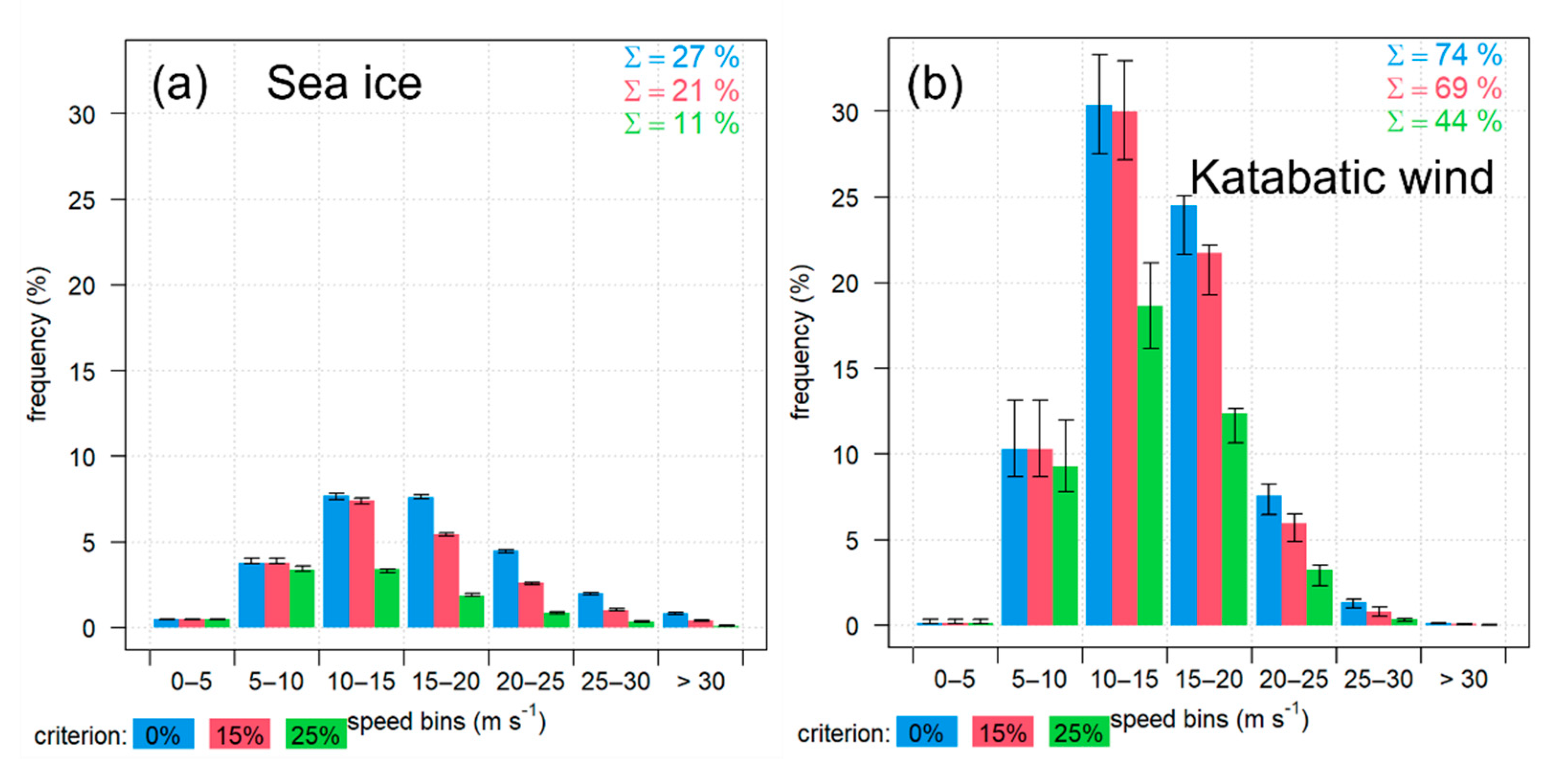
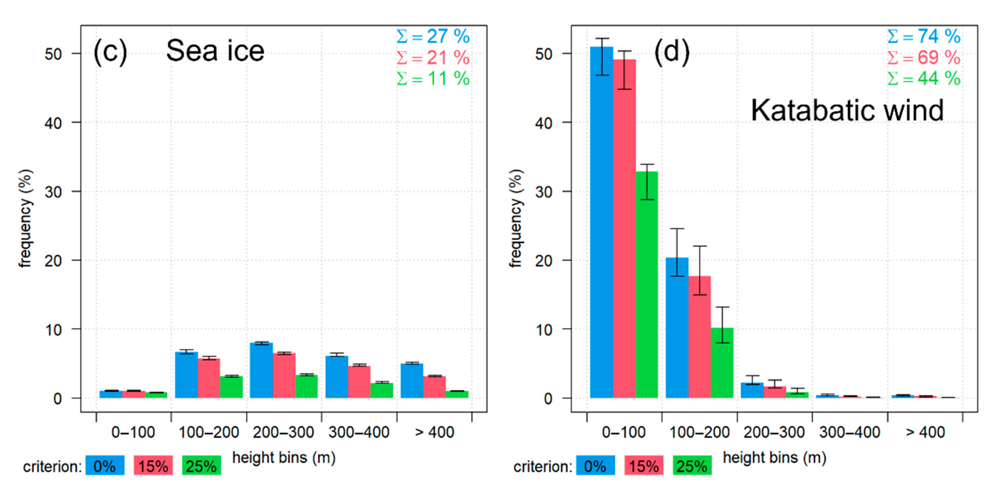
3.3.2. Climatology from Model Simulations

Figure 13 shows the LLJ frequency for 2002–2016 for the winter (April–September), the summer (December–January) and the annual average. The annual average is clearly dominated by the winter period. All months except December and January were found to show similar LLJ frequencies. In summer (December–January), the katabatic wind shows a clear daily cycle and is much weaker compared to winter months. This reduces the LLJ frequency over the ice sheet from more than 80% in winter to less than 40% in summer.

The winter average of the LLJ speed for 2002–2016 is shown in Figure 14a. This distribution has to be interpreted together with the frequency distribution (Figure 13a). The mean LLJ speed in the katabatic wind regime is about 15 m/s, but 20 m/s is also exceeded in some areas. The barrier wind regime, which has medium values of LLJ frequency, shows values of 15–20 m/s. The mean LLJ speed increases towards the northern Weddell Sea, but the LLJ frequency is below 30% in these areas. The inter monthly standard deviation of the LLJ speed (not shown) has a very high variability in regions with high sub-grid variance of the orography and in the coastal zone of the eastern Weddell Sea, where the wind field is dominated by cyclones moving from the northern Weddell Sea towards the Antarctic coast. The winter average of the LLJ height (Figure 14b) is generally below 150 m for the inland ice, and around 200–300 m over the sea ice. Plots for the summer and annual average (supplementary material Figure S8) show that the LLJs over the ice sheet are much weaker during summer.

More insight into the statistics of LLJ characteristics can be obtained by looking at the distribution functions of hourly values of LLJ height and speed. Figure 15 shows these distributions for selected grid points over ocean/sea ice (point 1 in Figure 1) and inland ice (point 6 in Figure 1) for three different values of the relative criterium (0, 15 and 25%). Over the ocean area, the LLJ heights are distributed almost equally over all height ranges (Figure 15c). The speed distribution shows a very broad maximum and a large dependency on the choice of the relative criterion (Figure 15a). For the katabatic wind regime, almost all LLJs are below 200 m (Figure 15d), while the speed distribution shows a clear maximum for 10–20 m/s and an asymmetric shape (Figure 15b). The choice of 0% or 15% for the relative criterion has only a small influence, but a value of 25% reduces the number of LLJs considerably. A plot summarizing the statistics for different subareas is shown in Figures S9 and S10 in the Supplementary Materials.

As further LLJ characteristics, we look at the duration of the LLJs. The statistics of the LLJ event durations is shown in Figure 16 for the selected points shown in Figure 1. A LLJ event is defined as the period where in consecutive profiles the LLJ criteria are fulfilled and the height of the LLJ shows no large jumps. As expected from the results presented above, there are more and longer LLJs in winter than in summer. These differences are small over the ocean/sea ice (OC), where there is only a slight increase in LLJs lasting more than one day. The same holds for LLJs over the FRIS (FR). The seasonal differences are most pronounced over the ice sheet (IS), where LLJs with a duration of more than 1 day occur frequently during winter. The barrier wind region at the Antarctic Peninsula (A) shows also an increase in the LLJ duration during winter, particularly for events with more than 24 h duration. At Coats Land (C), LLJs with less than 1 day duration dominate during winter and summer. For cross-section B in the southern part of the FRIS, the high frequencies of LLJs are found in both seasons, and the fraction of LLJs with longer duration increases in winter. It has to be noted that the statistics of LLJ durations is sensitive to the relative criterion (see Figure S18 in the Supplementary Materials). When increasing the relative criterion, the length of LLJ events decreases and less LLJs lasting longer than 10 days are found over the ice sheet.

The seasonal differences of the duration of events seem to be related to the daily cycle during summer, but also to generally weaker winds during summer compared to winter. For higher winds, it is more likely that the absolute LLJ criterion is exceeded more frequently and that the duration is longer. If the LLJ wind anomaly is less than 2 m/s for some period during the LLJ development, a long LLJ will be split into separate shorter events. The seasonality of the LLJ strength is most pronounced over the ice sheet, while it is relatively weak over the sea ice and ocean areas (see Figure 14 and Figure S8). The duration of katabatic LLJs near the coast in the eastern Weddell Sea (cross-section C) is also influenced by the transient cyclones passing over the Weddell Sea or by mesocyclones developing near the coast [50].

The directional shear between the jet and the lowest model level (5 m) is negative in the average for all regions and seasons (not shown). This reflects that the change of the wind direction with height is consistent with the decreasing friction with height. The LLJ stability (difference between the potential temperature at the jet height and the surface) is shown in Figure 17 (boundary layer height and inversion statistics are presented in the Supplementary Materials, Figures S11–S17). While during winter the inversion frequency is higher than 90% over the inland ice, the FRIS and the sea ice (Figure S12), the inversion strength exceeds 15K only over the inland ice and the FRIS (Figure S14). This pattern is similar for the LLJ stability (Figure 17), and low values of stability correspond to high LLJ speeds (Figure 14), which reflects the strong mixing associated with the jets. This mixing seems to strongly affect the strength of the surface inversion (Figure S17). LLJs during summer are associated with relative weak surface inversions and LLJ stability (Figure 17 and Figure S17).

4. Discussion

This study presents the first RCM-based climatology of LLJs for the Antarctic. It uses a similar approach as the model-based study of [44], who used reanalysis data with 30 km resolution for 11 years for the Arctic. Some findings of [44] are qualitatively similar to our results: highest frequencies of LLJs in katabatic wind regions (Greenland) and low frequency of LLJs over the sea ice of the central Arctic. Other findings associated with, e.g., tip jets at Greenland and topographic effects over Siberia cannot be compared to the Antarctic conditions.

The results of the present study have shown that the SSO parameterization has a distinct effect on the wind field and LLJ statistics over the inland ice. The SSO scheme was introduced in CCLM in order to describe the momentum drag in mountain areas more realistically [41]. Ref. [51] propose a modification of the SSO scheme for the SBL by applying the scheme only for model grid cells where the boundary layer height is two times larger than the SSO standard deviation. Although the SBL height in the katabatic wind is typically smaller than 300 m (see Figure S11 in the Supplementary Materials), this modification would reduce the SSO effects over the ice sheet only for a few grid points, since the SSO standard deviation is generally smaller than 40 m. While the first published simulations of the near-surface wind over the ice sheet showed a very smooth wind field structure [52], recent simulations show a more detailed structure due to the consideration of topographic grid-scale and sub-grid scale (e.g., [30]).

Cross-sections for katabatic wind regions show similar structures as found by [30]. Due to the horizontal temperature gradient caused by the sloped inversion in the katabatic SBL, downslope winds are found only close to the surface and the wind turns to directions perpendicular to the slope within a few hundred meters. Barrier winds at the Antarctic Peninsula were mainly described for the near-surface wind in previous studies [16,24,53], in our study we can show that they are associated with a clear wind maximum at about 300 m in the winter climatology, and that they are associated with strong LLJs for more than half the time during the winter months.

The sensitivity of the results to the criteria to identify LLJs is an important issue for SBL studies in polar regions. While the absolute criterion of 2 m/s for the LLJ wind anomaly is generally used [5,6,54,55], the relative criterion of the wind speed decrease above the wind maximum introduced by [54] and used in [44] can affect the results of an LLJ climatology. We find that the value of 25% of the relative criterion used in [44,54] is too restrictive, and we propose to use only the absolute criterion for model studies. The sensitivity of the results to this criterion is different for different regions. It has larger effects for the LLJ frequency over sea ice than for the katabatic LLJs. In contrast, the length of katabatic LLJ events shows a large sensitivity with respect to the relative criterion. If the LLJ wind anomaly gets less pronounced for some period during the LLJ development, a long LLJ will be split into two separate shorter events. This effect may explain a large part of the sensitivity.

In order to simulate SBL features as LLJs and surface inversions, adequate horizontal and vertical resolutions are necessary. Very shallow LLJs with heights below 35 m as observed at Dome C by [14] are hardly simulated with the vertical resolution used in our study, where the lowest model levels are at 5, 16 and 27 m. However, most of the LLJs shown by [14] were weak and would likely not pass the absolute criterion of LLJs. For typical katabatic winds over the ice sheet, the used vertical resolution with 10 levels below 300 m is sufficient to resolve katabatic LLJs. The horizontal resolution is important in areas with small-scale structures of the topography such as the Antarctic Peninsula. A long-term comparison (2002–2016) of CCLM simulations with 15 and 5 km resolution by [31] for the Weddell Sea region shows only small differences between these resolutions for the ice sheet and the ocean/sea ice areas. A comparison between CCLM simulations at different resolutions (15, 5 and 2 km) as well as ERA-Interim and ERA5 re-analyses (80 km and 30 km horizontal resolution, respectively) is shown in Figure 18 for the area of the Larsen Ice Shelf for July 2016 for the 10 m-wind. The re-analyses are not able to account for the topographic effects of katabatic winds and foehn in that region. With 15 km resolution, these effects are simulated but underestimated. This is in accordance with the findings of [56,57], who concluded that foehn effects over Larsen-C Ice Shelf are best represented for a model with 1.5 km resolution. However, simulations with a kilometer scale resolution are not feasible for larger domains over a long period.

The LLJ characteristics show only little interannual variation (see Figure S19 in the Supplementary Materials). As a future research direction, the methodology of this paper is planned to be applied to the investigation of LLJ characteristics during climate change. CCLM simulations for climate change scenarios for the whole Antarctic are currently performed and evaluated.

References

1. Gorodetskaya, I.V.; Tsukernik, M.; Claes, K.; Ralph, M.F.; Neff, W.D.; van Lipzig, N.P.M. The role of atmospheric rivers in anomalous snow accumulation in East Antarctica. Geophys. Res. Lett. 2014, 41, 6199–6206. [Google Scholar] [CrossRef] [Green Version]
2. Zentek, R.; Kohnemann, S.H.E.; Heinemann, G. Analysis of the performance of a ship-borne scanning wind lidar in the Arctic and Antarctic. Atmos. Meas. Tech. 2018, 11, 5781–5795. [Google Scholar] [CrossRef] [Green Version]
3. Guest, P.; Persson, P.O.G.; Wang, S.; Jordan, M.; Jin, Y.; Blomquist, B.; Fairall, C. Low-Level Baroclinic Jets Over the New Arctic Ocean. J. Geophys. Res. Oceans 2018, 123, 4074–4091. [Google Scholar] [CrossRef]
4. Jakobson, L.; Vihma, T.; Jakobson, E.; Palo, T.; Männik, A.; Jaagus, J. Low-level jet characteristics over the Arctic Ocean in spring and summer. Atmos. Chem. Phys. 2013, 13, 11089–11099. [Google Scholar] [CrossRef] [Green Version]
5. Heinemann, G.; Drüe, C.; Schwarz, P.; Makshtas, A. Observations of Wintertime Low-Level Jets in the Coastal Region of the Laptev Sea in the Siberian Arctic Using SODAR/RASS. Remote Sens. 2021, 13, 1421. [Google Scholar] [CrossRef]
6. Andreas, E.L.; Claffy, K.J.; Makshtas, A.P. Low-Level Atmospheric Jets and Inversions over the Western Weddell Sea. Bound.-Layer Meteorol. 2000, 97, 459–486. [Google Scholar] [CrossRef]
7. Heinemann, G.; Rose, L. Surface energy balance, parameterizations of boundary-layer heights and the application of resistance laws near an Antarctic Ice Shelf front. Bound.-Layer Meteorol. 1990, 51, 123–158. [Google Scholar] [CrossRef]
8. Heinemann, G. Aircraft-Based Measurements Of Turbulence Structures In The Katabatic Flow Over Greenland. Bound.-Layer Meteorol. 2002, 103, 49–81. [Google Scholar] [CrossRef]
9. Heinemann, G. The KABEG’97 field experiment: An aircraft-based study of katabatic wind dynamics over the Greenland ice sheet. Bound.-Layer Meteorol. 1999, 93, 75–116. [Google Scholar] [CrossRef]
10. Renfrew, I.A.; Anderson, P.S. Profiles of katabatic flow in summer and winter over Coats Land, Antarctica. Q. J. R. Meteorol. Soc. 2006, 132, 779–802. [Google Scholar] [CrossRef] [Green Version]
11. Wendler, G. Strong gravity flow observed along the slope of Eastern Antarctica. Meteorl. Atmos. Phys. 1990, 43, 127–135. [Google Scholar] [CrossRef]
12. Loewe, F. The land of storms. Weather 1972, 27, 110–121. [Google Scholar] [CrossRef]
13. Kodama, Y.; Wendler, G.; Ishikawa, N. The Diurnal Variation of the Boundary Layer in Summer in Adelie Land, Eastern Antarctica. J. Appl. Meteor. 1989, 28, 16–24. [Google Scholar] [CrossRef] [Green Version]
14. Gallée, H.; Barral, H.; Vignon, E.; Genthon, C. A case study of a low-level jet during OPALE. Atmos. Chem. Phys. 2015, 15, 6237–6246. [Google Scholar] [CrossRef] [Green Version]
15. Vignon, É.; Traullé, O.; Berne, A. On the fine vertical structure of the low troposphere over the coastal margins of East Antarctica. Atmos. Chem. Phys. 2019, 19, 4659–4683. [Google Scholar] [CrossRef] [Green Version]
16. Schwerdtfeger, W. Meteorological aspects of the drift of ice from the Weddell Sea toward the mid-latitude westerlies. J. Geophys. Res. 1979, 84, 6321. [Google Scholar] [CrossRef]
17. Nigro, M.A.; Cassano, J.J.; Lazzara, M.A.; Keller, L.M. Case Study of a Barrier Wind Corner Jet off the Coast of the Prince Olav Mountains, Antarctica. Mon. Weather Rev. 2012, 140, 2044–2063. [Google Scholar] [CrossRef]
18. O’Connor, W.P.; Bromwich, D.H.; Carrasco, J.F. Cyclonically Forced Barrier Winds along the Transantarctic Mountains near Ross Island. Mon. Weather Rev. 1994, 122, 137–150. [Google Scholar] [CrossRef] [Green Version]
19. Elvidge, A.D.; Renfrew, I.A.; King, J.C.; Orr, A.; Lachlan-Cope, T.A.; Weeks, M.; Gray, S.L. Foehn jets over the Larsen C Ice Shelf, Antarctica. Q. J. R. Meteorol. Soc. 2015, 141, 698–713. [Google Scholar] [CrossRef] [Green Version]
20. Orr, A.; Kirchgaessner, A.; King, J.; Phillips, T.; Gilbert, E.; Elvidge, A.; Weeks, M.; Gadian, A.; Kuipers Munneke, P.; Broeke, M.; et al. Comparison of kilometre and sub-kilometre scale simulations of a foehn wind event over the Larsen C Ice Shelf, Antarctic Peninsula using the Met Office Unified Model (MetUM). Q. J. R. Meteorol. Soc. 2021, 147, 3472–3492. [Google Scholar] [CrossRef]
21. KING, J.C.; Lachlan-Cope, T.A.; Ladkin, R.S.; Weiss, A. Airborne Measurements in the Stable Boundary Layer over the Larsen Ice Shelf, Antarctica. Bound.-Layer Meteorol. 2008, 127, 413–428. [Google Scholar] [CrossRef] [Green Version]
22. Seefeldt, M.W.; Cassano, J.J. An Analysis of Low-Level Jets in the Greater Ross Ice Shelf Region Based on Numerical Simulations. Mon. Weather Rev. 2008, 136, 4188–4205. [Google Scholar] [CrossRef]
23. Parish, T.R.; Bromwich, D.H. Reexamination of the Near-Surface Airflow over the Antarctic Continent and Implications on Atmospheric Circulations at High Southern Latitudes. Mon. Weather Rev. 2007, 135, 1961–1973. [Google Scholar] [CrossRef]
24. Ebner, L.; Heinemann, G.; Haid, V.; Timmermann, R. Katabatic winds and polynya dynamics at Coats Land, Antarctica. Antarct. Sci. 2014, 26, 309–326. [Google Scholar] [CrossRef]
25. Tastula, E.-M.; Vihma, T.; Andreas, E.L. Evaluation of Polar WRF from Modeling the Atmospheric Boundary Layer over Antarctic Sea Ice in Autumn and Winter. Mon. Weather Rev. 2012, 140, 3919–3935. [Google Scholar] [CrossRef]
26. Van Lipzig, N.P.M.; Turner, J.; Colwell, S.R.; van den Broeke, M.R. The near-surface wind field over the Antarctic continent. Int. J. Climatol. 2004, 24, 1973–1982. [Google Scholar] [CrossRef] [Green Version]
27. Souverijns, N.; Gossart, A.; Demuzere, M.; Lenaerts, J.T.M.; Medley, B.; Gorodetskaya, I.V.; Vanden Broucke, S.; van Lipzig, N.P.M. A New Regional Climate Model for POLAR-CORDEX: Evaluation of a 30-Year Hindcast with COSMO-CLM 2 over Antarctica. J. Geophys. Res. 2019, 124, 1405–1427. [Google Scholar] [CrossRef] [Green Version]
28. Van Wessem, J.M.; van de Berg, W.J.; Noël, B.P.Y.; van Meijgaard, E.; Amory, C.; Birnbaum, G.; Jakobs, C.L.; Krüger, K.; Lenaerts, J.T.M.; Lhermitte, S.; et al. Modelling the climate and surface mass balance of polar ice sheets using RACMO2—Part 2: Antarctica (1979–2016). Cryosphere 2018, 12, 1479–1498. [Google Scholar] [CrossRef] [Green Version]
29. Lenaerts, J.T.M.; Vizcaino, M.; Fyke, J.; van Kampenhout, L.; van den Broeke, M.R. Present-day and future Antarctic ice sheet climate and surface mass balance in the Community Earth System Model. Clim. Dyn. 2016, 47, 1367–1381. [Google Scholar] [CrossRef] [Green Version]
30. Van de Berg, W.J.; van den Broeke, M.R.; van Meijgaard, E. Heat budget of the East Antarctic lower atmosphere derived from a regional atmospheric climate model. J. Geophys. Res. 2007, 112. [Google Scholar] [CrossRef] [Green Version]
31. Zentek, R.; Heinemann, G. Verification of the regional atmospheric model CCLM v5.0 with conventional data and lidar measurements in Antarctica. Geosci. Model Dev. 2020, 13, 1809–1825. [Google Scholar] [CrossRef] [Green Version]
32. Kohnemann, S.H.E.; Heinemann, G.; Bromwich, D.H.; Gutjahr, O. Extreme Warming in the Kara Sea and Barents Sea during the Winter Period 2000–16. J. Clim. 2017, 30, 8913–8927. [Google Scholar] [CrossRef]
33. Kohnemann, S.H.; Heinemann, G. A climatology of wintertime low-level jets in Nares Strait. POLAR 2021, 40. [Google Scholar] [CrossRef]
34. Heinemann, G. Assessment of Regional Climate Model Simulations of the Katabatic Boundary Layer Structure over Greenland. Atmosphere 2020, 11, 571. [Google Scholar] [CrossRef]
35. Gutjahr, O.; Heinemann, G.; Preußer, A.; Willmes, S.; Drüe, C. Quantification of ice production in Laptev Sea polynyas and its sensitivity to thin-ice parameterizations in a regional climate model. Cryosphere 2016, 10, 2999–3019. [Google Scholar] [CrossRef] [Green Version]
36. Dee, D.P.; Uppala, S.M.; Simmons, A.J.; Berrisford, P.; Poli, P.; Kobayashi, S.; Andrae, U.; Balmaseda, M.A.; Balsamo, G.; Bauer, P.; et al. The ERA-Interim reanalysis: Configuration and performance of the data assimilation system. Q. J. R. Meteorol. Soc. 2011, 137, 553–597. [Google Scholar] [CrossRef]
37. Schröder, D.; Heinemann, G.; Willmes, S. The impact of a thermodynamic sea-ice module in the COSMO numerical weather prediction model on simulations for the Laptev Sea, Siberian Arctic. Polar Res. 2011, 30, 6334. [Google Scholar] [CrossRef]
38. Spreen, G.; Kaleschke, L.; Heygster, G. Sea ice remote sensing using AMSR-E 89-GHz channels. J. Geophys. Res. 2008, 113, 14485. [Google Scholar] [CrossRef] [Green Version]
39. Kurtz, N.T.; Markus, T. Satellite observations of Antarctic sea ice thickness and volume. J. Geophys. Res. 2012, 117. [Google Scholar] [CrossRef] [Green Version]
40. Schaffer, J.; Timmermann, R.; Arndt, J.E.; Kristensen, S.S.; Mayer, C.; Morlighem, M.; Steinhage, D. A global, high-resolution data set of ice sheet topography, cavity geometry, and ocean bathymetry. Earth Syst. Sci. Data 2016, 8, 543–557. [Google Scholar] [CrossRef] [Green Version]
41. Doms, G.; Förstner, J.; Heise, H.; Herzog, H.-J.; Mironov, D.; Raschendorfer, M.; Reinhardt, T.; Ritter, B.; Schrodin, R.; Schulz, J.-P.; et al. A Description of the Nonhydrostatic Regional COSMO-Model. Part II. Physical Parameterizations; Deutscher Wetterdienst: Offenbach, Germany, 2013. [Google Scholar]
42. Lott, F.; Miller, M.J. A new subgrid-scale orographic drag parametrization: Its formulation and testing. Q. J. R. Meteorol. Soc. 1997, 123, 101–127. [Google Scholar] [CrossRef]
43. Zentek, R. COSMO Documentation (Archived Version from 2019, Uploaded with Permission of the DWD). 2019. Available online: https://zenodo.org/record/3339384 (accessed on 7 May 2021).
44. Tuononen, M.; Sinclair, V.A.; Vihma, T. A climatology of low-level jets in the mid-latitudes and polar regions of the Northern Hemisphere. Atmos. Sci. Lett. 2015, 16, 492–499. [Google Scholar] [CrossRef] [Green Version]
45. Wetzel, P.J. Toward Parameterization of the Stable Boundary Layer. J. Appl. Meteor. 1982, 21, 7–13. [Google Scholar] [CrossRef]
46. Vogelezang, D.H.P.; Holtslag, A.A.M. Evaluation and model impacts of alternative boundary-layer height formulations. Bound.-Layer Meteorol. 1996, 81, 245–269. [Google Scholar] [CrossRef]
47. Heinemann, G. An Aircraft-Based Study of Strong Gap Flows in Nares Strait, Greenland. Mon. Weather Rev. 2018, 146, 3589–3604. [Google Scholar] [CrossRef]
48. Heinemann, G.; Klein, T. Modelling and observations of the katabatic flow dynamics over Greenland. Tellus A 2002, 54, 542–554. [Google Scholar] [CrossRef]
49. Dirksen, R.J.; Sommer, M.; Immler, F.J.; Hurst, D.F.; Kivi, R.; Vömel, H. Reference quality upper-air measurements: GRUAN data processing for the Vaisala RS92 radiosonde. Atmos. Meas. Tech. 2014, 7, 4463–4490. [Google Scholar] [CrossRef] [Green Version]
50. Heinemann, G. Mesoscale Vortices in the Weddell Sea Region (Antarctica). Mon. Weather Rev. 1990, 118, 779–793. [Google Scholar] [CrossRef] [Green Version]
51. Tsiringakis, A.; Steeneveld, G.J.; Holtslag, A.A.M. Small-scale orographic gravity wave drag in stable boundary layers and its impact on synoptic systems and near-surface meteorology. Q. J. R. Meteorol. Soc. 2017, 143, 1504–1516. [Google Scholar] [CrossRef]
52. Parish, T.R.; Bromwich, D.H. Continental-Scale Simulation of the Antarctic Katabatic Wind Regime. J. Clim. 1991, 4, 135–146. [Google Scholar] [CrossRef] [Green Version]
53. Van Wessem, J.M.; Reijmer, C.H.; van de Berg, W.J.; van den Broeke, M.R.; Cook, A.J.; van Ulft, L.H.; van Meijgaard, E. Temperature and Wind Climate of the Antarctic Peninsula as Simulated by a High-Resolution Regional Atmospheric Climate Model. J. Clim. 2015, 28, 7306–7326. [Google Scholar] [CrossRef] [Green Version]
54. Baas, P.; Bosveld, F.C.; Klein Baltink, H.; Holtslag, A.A.M. A Climatology of Nocturnal Low-Level Jets at Cabauw. J. Appl. Meteor. Climatol. 2009, 48, 1627–1642. [Google Scholar] [CrossRef]
55. Karipot, A.; Leclerc, M.Y.; Zhang, G. Characteristics of Nocturnal Low-Level Jets Observed in the North Florida Area. Mon. Weather Rev. 2009, 137, 2605–2621. [Google Scholar] [CrossRef]
56. Elvidge, A.D.; Renfrew, I.A.; King, J.C.; Orr, A.; Lachlan-Cope, T.A. Foehn warming distributions in nonlinear and linear flow regimes: A focus on the Antarctic Peninsula. Q. J. R. Meteorol. Soc. 2016, 142, 618–631. [Google Scholar] [CrossRef] [Green Version]
57. Turton, J.V.; Kirchgaessner, A.; Ross, A.N.; King, J.C. Does high-resolution modelling improve the spatial analysis of föhn flow over the Larsen C Ice Shelf? Weather 2017, 72, 192–196. [Google Scholar] [CrossRef] [Green Version]
Figure 1. Model domain of CCLM with topography (shaded and isolines every 500 m) and sea ice area (white) for a day in winter (iceberg A23A marked). The dashed box shows the area used for the evaluation, A, B and C mark cross-sections. The red squares mark specific areas for case studies and statistics. FRIS = Filchner-Ronne Ice Shelf, LCIS = Larsen-C Ice Shelf, BIS = Brunt Ice Shelf. Black triangles mark radiosonde stations inside the evaluation domain.
Atmosphere 12 01635 g001
Figure 2. (a) Standard deviation of the sub-grid scale orography (SSO). (b) Roughness length over the land areas. The dashed box shows the area used for the evaluation.
Atmosphere 12 01635 g002
Figure 3. Overview of the vertical search algorithm for the inversion height (hinv), inversion strength (Δθinv), LLJ height (hjet), LLJ speed (vjet), LLJ temperature difference (Δθjet), and LLJ wind direction difference (Δϕjet). Vertical profiles are shown for potential temperature (red), gradient of potential temperature (orange), wind speed (blue), gradient of wind speed (purple) and wind direction (green) for a grid point over sea ice (point 1 in Figure 1) at 1100 UTC on 1 July 2016. The light blue bar shows the search radius, the relative decrease within the search radius is given in percent. Dots mark the model levels.
Atmosphere 12 01635 g003
Figure 4. LLJ frequency for 2002–2016 for different relative criteria (all with 2 m/s absolute criterion).
Atmosphere 12 01635 g004
Figure 5. (a) Mean sea level pressure (MSLP, isolines every 5 hPa), 2 m temperature (color bar) and 10 m-wind vector (at every 10th grid point) and (b) wind speed difference between 200 m and 800 m and 200 m-wind vectors for 1100 UTC 1 July 2016 for a subregion of the model domain. The diamond marks the location of the wind profile of Figure 3. The sea ice edge is marked by a thick white line. Topography is shown as grey isolines every 500 m.
Atmosphere 12 01635 g005
Figure 6. Vertical profiles of the potential temperature (red), wind speed (blue), and wind direction (green) for a grid point over Coats Land (point 2 in Figure 1) for 0500 UTC 10 June 2014 (see Figure 7 for the location). The light blue bar shows the search radius, the relative decrease within the search radius is given in percent. Dots mark the model levels.
Atmosphere 12 01635 g006
Figure 7. (a) Mean sea level pressure (MSLP, isolines every 5 hPa), 2 m temperature (color bar) and 10 m-wind vector (at every 10th grid point) for the Weddell Sea region and (b) 10 m-wind speed (color bar) and 10 m-wind vector (at every 2nd grid point) for 0500 UTC 10 June 2014 for a subregion of the model domain (marked by the box in (a)). The diamond marks the location of the wind profile of Figure 6. Topography is shown as gray and black isolines every 500 m in (a) and (b), respectively.
Atmosphere 12 01635 g007
Figure 8. Mean wind field for 2002–2016 at 10 m. (a) Mean wind vector (at every 10th grid point) and wind speed, (b) directional constancy with streamlines. Topography is shown as black and white isolines every 500 m in (a) and (b), respectively. Cross-sections A, B and C are marked (see also Figure 1).
Atmosphere 12 01635 g008
Figure 9. Cross-section C in the katabatic wind region over Coats Land (see Figure 1 and Figure 8) for April–September 2002–2016 for (a) the crosswind component (isolines every 1 m/s) and the potential temperature (color scale) and (b) the along-wind (downslope) component (isolines every 1 m/s) and the mean wind speed (color scale).
Atmosphere 12 01635 g009
Figure 10. Cross-section A in the barrier wind region at the Antarctic Peninsula (see Figure 1 and Figure 8) for April–September 2002–2016 for (a) the crosswind (north) component (isolines every 1 m/s) and the potential temperature (color scale) and (b) the along-wind (east) component (isolines every 1 m/s) and the mean wind speed (color scale).
Atmosphere 12 01635 g010
Figure 11. Cross-section B in the southern part of the FRIS (see Figure 1 and Figure 8) for April–September 2002–2016 for (a) the crosswind component (isolines every 2 m/s) and the potential temperature (color scale) and (b) the along-wind (downslope) component (isolines every 2 m/s) and the mean wind speed (color scale).
Atmosphere 12 01635 g011
Figure 12. Distribution functions (absolute frequencies, total frequencies in the first column) of LLJ characteristics from radiosondes (black) and CCLM simulations (blue) for 2002–2016. The different radiosonde stations are in the rows, the columns show distribution functions of LLJ height (in m), LLJ speed (in m/s), the relative wind speed change within the search radius, the potential temperature difference between the jet height and the surface (in K), and the change of the wind direction (in °) between the jet height and 5 m. Note the unequal bin width of LLJ height and potential temperature difference.
Atmosphere 12 01635 g012
Figure 13. LLJ frequency for 2002–2016 for the winter (a), the summer (b,c) the annual average.
Atmosphere 12 01635 g013
Figure 14. Winter (April–September) average of the (a) LLJ speed and (b) LLJ height for 2002–2016.
Atmosphere 12 01635 g014
Figure 15. Distribution functions (absolute frequencies, total frequencies in the respective colors) of LLJ height and speed based on hourly values using different relative criteria (color bars) for winters 2002–2016 for location 1 (sea ice, (a,c)) and location 6 (inland ice, (b,d), see Figure 1 for positions). The whiskers indicate the maximum and minimum values for the surrounding 24 grid points. The overall frequencies for the different relative criteria a shown as numbers in the respective colors.
Atmosphere 12 01635 g015aAtmosphere 12 01635 g015b
Figure 16. Distribution for the length of LLJ events (fraction of time of the respective LLJs events) for winter and summer 2002–2016 for the points 1–6 shown in Figure 1. Point 1 is located over the ocean (OC), points 2–4 are located in cross-sections A–C, point 5 is located over the central FRIS (FR) and point 6 is located over the ice sheet (IS). The colored bars represent the relative frequencies in 24 h bins, the value for 12 h is marked by a line inside the 24 h bin. For the last bin (yellow) the line marks 10 days.
Atmosphere 12 01635 g016
Figure 17. LLJ stability (difference between the potential temperature at the jet height and the surface for LLJ cases) for 2002–2016 for the winter (a), the summer (b).
Atmosphere 12 01635 g017
Figure 18. Mean 10 m-wind for July 2016 for the region of the Larsen-C Ice Shelf for ERA-Interim, ERA5, and CCLM with different resolutions (vectors selected on the ERA-Interim resolution).
Atmosphere 12 01635 g018