Simulation of the Scalar Transport above and within the Amazon Forest Canopy

Abstract

The parallelized large-eddy simulation model (PALM) was used to understand better the turbulent exchanges of a passive scalar above and within a forested region located in the central Amazon. Weak (2 ms${}^{-1}$) and strong (6 ms${}^{-1}$) wind conditions were simulated. A passive scalar source was introduced to the forest floor for both simulations. The simulations reproduced the main characteristics of the turbulent flow and of the passive scalar transport between the forest and the atmosphere. Noteworthily, strong and weak wind conditions presented different turbulence structures that drove different patterns of scalar exchange both within and above the forest. These results show how passive scalar concentration is influenced by the wind speed at the canopy top. Additionally, higher wind speeds are related to stronger sweep and ejection regimes, generating more intense plumes that are able to reduce the passive scalar concentration inside the forest canopy. This work was the first that used PALM to investigate scalar transport between the Amazon rainforest and the atmosphere.

1. Introduction

The turbulent transport of energy and matter, within and just above forest canopies (roughness sublayer), is very complex in such a way that Monin–Obukhov’s similarity theory (MOST), one of the most successful theories for the estimation of the near-surface turbulent flows, fails within the forest roughness sublayer [1,2,3,4,5].

In recent decades, the scientific community has been working intensively to better understand such transport at the forest–atmosphere interface, through both experimental studies [6,7,8,9,10,11] and numerical simulations [12,13,14,15,16,17,18]. As a result of these works, some of the main characteristics of flows above forests, such as the Amazon forest, are already known: the presence of an inflection point in the vertical wind profile [19,20]; the existence of coherent structures in the rolls form at the forest–atmosphere interface [14,21]; the turbulent exchange is dominated by downward sweep motions inside the canopy and by upward ejection motions above it [22]. In addition, recent studies have pointed out the non-existence of an inertial layer, where MOST is valid [23,24].

However, the scalars’ exchange mechanisms (including those of passive scalars) at the forest–atmosphere interface need to be better understood. According to Warhaft’s [25] definition: “A passive scalar is a diffusive contaminant in a fluid flow that is present in such a low concentration that it has no dynamical effect (such as buoyancy) on the fluid motion itself.” At the forest interface, the scalar transport is very complex. Sources and sinks of scalars are present inside the canopy. The turbulent flow is influenced by topography in regions of dense forest [8], and by intermittent gusts of strong wind. Chamencki et al. [24] used data from experimental sites in central Amazonia and showed that the presence of gentle topography together with the canopy creates adverse conditions for the existence of an inertial layer. Furthermore, it is known that in the Amazon region, there are frequently convective clouds and strong downdrafts that produce intermittent situations of strong winds at the forest–atmosphere interface [26,27,28,29].

Recently, Chen et al. [17,18] made important contributions to the understanding of the role of topography in scalar transportation within and above forested regions. Chen et al. [17] used large-eddy simulations (LES) and showed that the two main paths taken by the air plots released inside the canopy towards the upper region are: (i) a “local” pathway, similar to that found on flat terrain and transported mainly by ejection events, and (ii) an “advective” pathway corresponding to parcels that travel horizontally towards the recirculation zone in the lee side of the hill, and they are transported out of the canopy by turbulence (“chimney” effect).

However, to our knowledge, few studies have taken into account the role of strong winds in the transportation of scalars inside a forest canopy and the region immediately above. Zhuang and Amiro [30] pointed out the relevant role of pressure fluctuations associated with coherent movements within a forest canopy in Camp Borden, Canada. They showed that these fluctuations result from episodes of strong wind near the top of the forest canopy and have a high correlation with the transportation of turbulent kinetic energy and momentum flux within the canopy. On the other hand, using measurements taken in the Colorado (US) mountains at five tall towers and encompassing a wide range of canopy densities, Burns et al. [31] showed as at the dense-canopy sites, soil respiration coupled with wind-sheltering resulted in CO${}_2$ concentrations near the ground being 5–7 $\mathsf{\mu }$mol mol${}^{-1}$ larger than aloft, even with strong above-canopy winds.

From an experimental point of view, scalar transport has been studied by estimating the vertical profiles of scalar fluxes using cospectral [32] and eddy-covariance (EC) methodologies [33]. While the former is more precise, it cannot be operatively applied to continuous measurements at the forest–atmosphere interface. As a matter of fact, most of the knowledge about the transport of scalars over vegetated canopies comes from measurements carried out with EC in micrometeorological towers [30]. Nonetheless, the validity of this approach will depend on the representativeness of the point where the tower is located. Usually, single-point EC measurements (Eulerian measurements) above forest canopies can perform well for situations with near stationary conditions, in the absence of subsidence and advection, among other mechanisms. These conditions, however, are hardly observed during strong winds in the Amazon, and are often associated with the presence of convective clouds [26,27,28,34]. We also know that for very weak wind conditions, the EC technique has problems with correctly estimating turbulent fluxes [35]. Thus, for these conditions, the application of the EC technique may lead to biased estimates of scalar flows [9,36,37].

To overcome the difficulties inherent to EC measures, the scalar transport in the atmospheric boundary layer (ABL) above a forested area can be simulated through LES models. It is worth noting that using LES to simulate turbulent flow within and above forest canopies has been widely performed [14,17,18,38,39,40,41,42,43]. The parallelized large-eddy simulation model (PALM) was recently used to simulate the transport of passive scalars in forested regions. For example, Kanani-Sühring and Raasch [15,44] used PALM to simulate the transport of a passive scalar in forest fragments. They observed an important increase in the concentration and flux of passive scalar in the lee zone of the forest, whereas further downstream above the unforested surface, scalar transport came into balance with the underlying surface conditions. They also noted that the forest density plays an important role in scalar transport and flux. Neves et al. [45] used the PALM to estimate the height of ABL above pastures and forested sites during the dry and wet seasons in the Amazon region. Carneiro et al. [46] used PALM to investigate the nocturnal boundary layer erosion in the central Amazon.

An adequate understanding of the behavior of a passive scalar in turbulent flow results in a better interpretation of how this scalar interacts with the velocity field [25]. In this work, PALM simulations were performed to represent turbulent flow within and above the Amazon forest. The main objective was to better understand the influences of different wind regimes (strong = $6{\mathrm{ms}}^{-1}$ and weak = $2{\mathrm{ms}}^{-1}$) on scalar transport at the canopy–atmosphere interface of a horizontally homogeneous forest. The PALM simulations are compared with field data collected in two experimental sites in the Amazon region. Scalar sources or sinks were kept constant in the simulations, and the canopy aerodynamics and physiology were considered horizontally uniform. Hence, all the spatial variability of scalar concentrations was caused by the different wind regimes.

To the best of our knowledge, this was the first time that the PALM was used to investigate the transport of a passive scalar at the Amazonian forest–atmosphere interface. The novelty of this work resides in investigating the effects of wind regimes regardless of stability. Canopy flows are strongly influenced by the wind dynamics at the forest–atmosphere interface. Further, the Amazon forest is often characterized by low wind speed, but during deep convection events, strong winds develop. Hence, it is crucial to understand how the wind regimes influence the scalar transport.

2. Materials and Methods

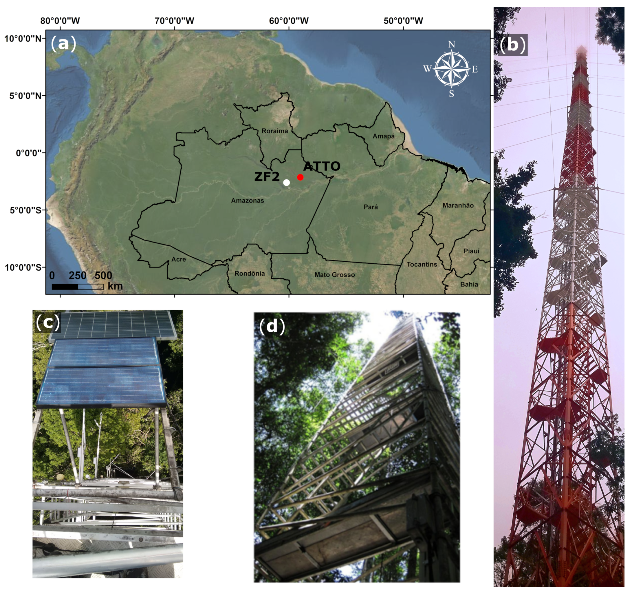
2.1. Experimental Site and Data

The experimental data, collected in micrometeorological towers, used both for the initialization and for the validation of the simulations, are shown in

Table 1. Variables, measurement levels, instrument models and sampling rates used for the ZF2 and ATTO experimental sites.

Variables	Height a.g.l. (m) and Instruments Models	Sampling Rate (Hz)
	ZF2 Tower 1.5, 7.0, 13.5, 18.4, 21.1, 24.5, 31.6, 34.9, 40.4 and 48.2 (CSAT3, Campbell Scientific Inc, Logan, UT. )	20
wind speed components (u, v, w)	ATTO Tower 80 m 14, 40 and 55 (CSAT3, Campbell Scientific Inc, Logan, UT.) 21 (Irgason, Campbell Scientific Inc, Logan, UT.) 81 Windmaster, Gill Instruments Limited, Lymington, UK	10
	ATTO Tower 325 m 150 (CSAT3, Campbell Scientific Inc, Logan, UT.) 325 (Irgason, Campbell Scientific Inc, Logan, UT.)	10 and 20
Air temperature and relative humidity	ATTO Tower 80 m 0.4, 1.5, 4.0, 12.0, 26.0, 36.0, 40.0, 55.0, 73.0 and 81.0 Termohygrometer (CS215, Rotronic Measurement Solutions, Switzerland)	1/60

. In addition, radiosonde data from ATTO site [23] were also used to initialize the simulations. The experimental data from the ATTO site were collected during November 2015 as part of the IOP-I (intensive campaign) of ATTO Project in the Uatumã Sustainable Development Reserve (USDR) [23]. The ATTO research Project is a cooperative effort between researchers from Brazil and Germany (https://www.attoproject.org/, accessed on 29 November 2021). The Project was designed to realize a better understanding of the climatological, ecological, biogeochemical and hydrological issues of the Amazon as a regional entity, but from the perspective of global climate change. The ATTO site is located 150 km northeast of Manaus, AM, Brazil, between 2°27${}^{\prime }$–2°4${}^{\prime }$ S and 54°10${}^{\prime }$–58°4${}^{\prime }$ W [23]. Since 2011, an 80-m scaffolding tower (02°08.647${}^{\prime }$ S, 58°59.992${}^{\prime }$ W) at the site has been used for measurements inside and above the canopy. In 2015, the main 325-m steel lattice tower (02°08.752′ S, 59°00.335${}^{\prime }$ W) was erected [47]. The towers are 670 m apart. Full descriptions of the micrometeorological instrumentation can be found in Dias-Junior et al. [23]. Figure 1 shows the locations of the ATTO site and both towers upon which the micrometeorological instruments were installed. ATTO data were used for both the initializations and validations of the simulations.

To date, no leaf area density profile (LAD) is available for the ATTO site. Therefore, in this work the mean LAD profile showed in Marques-Filho et al. [48] (see their Figure 4) for the Cuieiras Reserve (ZF2) was used (02.36° S, 60.12° W). Since both the ZF2 and the ATTO site are located in the State of Amazonas and have forests with similar and spatially homogeneous aerodynamic characteristics [48,49] using LAD obtained by Marques-Filho et al. [48] was considered a reasonable choice. The total leaf area index used here was LAI = 6.1 m${}^2$/m${}^2$, and the canopy mean height $h_c$ = 40 m (see Table 1) was defined based on the location where the LAD, a(z), approached zero. A canopy drag coefficient $C_d=0.15$ was used. This value is inside the frequently used $C_d$ range for the forest ≈ 0.1–0.4 [14,50,51].

PALM simulations were validated against vertical profiles of turbulence statistics obtained at the ATTO and ZF2 sites. The latter is located approximately 60 km northwest of the city of Manaus and approximately 140 km from the ATTO towers. ZF2 covers an area of approximately 22,700 ha of dense, terra firme, humid tropical forest, typical of central Amazonia [48]. The ZF2 data used here was collected during the GoAmazon 2014–15 project [52]. At ZF2, most measurements occurred inside the canopy (Table 1), whereas at the ATTO site, most measurement levels are above the canopy. To maximize the number of data above and within the forest, experimental profiles from the two sites were used. Both sites are located on plateaus. ZF2 tower sits on a hill 50 m high. The ATTO towers are located on a hill 70 m high [24]. The canopy heights at the ZF2 and ATTO sites were estimated to be 35 m [52] and 37 m [53], respectively.

2.2. Canopy Structure/Model Description

The PALM version used in our simulations was developed by Raasch and Schröter [54] and modified by Maronga et al. [55,56]. It was developed by the Institute of Meteorology and Climatology of Leibniz University, Hannover, Germany. In general, LES models are based on the spatial average of the turbulent fluctuations, which are divided into large scale and small-scale eddies using a specified filter function [57]. The large-scale eddies are then directly simulated, while the small-scale eddies are parameterized (for more details on the basic governing equations for the PALM, see Maronga et al. [55,56]. Equations for the conservation of mass, energy, and humidity are filtered on the grid size, and the processes of molecular diffusion and radiation are neglected. Discretization in time is achieved using the third-order Runge–Kutta time-stepping scheme [58]. The time steps for both simulations was 1.0 s.

The drag force implemented in PALM is similar to performed by Shaw and Schumann [38] and it was calculated through the $C_d$, LAD, resolved scalar wind speed ($|\overline{\mathbf{u}}|$) and resolved velocity vector in the ($x,y,z$) directions ($\overline{\mathbf{u}}$) [59]:

$$\overline{\mathbf{F}}=-C_d\mathrm{LAD}\left|\overline{\mathbf{u}}\right|\overline{\mathbf{u}},$$

(1)

This force is implemented in the plant canopy model (PCM) module of PALM. The PCM module treats trees as a sink for the moment due to the action of viscous forces, as proposed by Shaw and Schumann [38] and Watanabe [60]. This approach assumes that the turbulent kinetic energy sub-grid (SGS-TKE) is dissipated inside the canopy [61]. Other parameterizations to estimate the drag force imposed by the forest canopy can be found in the work carried out by Chen et al. [17].

Another aspect of the canopy is its performance as a heat source. It is known that solar radiation is attenuated as it penetrates the interior of the canopy, with little radiation reaching the ground. The intensity of this attenuation will depend on the LAD [62].

The parameters related to the implementation of the canopy and the computational domain are shown in

Table 2. Model input parameters.

Variable	Símbolo	Value
Horizontal domain size (km)	$Lx$, $Ly$	$4.0\times 4.0$
Domain height (km)	$Lz$	1.6
Grid resolution (m)	$dx$, $dy$, $dz$	20 × 20 × 4
Time step (s)	$dt$	1.0
Canopy height (m)	h	40
Leaf area index	$LAI$	6.1
Surface temperature (K)	$\theta$	302.38
Surface water vapor (g/kg)	q	18.45
Canopy top heat flux (K/s)	$cthf$	0.1
Surface scalar flux (ppm/s)	$Q{s}_0$	2
Spin up time (s)	-	10,800
Total Simulation time (s)	-	14,400
Canopy drag coefficient	$C_d$	0.15

. The heat flux and surface temperature values correspond to average values from an early morning obtained experimentally during the ATTO IOP-I in November 2015.

Two simulations with the same initial conditions and with different geostrophic wind intensities were performed. In the first simulation, a weak wind (WW, geostrophic wind speed = 2 ms${}^{-1}$) condition was simulated. In the second simulation a strong wind (SW, geostrophic wind speed = 6 ms${}^{-1}$) condition was simulated. Weak wind conditions are very common above the Amazon forest [49], but in the presence of convective systems, the wind speeds increase [28]. Due to the objective of the work, a source of passive scalar was implemented in the lower domain of the simulation inside the canopy. A surface scalar flux was implemented similarly to how Kanani-Shring and Raasch [44] did.

2.3. Initial and Boundary Conditions

The initial and boundary conditions and the external forcings were chosen to generate a planetary boundary layer corresponding to the one characterizing an Amazonian morning convective period. Generally, the sensible turbulent heat flux is low and stability is close to neutrality. For this purpose, experimental mean profiles, corresponding to 0800–0900 local time and obtained through sonic anemometers and radiosonde, were used for the period from 11 to 25 November 2015 (ATTO IOP-I). These data were input into the model as initial conditions (Table 2). The initial vertical profiles of the horizontal wind speed components were considered equal to the values of the geostrophic wind components. The initial vertical profiles of the virtual potential temperature (${\theta }_v$) and water vapor (q) were developed to create a mixed layer (ML). Figure 2 shows the first and last hour of the simulated vertical profiles of horizontal wind speed (U): ${\theta }_v$ and q.

3. Results and Discussion

Initially, the profiles of the wind speed and the turbulent fluxes simulated and obtained experimentally will be compared. Then the concentrations of the scalar within and above the forest canopy for the two simulated conditions will be presented. The experimental profiles used in this work are shown in Figure 3 of Santana et al. [49], which were obtained at the two experimental Amazonian sites (ATTO and ZF2) described in Section 2. The U values simulated by PALM at the canopy top (not shown) were 0.7 and 2.5 ms${}^{-1}$ for WW and SW conditions, respectively. Hence, to be compared with the model outputs, the measured data were divided into two classes, U (for the WW comparison) and U (for the SW comparison).

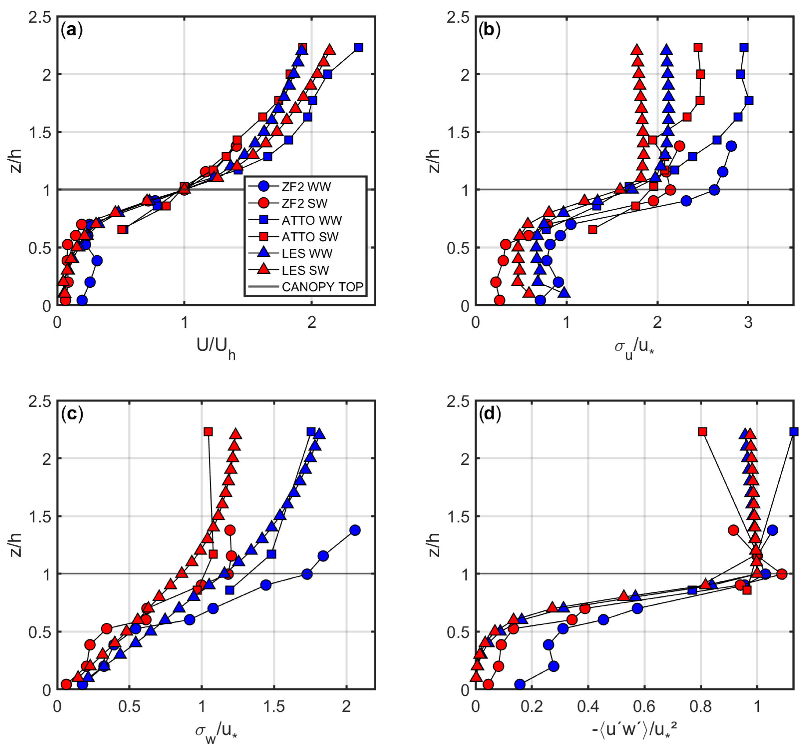
3.1. Simulated and Measured Profiles

The measured and simulated U profiles normalized with the wind speed at the canopy top ${\mathrm{U}}_h$ are depicted in Figure 3a. The standard deviation of the streamwise wind velocity component (${\sigma }_u$) and the standard deviation of the vertical wind velocity component (${\sigma }_w$) normalized by the friction velocity ($u_{*}$), calculated for the canopy top, are depicted in Figure 3b,c. The kinematic momentum fluxes $<u^{\prime }{w}^{\prime }>$ normalized by $u_{*}^2$ are depicted in Figure 3d. The measurement height (z) was normalized by the height of the canopy top (h). The main characteristics observed for both experimental and simulated profiles are: (i) wind speed profiles $\mathrm{U}/{\mathrm{U}}_h$ show an inflection point near the forest–atmosphere interface, with strong attenuation in the wind intensity below 1.0 h. Inflection points are a peculiar characteristic of wind profiles in the forest regions [19,20,63,64]. (ii) ${\sigma }_u/u_{*}$ ${\sigma }_w/u_{*}$ and $<u^{\prime }{w}^{\prime }>/u_{*}^2$ profiles also rapidly decrease with increasing canopy depth. Raupach et al. [19] also noted that $<u^{\prime }{w}^{\prime }>/u_{*}^2$ values tend towards zero close to the ground in response to almost complete horizontal momentum absorption by the canopy [14,19,49].

It is also observed that the experimental and simulated $\mathrm{U}/{\mathrm{U}}_h$ profiles (Figure 3a) present very similar behavior (variation/behavior of the curve) between heights 0.6 and 1.0 $z/h$, and slight differences in the regions above and below this height range. The same is valid for $<u^{\prime }{w}^{\prime }>/u_{*}^2$ profiles. Above the forest, the behavior of the simulated and measured normalized wind profiles are different. At the canopy, the measured profiles show steeper velocity gradients in WW conditions, whereas the LES profiles are steeper in SW profiles. The difference in the wind speed gradient at the canopy top might hint to differences in the shear length scale at the canopy top and to the characteristic of the coherent structures generated at the forest atmosphere interface. The normalized measured and simulated momentum flux profiles close to the ground, $z/h<$ 0.5, show small differences in SW cases and large differences in WW cases. The large differences in the WW cases can be explained by the influence of submeso-structure on the turbulence structure inside the canopy [53]. Above the canopy, the PALM profiles are similar for WW and SW conditions. The measured $<u^{\prime }{w}^{\prime }>/u_{*}^2$ profiles show a tendency to decrease with height in the SW case and to increase with height in the WW case. The former is explained with the weakening of coherent vortices moving away from the canopy top, and the latter is explained by the influence of low frequency processes on the flow.

The experimental and simulated profiles of ${\sigma }_u$ and ${\sigma }_w$ show good agreement in the region comprised between the ground and 0.6 $z/h$. Above this height, the ${\sigma }_w/u_{*}$ simulated values were slightly underestimated compared to the experimental ones. That is evident for both light and strong winds.

The good agreement between the simulated and experimental profiles demonstrates that the model is able to represent well the characteristics of the flow within and above the forest canopy. Santana et al. [49] observed that eddies rarely penetrate deeper forest regions. In this way, an air layer is formed from the ground up to a height of 0.5 $z/h$ that behaves in a decoupled manner from the upper portions, within and above the canopy. This result of segmentation of profile behavior appears well represented in the simulated results, especially for WW simulations.

Figure 4a,b shows the profiles of the variance of the vertical wind velocity component (${\sigma }_w^2$) and the passive scalar concentration (s), respectively. Note that for SW condition, the values of ${\sigma }_w^2$ profile (associate with turbulence intensity) within and above the forest are stronger (higher values of ${\sigma }_w^2$) than for the WW condition. Besides that, the scalar profile for the SW condition shows a smaller gradient between the regions inside and above the canopy forest compared to the WW condition. In the condition of higher turbulence, a smaller gradient of a passive scalar can be observed between the ground and the region above the canopy, which denotes a greater capacity to remove the scalar from the interior of the forest during SW. Between the ground and approximately 0.4 $z/h$, the highest scalar concentration is associated with WW. However, at 0.4 $z/h$ upwards, a reversal occurred, i.e., the higher scalar concentration was associated with SW condition. This result indicates that higher turbulence (strong winds) was associated with higher efficiency in removing the scalar from the ground to higher levels. Kanani-Suhring and Raasch [44], using PALM, showed that LAI and wind velocity influence the scalar concentration inside the forest. Their results showed that the increase in the LAI and the decrease in the wind speed tend to increase the concentration of scalar inside the forest due to the weak vertical wind shear, and consequently the lower turbulent mixing efficiency. The results presented here also show that for lower wind speed the scalar tends to accumulate in lower portions within the forest canopy.

The ${\sigma }_w^2$ profile shows that the turbulent intensity inside the forest is greater for the SW condition. This difference is more pronounced above 0.4 $z/h$, demonstrating the presence of an air layer with distinct behavior of the lower portion [49] and lower efficiency in turbulent mixing for the weak wind condition.

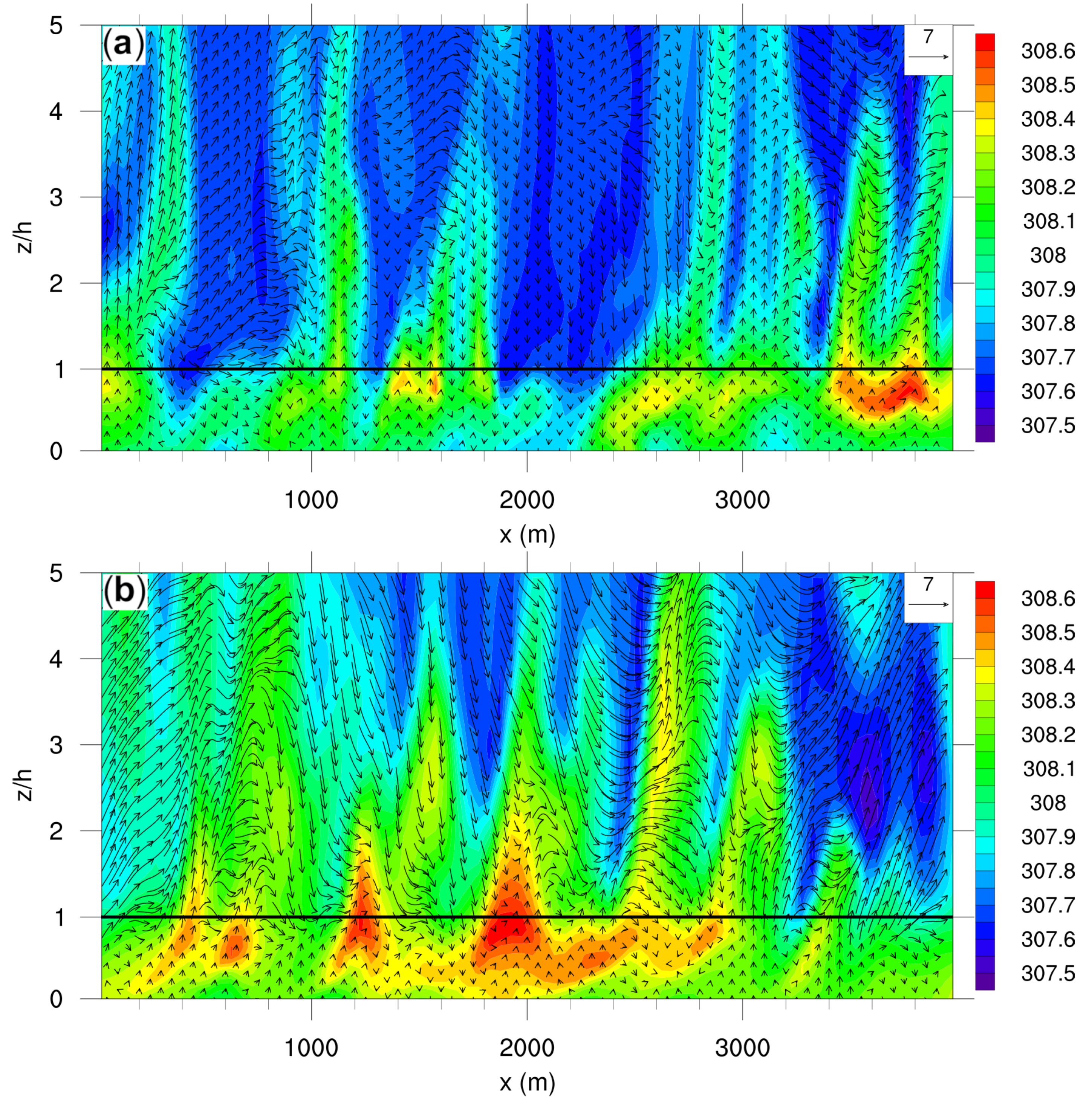
3.2. Temperature and Passive Scalar within and above the Forest Canopy

Figure 5a,b shows the vertical cross-sections of the instantaneous ${\theta }_v$ field for WW and SW conditions, respectively. Note that the highest temperature values are concentrated near the canopy top for both wind conditions, where the LAD is greatest. It can be observed that the region within the canopy presents a more uniform and higher temperature value for SW condition compared to WW condition. Above the canopy, the SW condition shows “plumes” with higher temperatures than the WW condition. These plumes are responsible for the more significant turbulent activity above the canopy, making the turbulent mixing more efficient.

Poggi et al. [65] demonstrated that the lowest region of the forest is dominated by small and weak eddies. At the same time, they emphasized that the canopy top is quite strongly influenced by the turbulent activity above it [66]. In both simulations carried out in this work, the model was able to reproduce the penetration of the turbulent eddies inside the canopy, especially for the strong wind condition. Another highlighted issue is recirculation inside the forest, as described by Cassiani et al. [67]. The flow inside the canopy, promoted by the drainage [68], tends to uniformize the temperature field.

Figure 6a,b shows the zx plane of the passive scalar concentration field for WW and SW conditions, respectively. Note that the highest concentrations of the scalar are located in the region close to the forest ground, for both wind conditions—a result already expected since, it is a region where the source of the scalar was introduced. Comparing the results for both wind conditions, it can be observed that the region inside the canopy presents a lower concentration of the scalar SW condition. Additionally, for the strong wind case, it can be observed that the region above the canopy presents plumes with higher scalar concentrations compared to the WW condition. It can be seen how the plumes formed in the strong wind condition promoted greater mixing and efficiency in removing the scalar from the inside of the forest. This efficiency promotes a decrease in the gradient between the regions within and above the canopy, as shown in Figure 6b.

4. Conclusions

In this work, we investigated the transport of a passive scalar via the PALM model to the Amazon rainforest under two wind conditions: weak (2 ms${}^{-1}$) and strong (6 ms${}^{-1}$). The results showed that the model was able to well reproduce the flow behavior within and above a forest canopy. The average wind profiles, standard deviation and kinematic momentum flux presented a satisfactory comparison with the respective experimental results. The increase in wind speed intensifies the turbulent activity inside the forest and consequently allows more efficient scalar mixing. For situations of weak wind and low turbulence intensity, the simulations highlighted the decoupling of the lower part of the Amazon forest canopy from the atmosphere immediately above. This result was confirmed by several experimental studies. However, for situations of strong winds and intense turbulent activity, a very common situation in the presence of convective clouds, the scalar transport from the interior to the top of the canopy considerably increases, indicating an effective coupling between the flow inside and above the above canopy forest, thereby reducing the scalar gradient.

References

1. Thom, A.; Stewart, J.; Oliver, H.; Gash, J. Comparison of aerodynamic and energy budget estimates of fluxes over a pine forest. Q. J. R. Meteorol. Soc. 1975, 101, 93–105. [Google Scholar] [CrossRef]
2. Högström, U.; Bergström, H. Organized Turbulence Structures in the Near-Neutral Atmospheric Surface Layer. J. Atmos. Sci. 1996, 53, 2452–2464. [Google Scholar] [CrossRef] [Green Version]
3. Simpson, I.; Edwards, G.; Thurtell, G.; Den Hartog, G.; Neumann, H.; Staebler, R. Micrometeorological measurements of methane and nitrous oxide exchange above a boreal aspen forest. J. Geophys. Res. Atmos. 1997, 102, 29331–29341. [Google Scholar] [CrossRef]
4. Zahn, E.; Dias, N.L.; Araújo, A.; Sá, L.D.A.; Sörgel, M.; Trebs, I.; Wolff, S.; Manzi, A. Scalar turbulent behavior in the roughness sublayer of an Amazonian forest. Atmos. Chem. Phys. 2016, 16, 11349–11366. [Google Scholar] [CrossRef] [Green Version]
5. Chor, T.L.; Dias, N.L.; Araújo, A.; Wolff, S.; Zahn, E.; Manzi, A.; Trebs, I.; Sá, M.O.; Teixeira, P.R.; Sörgel, M. Flux-variance and flux-gradient relationships in the roughness sublayer over the Amazon forest. Agric. For. Meteorol. 2017, 239, 213–222. [Google Scholar] [CrossRef]
6. Tajchman, S.J. Comments on measuring turbulent exchange within and above forest canopy. Bull. Am. Meteorol. Soc. 1981, 62, 1550–1559. [Google Scholar] [CrossRef] [Green Version]
7. Blanken, P.; Black, T.A.; Neumann, H.H.; Den Hartog, G.; Yang, P.C.; Nesic, Z.; Staebler, R.; Chen, W.; Novak, M.D. Turbulent Flux Measurements Above and Below the Overstory of a Boreal Aspen Forest. Bound.-Layer Meteorol. 1998, 89, 109–140. [Google Scholar] [CrossRef]
8. Araújo, A.C.; Nobre, A.D.; Kruijt, B.; Elbers, J.A.; Dallarosa, R.; Stefani, P.; von Randow, C.; Manzi, A.O.; Culf, A.D.; Gash, J.H.C.; et al. Comparative measurements of carbon dioxide fluxes from two nearby towers in a central Amazonian rainforest: The Manaus LBA site. J. Geophys. Res. Atmos. 2002, 107, LBA-58. [Google Scholar] [CrossRef] [Green Version]
9. Tóta, J.; Fitzjarrald, D.R.; Staebler, R.M.; Sakai, R.K.; Moraes, O.M.M.; Acevedo, O.C.; Wofsy, S.C.; Manzi, A.O. Amazon rain forest subcanopy flow and the carbon budget: Santarém LBA-ECO site. J. Geophys. Res. Biogeosci. 2008, 113, G00B02. [Google Scholar] [CrossRef]
10. Katul, G.G.; Oren, R.; Manzoni, S.; Higgins, C.; Parlange, M.B. Evapotranspiration: A process driving mass transport and energy exchange in the soil-plant-atmosphere-climate system. Rev. Geophys. 2012, 50. [Google Scholar] [CrossRef] [Green Version]
11. Dias-Júnior, C.Q.; Sá, L.D.; Filho, E.P.M.; Santana, R.A.; Mauder, M.; Manzi, A.O. Turbulence regimes in the stable boundary layer above and within the Amazon forest. Agric. For. Meteorol. 2017, 233, 122–132. [Google Scholar] [CrossRef]
12. Dupont, S.; Brunet, Y. Influence of foliar density profile on canopy flow: A large-eddy simulation study. Agric. For. Meteorol. 2008, 148, 976–990. [Google Scholar] [CrossRef]
13. Patton, E.G.; Katul, G.G. Turbulent pressure and velocity perturbations induced by gentle hills covered with sparse and dense canopies. Bound.-Layer Meteorol. 2009, 133, 189–217. [Google Scholar] [CrossRef]
14. Dias-Júnior, C.Q.; Marques Filho, E.P.; Sá, L.D. A large eddy simulation model applied to analyze the turbulent flow above Amazon forest. J. Wind Eng. Ind. Aerodyn. 2015, 147, 143–153. [Google Scholar] [CrossRef]
15. Kanani-Sühring, F.; Raasch, S. Enhanced scalar concentrations and fluxes in the lee of forest patches: A large-eddy simulation study. Bound.-Layer Meteorol. 2017, 164, 1–17. [Google Scholar] [CrossRef]
16. Liu, Z.; Ishihara, T.; He, X.; Niu, H. LES study on the turbulent flow fields over complex terrain covered by vegetation canopy. J. Wind Eng. Ind. Aerodyn. 2016, 155, 60–73. [Google Scholar] [CrossRef]
17. Chen, X.; Massman, W.J.; Su, Z. A column canopy-air turbulent diffusion method for different canopy structures. J. Geophys. Res. Atmos. 2019, 124, 488–506. [Google Scholar] [CrossRef]
18. Chen, B.; Chamecki, M.; Katul, G.G. Effects of Gentle Topography on Forest-Atmosphere Gas Exchanges and Implications for Eddy-Covariance Measurements. J. Geophys. Res. Atmos. 2020, 125. [Google Scholar] [CrossRef]
19. Raupach, M.R.; Finnigan, J.J.; Brunei, Y. Coherent eddies and turbulence in vegetation canopies: The mixing-layer analogy. Bound.-Layer Meteorol. 1996, 78, 351–382. [Google Scholar] [CrossRef]
20. de Souza, C.M.; Dias-Júnior, C.Q.; Tóta, J.; de Abreu Sá, L.D. An empirical-analytical model of the vertical wind speed profile above and within an Amazon forest site. Meteorol. Appl. 2016, 23, 158–164. [Google Scholar] [CrossRef] [Green Version]
21. Robinson, S.K. Coherent Motions in the Turbulent Boundary Layer. Annu. Rev. Fluid Mech. 1991, 23, 601–639. [Google Scholar] [CrossRef]
22. Katul, G.; Kuhn, G.; Schieldge, J.; Hsieh, C.I. The ejection-sweep character of scalar fluxes in the unstable surface layer. Bound.-Layer Meteorol. 1997, 83, 1–26. [Google Scholar] [CrossRef]
23. Dias-Júnior, C.Q.; Dias, N.L.; dos Santos, R.M.N.; Sörgel, M.; Araújo, A.; Tsokankunku, A.; Ditas, F.; de Santana, R.A.; Von Randow, C.; Sá, M.; et al. Is there a classical inertial sublayer over the Amazon forest? Geophys. Res. Lett. 2019, 46, 5614–5622. [Google Scholar] [CrossRef]
24. Chamecki, M.; Freire, L.S.; Dias, N.L.; Chen, B.; Dias-Junior, C.Q.; Toledo Machado, L.A.; Sörgel, M.; Tsokankunku, A.; Araújo, A.C. Effects of vegetation and topography on the boundary layer structure above the Amazon forest. J. Atmos. Sci. 2020, 77, 2941–2957. [Google Scholar] [CrossRef]
25. Warhaft, Z. Passive Scalars in Turbulent Flows. Annu. Rev. Fluid Mech. 2000, 32, 203–240. [Google Scholar] [CrossRef]
26. Betts, A.K. Transport of ozone to the surface by convective downdrafts at night. J. Geophys. Res. 2002, 107, LBA-13. [Google Scholar] [CrossRef]
27. Gerken, T.; Wei, D.; Chase, R.J.; Fuentes, J.D.; Schumacher, C.; Machado, L.A.; Andreoli, R.V.; Chamecki, M.; de Souza, R.A.F.; Freire, L.S.; et al. Downward transport of ozone rich air and implications for atmospheric chemistry in the Amazon rainforest. Atmos. Environ. 2016, 124, 64–76. [Google Scholar] [CrossRef] [Green Version]
28. Dias-Júnior, C.Q.; Dias, N.L.; Fuentes, J.D.; Chamecki, M. Convective storms and non-classical low-level jets during high ozone level episodes in the Amazon region: An ARM/GOAMAZON case study. Atmos. Environ. 2017, 155, 199–209. [Google Scholar] [CrossRef] [Green Version]
29. Melo, A.M.; Dias-Junior, C.Q.; Cohen, J.C.; Sá, L.D.; Cattanio, J.H.; Kuhn, P.A. Ozone transport and thermodynamics during the passage of squall line in Central Amazon. Atmos. Environ. 2019, 206, 132–143. [Google Scholar] [CrossRef]
30. Zhuang, Y.; Amiro, B.D. Pressure Fluctuations during Coherent Motions and Their Effects on the Budgets of Turbulent Kinetic Energy and Momentum Flux within a Forest Canopy. J. Appl. Meteorol. Climatol. 1994, 33, 704–711. [Google Scholar] [CrossRef] [Green Version]
31. Burns, S.P.; Sun, J.; Lenschow, D.H.; Oncley, S.P.; Stephens, B.B.; Yi, C.; Anderson, D.E.; Hu, J.; Monson, R.K. Atmospheric stability effects on wind fields and scalar mixing within and just above a subalpine forest in sloping terrain. Bound.-Layer Meteorol. 2011, 138, 231–262. [Google Scholar] [CrossRef] [Green Version]
32. Cava, D.; Katul, G. On the scaling laws of the velocity-scalar cospectra in the canopy sublayer above tall forests. Bound.-Layer Meteorol. 2012, 145, 351–367. [Google Scholar] [CrossRef]
33. Foken, T.; Aubinet, M.; Leuning, R. The eddy covariance method. In Eddy Covariance; Springer: Berlin/Heidelberg, Germany, 2012; pp. 1–19. [Google Scholar]
34. Miranda, F.O.; Ramos, F.M.; von Randow, C.; Dias-Júnior, C.Q.; Chamecki, M.; Fuentes, J.D.; Manzi, A.O.; de Oliveira, M.E.; de Souza, C.M. Detection of extreme phenomena in the stable boundary layer over the Amazonian forest. Atmosphere 2020, 11, 952. [Google Scholar] [CrossRef]
35. Aubinet, M. Eddy covariance CO2 flux measurements in nocturnal conditions: An analysis of the problem. Ecol. Appl. 2008, 18, 1368–1378. [Google Scholar] [CrossRef]
36. Katul, G.; Finnigan, J.; Poggi, D.; Leuning, R.; Belcher, S. The influence of hilly terrain on canopy-atmosphere carbon dioxide exchange. Bound.-Layer Meteorol. 2006, 118, 189–216. [Google Scholar] [CrossRef]
37. Belcher, S.E.; Harman, I.N.; Finnigan, J.J. The wind in the willows: Flows in forest canopies in complex terrain. Annu. Rev. Fluid Mech. 2012, 44, 479–504. [Google Scholar] [CrossRef]
38. Shaw, R.H.; Schumann, U. Large-eddy simulation of turbulent flow above and within a forest. Bound.-Layer Meteorol. 1992, 61, 47–64. [Google Scholar] [CrossRef] [Green Version]
39. Kanda, M.; Hino, M. Organized structures in developing turbulent flow within and above a plant canopy, using a large eddy simulation. Bound.-Layer Meteorol. 1994, 68, 237–257. [Google Scholar] [CrossRef]
40. Finnigan, J.J.; Shaw, R.H.; Patton, E.G. Turbulence structure above a vegetation canopy. J. Fluid Mech. 2009, 637, 387–424. [Google Scholar] [CrossRef] [Green Version]
41. Dupont, S.; Brunet, Y. Coherent structures in canopy edge flow: A large-eddy simulation study. J. Fluid Mech. 2009, 630, 93–128. [Google Scholar] [CrossRef]
42. Shaw, R.H.; Patton, E.G.; Finnigan, J.J. Coherent Eddy Structures Over Plant Canopies. In Coherent Flow Structures at Earth’s Surface; John Wiley & Sons, Ltd.: Hoboken, NJ, USA, 2013; Chapter 10; pp. 149–159. [Google Scholar] [CrossRef]
43. Patton, E.G.; Sullivan, P.P.; Shaw, R.H.; Finnigan, J.J.; Weil, J.C. Atmospheric stability influences on coupled boundary layer and canopy turbulence. J. Atmos. Sci. 2016, 73, 1621–1647. [Google Scholar] [CrossRef]
44. Kanani-Sühring, F.; Raasch, S. Spatial variability of scalar concentrations and fluxes downstream of a clearing-to-forest transition: A large-eddy simulation study. Bound.-Layer Meteorol. 2015, 155, 1–27. [Google Scholar] [CrossRef]
45. Neves, T.; Fisch, G.; Raasch, S. Local Convection and Turbulence in the Amazonia Using Large Eddy Simulation Model. Atmosphere 2018, 9, 399. [Google Scholar] [CrossRef] [Green Version]
46. Carneiro, R.; Fisch, G.; Neves, T.; Santos, R.; Santos, C.; Borges, C. Nocturnal Boundary Layer Erosion Analysis in the Amazon Using Large-Eddy Simulation during GoAmazon Project 2014/5. Atmosphere 2021, 12, 240. [Google Scholar] [CrossRef]
47. Andreae, M.O.; Acevedo, O.C.; Araùjo, A.; Artaxo, P.; Barbosa, C.G.G.; Barbosa, H.M.J.; Brito, J.; Carbone, S.; Chi, X.; Cintra, B.B.L.; et al. The Amazon Tall Tower Observatory (ATTO): Overview of pilot measurements on ecosystem ecology, meteorology, trace gases, and aerosols. Atmos. Chem. Phys. 2015, 15, 10723–10776. [Google Scholar] [CrossRef] [Green Version]
48. Marques Filho, A.D.O.; Dallarosa, R.G.; Pachêco, V.B. Radiação solar e distribuição vertical de área foliar em floresta–Reserva Biológica do Cuieiras–ZF2, Manaus. Acta Amazon. 2005, 35, 427–436. [Google Scholar] [CrossRef]
49. Santana, R.A.; Dias-Júnior, C.Q.; Tóta, J.; Fuentes, J.D.; do Vale, R.S.; Alves, E.G.; dos Santos, R.M.N.; Manzi, A.O. Air turbulence characteristics at multiple sites in and above the Amazon rainforest canopy. Agric. For. Meteorol. 2018, 260–261, 41–54. [Google Scholar] [CrossRef]
50. Katul, G.G.; Mahrt, L.; Poggi, D.; Sanz, C. One-and two-equation models for canopy turbulence. Bound.-Layer Meteorol. 2004, 113, 81–109. [Google Scholar] [CrossRef] [Green Version]
51. Queck, R.; Bienert, A.; Maas, H.G.; Harmansa, S.; Goldberg, V.; Bernhofer, C. Wind fields in heterogeneous conifer canopies: Parameterisation of momentum absorption using high-resolution 3D vegetation scans. Eur. J. For. Res. 2012, 131, 165–176. [Google Scholar] [CrossRef]
52. Fuentes, J.D.; Chamecki, M.; dos Santos, R.M.N.; Randow, C.V.; Stoy, P.C.; Katul, G.; Fitzjarrald, D.; Manzi, A.; Gerken, T.; Trowbridge, A.; et al. Linking Meteorology, Turbulence, and Air Chemistry in the Amazon Rain Forest. Bull. Am. Meteorol. Soc. 2016, 97, 2329–2342. [Google Scholar] [CrossRef]
53. Oliveira, P.E.S.; Acevedo, O.C.; Sörgel, M.; Tsokankunku, A.; Wolff, S.; Araújo, A.C.; Souza, R.A.F.; Sá, M.O.; Manzi, A.O.; Andreae, M.O. Nighttime wind and scalar variability within and above an Amazonian canopy. Atmos. Chem. Phys. 2018, 18, 3083–3099. [Google Scholar] [CrossRef] [Green Version]
54. Raasch, S.; Schröter, M. PALM-A large-eddy simulation model performing on massively parallel computers. Meteorol. Z. 2001, 10, 363–372. [Google Scholar] [CrossRef]
55. Maronga, B.; Gryschka, M.; Heinze, R.; Hoffmann, F.; Kanani-Sühring, F.; Keck, M.; Ketelsen, K.; Letzel, M.O.; Sühring, M.; Raasch, S. The Parallelized Large-Eddy Simulation Model (PALM) version 4.0 for atmospheric and oceanic flows: Model formulation, recent developments, and future perspectives. Geosci. Model Dev. 2015, 8, 2515–2551. [Google Scholar] [CrossRef] [Green Version]
56. Maronga, B.; Banzhaf, S.; Burmeister, C.; Esch, T.; Forkel, R.; Fröhlich, D.; Fuka, V.; Gehrke, K.F.; Geletič, J.; Giersch, S.; et al. Overview of the PALM model system 6.0. Geosci. Model Dev. 2020, 13, 1335–1372. [Google Scholar] [CrossRef]
57. Pope, S.B.; Pope, S.B. Turbulent Flows; Cambridge University Press: Cambridge, UK, 2000. [Google Scholar]
58. Williamson, J. Low-storage Runge–Kutta schemes. J. Comput. Phys. 1980, 35, 48–56. [Google Scholar] [CrossRef]
59. Patton, E.G.; Sullivan, P.P.; Davis, K.J. The influence of a forest canopy on top-down and bottom-up diffusion in the planetary boundary layer. Q. J. R. Meteorol. Soc. 2003, 129, 1415–1434. [Google Scholar] [CrossRef]
60. Watanabe, T. Large-eddy simulation of coherent turbulence structures associated with scalar ramps over plant canopies. Bound.-Layer Meteorol. 2004, 112, 307–341. [Google Scholar] [CrossRef]
61. Shaw, R.H.; Patton, E.G. Canopy element influences on resolved- and subgrid-scale energy within a large-eddy simulation. Agric. For. Meteorol. 2003, 115, 5–17. [Google Scholar] [CrossRef] [Green Version]
62. Brown, K.W.; Covey, W. The energy-budget evaluation of the micrometeorological transfer processes within a cornfield. Agric. Meteorol. 1966, 3, 73–96. [Google Scholar] [CrossRef]
63. Finnigan, J. Turbulence in Plant Canopies. Annu. Rev. Fluid Mech. 2000, 32, 519–571. [Google Scholar] [CrossRef]
64. Dias-Júnior, C.; Sá, L.; Pachêco, V.; de Souza, C. Coherent structures detected in the unstable atmospheric surface layer above the Amazon forest. J. Wind. Eng. Ind. Aerodyn. 2013, 115, 1–8. [Google Scholar] [CrossRef]
65. Poggi, D.; Porporato, A.; Ridolfi, L.; Albertson, J.D.; Katul, G.G. The Effect of Vegetation Density on Canopy Sub-Layer Turbulence. Bound.-Layer Meteorol. 2004, 111, 565–587. [Google Scholar] [CrossRef]
66. Dwyer, M.J.; Patton, E.G.; Shaw, R.H. Turbulent kinetic energy budgets from a large-eddy simulation of airflow above and within a forest canopy. Bound.-Layer Meteorol. 1997, 84, 23–43. [Google Scholar] [CrossRef]
67. Cassiani, M.; Katul, G.; Albertson, J. The effects of canopy leaf area index on airflow across forest edges: Large-eddy simulation and analytical results. Bound.-Layer Meteorol. 2008, 126, 433–460. [Google Scholar] [CrossRef] [Green Version]
68. Tota, J.; Roy Fitzjarrald, D.; da Silva Dias, M.A. Amazon rainforest exchange of carbon and subcanopy air flow: Manaus LBA site—A complex terrain condition. Sci. World J. 2012, 2012, 165067. [Google Scholar] [CrossRef] [PubMed] [Green Version]
Figure 1. (a) Localizations of the ZF2 and ATTO sites. (b) Ground view of the 325 m ATTO tower. (c) View from the top of the ZF2 site tower. (d) Ground view of the 80 m ATTO tower.
Atmosphere 12 01631 g001
Figure 2. Initial vertical profiles of: (a) horizontal wind speed (U); (b) virtual potential temperature ( θ v ); (c) water vapor (q). FT LES WW and FT LES SW are the mean profiles of the first hour of the simulation for WW and SW conditions, respectively. LT LES WW and LT LES SW are the mean profiles of the last hour of the simulation for WW and SW conditions, respectively.
Atmosphere 12 01631 g002
Figure 3. Normalized vertical profiles of: (a) the mean wind speed ( U / U h ); (b) the standard deviation of the horizontal wind speed ( σ u / u * ); (c) the standard deviation of the vertical wind speed ( σ w / u * ); (d) kinematic momentum flux ( < u w > / u * 2 ). U h is the wind speed calculated at canopy top; h is the height of the canopy; u * is the friction velocity calculated at the canopy top. The horizontal black line at z / h = 1 indicates the canopy top.
Atmosphere 12 01631 g003
Figure 4. Vertical profiles of: (a) the variance of the vertical wind velocity ( σ w 2 ); (b) the passive scalar concentration (s). The horizontal black line at z / h = 1 marks the height of the canopy.
Atmosphere 12 01631 g004
Figure 5. Virtual Potential Temperature simulated zx planes ( θ v ): (a) weak wind condition; (b) strong wind condition. The color scale represents the values of θ v in Kelvin. The horizontal black line represents the height of the canopy. The heights (z) were normalized by the height of the canopy (h). The y-position of the cutting plane is 2000 m.
Atmosphere 12 01631 g005
Figure 6. Passive scalar concentration simulated zx planes (s). (a) Weak wind condition; (b) Strong wind condition. The color scale represents the values of s 1 / 3 in ppm. The horizontal black line represents the height of the canopy. The heights (z) were normalized by the height of the canopy (h). The position in y of the cutting planes is 2000 m.
Atmosphere 12 01631 g006