Raindrop Size Distribution and Rain Characteristics of the 2017 Great Hunan Flood Observed with a Parsivel² Disdrometer

Abstract

Disdrometer observations obtained by an OTT Parsivel² during the 2017 Great Hunan Flood from 1:00 a.m. LST 23 June 2017 to 4:00 a.m. LST 2 July 2017 in Changsha, Hunan Province, southern China, are analyzed to diagnose characteristics of raindrop size distribution (DSD). This event was characterized by a large number of small- to medium-sized raindrops (diameters smaller than 1.5 mm) and the mean median volume diameter (D₀) is about 1.04 mm. The median values of rain rate R (1.57 mm h⁻¹), liquid water content W (0.10 g m⁻³), and radar reflectivity Z (25.7 dBZ) are smaller than that of the 2013 Great Colorado Flood. This event was composed of two intense rainfall periods and a stratiform period, and notable distinctions of rainfall microphysics among the three rainfall episodes are observed. Two intense rainfall periods were characterized by widespread and intense convection rains with a surface reflectivity of 48.8~56.7 dBZ. A maximum diameter of raindrops up to 7.5 mm was observed, as well as high concentrations of small and midsize drops, resulting in large rainfall amounts during the two intense rainfall episodes. The mean radar reflectivity of 22.6 dBZ, total rainfall of 17.85 mm and the maximum raindrop of approximately 4.25 mm were observed during the stratiform rainfall episode. The composite DSD for each rainfall episode peaked at 0.56 mm but higher concentrations of raindrops appeared in the two intense rainfall episodes. The Z-R relationships derived from the disdrometer measurements reflect the unusual characteristics of DSD during the flood. As a result, the standard NEXRAD Z-R relationship (Z = 300R^1.4) strongly underestimated hourly rainfall by up to 27.5%. In addition, the empirical relations between rainfall kinetic energy (KE) versus rainfall intensity (R) and mean mass diameter (D_m) are also derived using DSDs to further investigate the impacts of raindrop properties on the rainfall erosivity.

1. Introduction

Persistent heavy rainfall (PHR) events such as the 2017 Great Hunan Flood are characterized by several observable attributes: high intensity, wide range, long duration, and strong stability [1]. Once the PHR event occurs, it often tends to cause flood disasters and huge economic losses due to the difficulty of accurate weather forecasting, which severely threatens human life and property. Hunan, located in the East Asian monsoon climate zone, is one of the provinces with frequent PHR events in China. During the period of 22 June to 2 July 2017, a large area of heavy rainfall with maximum local amounts approximatively 576 mm fell over Hunan Province and adjacent regions, affecting a total of 4,030,700 people and a direct economic loss of ¥6.014 billion, according to the official report. This heavy a rainstorm, which had not been witnessed in this region for several decades, was characterized by its long duration, widespread flooding, and intense precipitation. Extreme hydrometeorological events are difficult to forecast, since their weather patterns and the related microphysical processes within the models do not resemble the standard conditions of a region for which forecasting and nowcasting systems may have been tuned [2]. Therefore, it is necessary to study extreme typical heavy precipitation event like the 2017 Great Hunan Flood from multiple perspectives to improve our understanding of such PHR events.

Several studies have mainly focused on the meteorological and hydrological settings on a large spatial scale as well as the temporal and spatial distribution of rainfall. Jin et al. [3] concluded that the stable maintenance of upper-level cold vortex and the subtropical high over Hunan province provides favorable large-scale circulation conditions for the occurrence of this type of heavy rainfall. Chen et al. [4] analyzed the circulation background and the transportation of the large-scale water vapor during the 2017 great Hunan flood using the NCEP/NCAR reanalysis data and found that sufficient water vapors from the Indian Ocean and the South China Sea entered Hunan Province with the convergence of airflow at the lower level and aggregated and condensed in the middle- and upper- level through the strong vertical upward movements, leading to the intense precipitation. Li et al. [5] stressed the importance of the moisture divergence vertical flux and thermodynamic wave activity density in the diagnosis and prediction of severe rainstorms from the NCEP/NCAR Global Forecasting System (GFS) model.

These studies listed above explained the main driving mechanisms for the distribution, amount, and vertical structure of clouds as well as precipitation on a mesoscale during the 2017 Great Hunan Flood. In contrast, the spatial and temporal evolution of raindrop size distribution (DSD) and rain characteristics (i.e., rainfall intensity, mean diameter, and number concentration) that vary at a scale very smaller than the model resolution only received minimal investigation and remain largely unknown [6]. The formation of precipitation involves not only dynamics and thermodynamics but also microphysical processes. The raindrop is the final form of liquid precipitation, and DSD is the number of raindrops per unit volume per mm interval of the diameter, which evolves with precipitation both in time and space. The characteristics of DSD are related to multiple complex microphysical and dynamic processes, like collision-coalescence, breakup, and evaporation [7]. Rainfall parameters such as rain rate (R: mm h⁻¹), radar reflectivity (Z: dBZ) and liquid water content (W: g m⁻³) can be calculated from the DSD once it is known. In addition, the knowledge of DSD is also required for the radar quantitative precipitation estimation (QPE), satellite retrieval of precipitation, microphysics parameterization in numerical weather prediction models and soil erosivity estimation [8,9,10,11,12]. Therefore, this work aims to contribute to the understanding of the microphysical properties of the 2017 Great Hunan Flood by using the consecutive eleven-day measurements of the OTT Parsivel² disdrometer from 22 June to 2 July 2017, when the rainbands passed over the Changsha site. On a wider scope, this paper not only gives an insight into the microphysical features of an extreme hydrometeorological event that occurred in southern China, but also contributes to the precipitation microphysical studies on regional or global scales, as well as remote sensing measurement of precipitation.

To facilitate the detailed analysis of the microphysical characteristics of rainfall, this rainfall process was divided into three rainfall episodes, since the duration of this flood event was so long. Total rainfall amounts, DSDs, rainfall characteristics (mean mass-weighted diameter D_m, and normalized intercept parameter N_w) and the Z-R and KE-R relationships observed during the three rainfall episodes are compared and analyzed with respect to the microphysical processes. For the entire rainfall period, the characteristics of DSD in different rain rate classes, the percentage of occurrence, amount of rainfall and percentage of contribution to the total rainfall for each rain rate category were computed. Moreover, the performance of hourly rainfall estimations of the NEXRAD Z-R relationship was also examined.

2. Data and Methods

2.1. Instruments and Dataset

The data sets used in this study were collected by a second-generation OTT Parsivel² disdrometer at a national weather station in Changsha (CS) City, Hunan Province, from 22 June to 2 July 2017. Changsha, a provincial capital city in Hunan Province located in the southeast of China, is strongly influenced by the subtropical continental monsoon in summer and is an inland region that features plains and hills. A topographic map of the field site (CS site: 28.11°N, 112.79°E) is shown in Figure 1a. The Parsivel² disdrometer (Figure 1b) operated by Changsha Meteorological Bureau was deployed within the local observation station and the optional S-band weather radar in Changsha is ~5 km northeast of the CS site. This radar applied a standard WSR-88D scanning strategy and consists of 14 or 15 elevation angle scans ranging from 0.5° to 19.5°. In addition, 3543 ground gauges were used to analyze the spatial distribution of rainfall (not shown).

The OTT Parsivel² is a laser-optical disdrometer with a horizontal laser beam of 54 cm² that provides the number of raindrops in 32 bins of diameters from 0 to 25 mm and fall speeds from 0 to 22.4 m s⁻¹. A more detailed description of the OTT Parsivel² device can be found in Löffler-Mang and Joss [13]. The lowest two size classes are not used because of the poor reliability of their low signal-to-noise ratio. Thus, the smallest size of raindrops was limited to approximately 0.312 mm. Also, the measured maximum diameter could reach about eight mm because of the break-up of larger raindrops during the falling.

In this study the temporal resolution was 1 min. To identify and remove suspicious measurements (due to turbulence, splashing, multiple drops at a time, margin fallers, insects, spiders, etc.), a fall velocity-based filter was applied to the raw Parsivel² measurements (32 × 32 drop counts) [14]. Namely, only drops that have the measured velocity satisfying the equation:

$$\left|v{\left(\mathrm{D}\right)}_{\mathrm{Meas}}-v{\left(\mathrm{D}\right)}_{\mathrm{Brandes}}\right|\le 0.6v{\left(\mathrm{D}\right)}_{\mathrm{Brandes}}$$

(1)

are considered, where v(D)_Meas is the velocity measured by Parsivel², and v(D)_Brandes is the velocity for a drop of diameter D according to the velocity-diameter relationship proposed by Brandes et al. (2002) [15]. As shown in Figure 2, the distribution of raindrop numbers is almost entirely within the ±60% of the empirical velocity model of Brandes et al. [15] despite that the Parsivel² lightly underestimated the mean fall velocity of the raindrops in classes with diameters from 1.375 to 2.75 mm and overestimated the fall velocity of the drops at sizes larger than 5.5 mm. In terms of rain amount, the filtered drops occupied only 1.1% of the total rain amount. Note that if the 1-min DSD sample with a total number of drops is lesser than 10 or a DSD-derived rain rate is lower than 0.1 mm h⁻¹, it is also regarded as noise and not considered to be a rainy minute. After all the quality control (QC) criteria above, 7062 1-min DSD samples remaining were used in the following analysis.

2.2. Comparison with Rain Gauges

Four different rainfall statistics: correlation coefficient (CC), root mean square error (RMSE), normalized absolute error (NE), and bias were employed to quantify the results for the comparative study in this paper, and they are defined as:

$$\mathrm{CC}=\frac{{\displaystyle \sum _{i=1}^N(X_i-\overline{X})}(Y_i-\overline{Y})}{\sqrt{{\displaystyle \sum _{i=1}^N(X_i-\overline{X})}}\sqrt{{\displaystyle \sum _{i=1}^N(Y_i-\overline{Y})}}}$$

(2)

$$\mathrm{RMSE}={\left[\frac{1}{N}{\displaystyle \sum _{i=1}^N{(X_i-Y_i)}^2}\right]}^{1/2}$$

(3)

$$\mathrm{NE}=\frac{\frac{1}{N}{\displaystyle \sum _{i=1}^N\left|X_i-Y_i\right|}}{\overline{Y}}$$

(4)

$$\mathrm{Bias}=\frac{{\displaystyle \sum _{i=1}^N\left(X_i-Y_i\right)}}{{\displaystyle \sum _{i=1}^N{Y}_i}}\times 100\%$$

(5)

where N is the total number of samples, X and Y represent the estimated variable and reference variable, respectively. The symbol “¯” in Equation (2) represents the sample average.

The measurements from a rain gauge next to the Parsivel² (Figure 1b) are accepted as the official observations after quality control from the Parsivel². Figure 3 shows the inter-comparison of hourly rainfall between Parsivel² and the rain gauge. Excellent agreement is found, with a correlation coefficient of 0.98 between two independent instruments with negligible aberrations. In addition, the Parsivel² shows 9.66% less hourly rainfall than the rain gauge, which is in a relatively lower deviation than that reported in the previous studies [16]. The slightly underestimation of hourly rainfall observed from Parsivel² is believed to be a manifestation of small particle detection issues [17].

2.3. Raindrop Size Distribution

In order to investigate the characteristics of precipitation, DSD and its derived bulk properties are calculated from the following formulas. In this study, measured DSD is calculated from the number of drops (n_ij) recorded by the Parsivel² at the ith size and jth velocity bin:

$$N(D_{\mathrm{i}})={\displaystyle \sum _{\mathrm{j}=1}^{32}\frac{n_{ij}}{A\Delta t{V}_j\Delta D_i}}$$

(6)

where N(D_i) (mm⁻¹m⁻³) is the number concentration of drops within diameters in the interval from D_i to D_i + ΔD_i per unit size interval; D_i (mm) is equivalent spherical raindrop diameter of the ith size bin and ΔD_i (mm) is the corresponding diameter interval; A (m²) and Δt (s) are the effective instrument sample area and time interval, respectively; V_j (m s⁻¹) is the fall speed for the velocity bin j.

Given N (D_i), the integral rainfall quantities viz. radar reflectivity Z (mm⁶ m⁻³), rain rate R (mm h⁻¹), liquid water content W (g m⁻³), and the total number concentration of raindrop N_t (m⁻³), can be derived as follows:

$$\mathrm{Z}={\displaystyle \sum _{i=1}^{32}N(D_i)D_i^6}\Delta D_i$$

(7)

$$\mathrm{R}=\frac{6\pi }{{10}^4}{\displaystyle \sum _{i=1}^{32}{\displaystyle \sum _{j=1}^{32}{V}_{j}N(D_i)D_i^3}\Delta D_i}$$

(8)

$$\mathrm{W}=\frac{\pi }{6\times {10}^3}{\displaystyle \sum _{i=1}^{32}N(D_i)D_i^3}\Delta D_i$$

(9)

$$N_t={\displaystyle \sum _{i=1}^{32}N(D_i)}\Delta D_i$$

(10)

The well-known three-parameter gamma model DSD [18] is used in this study:

$$N(D)=N_0{D}^{\mu }{e}^{-\Lambda D}$$

(11)

where D (mm) is the raindrop diameter, N₀ (mm^−1-μm⁻³) is the intercept parameter, μ (dimensionless) and Λ (mm⁻¹) are the shape and slope parameters, respectively. The nth-order moment of a DSD, M_n, is expressed as:

$$M_n={\displaystyle {\int }_0^{D_{\max }}N(D)D^{n}dD}$$

(12)

The mass-weight mean diameter D_m (mm) and the generalized intercept parameter N_w (m⁻³ mm⁻¹) were calculated as:

$$D_m=\frac{M_4}{M_3}=\frac{{\displaystyle \sum _{i=1}^{32}N(D_i)D_i^4}\Delta D_i}{{\displaystyle \sum _{i=1}^{32}N(D_i)D_i^3}\Delta D_i}$$

(13)

$$N_w=\frac{4^4}{\pi {\mathsf{\rho }}_w}\left(\frac{{10}^{3}W}{D_m^4}\right)$$

(14)

where M₄ and M₃ are the 4th-order and 3rd-order moment of the DSD, respectively. ρ_w (1.0 g cm⁻³) is the density of water. Note that the derived DSD parameters (e.g., D_m, N_t, and N_w) are all calculated directly from measured DSDs, while the three parameters of the gamma DSD model (N₀, μ and Λ) are calculated using the second, fourth, and sixth truncated moments method [19].

2.4. Rainfall Kinetic Energy

The knowledge of the relationship between rainfall intensity (R) and kinetic energy (KE) (the product of mass and fall velocity squared) is important for erosion prediction [20] and the relationship between R and KE can be established from drop-size and drop-velocity measurements [21]. The kinetic energy of rainfall can be expressed in two forms [22]: the rate expenditure of rainfall kinetic energy (i.e., time-specific KE) with units of energy per unit area per unit time (KE_time, J m⁻² h⁻¹), and the amount of rainfall kinetic energy (KE_mm, J m⁻² mm⁻¹) per unit area per unit depth of rain (i.e., volume-specific KE). KE_time and KE_mm can be calculated by:

$${\mathrm{KE}}_{\mathrm{time}}=\frac{\mathsf{\rho }\pi }{12\times {10}^{3}A\Delta t}{\displaystyle \sum _{i=1}^N{n}_i{D}_i^3{v}_i^2}$$

(15)

$${\mathrm{KE}}_{\mathrm{mm}}=\frac{\mathsf{\rho }\pi }{12\times {10}^{3}A{P}_r}{\displaystyle \sum _{i=1}^N{n}_i{D}_i^3{v}_i^2}$$

(16)

where ρ is the water density (kg m⁻³); A (mm²) is the detection area; Δt is the time interval (h) and N is the total number of bins (32 in this study); P_r (mm) is rainfall amount per minute; n_i, D_i (mm) and v_i (m s⁻¹) are the number of measured raindrops, the equivalent spherical raindrop diameter and the raindrop fall velocity in a drop size bin i, respectively. Note that v_i (m s⁻¹) was calculated in terms of D_i from the V-D relationship of Brande et al. [15].

KE_time is related to KE_mm by:

$${\mathrm{KE}}_{\mathrm{mm}}=c{\mathrm{KE}}_{\mathrm{time}}{R}^{-1}$$

(17)

where R is rainfall intensity (mm h⁻¹) and c is a constant that to adjust for any difference existing in the units of time used. For example, c is equal to 1 if KE_mm is in J m⁻² mm⁻¹ and KE_time is in J m⁻² h⁻¹.

3. Case Description and Environment Conditions

This persistent and heavy rainstorm occurred in Hunan, southern China, from 22 June to 2 July 2017, and was characterized by a wide range of influence, long duration, strong rainfall intensity and large cumulative rainfall, which also was an unusual and rare rainfall event, not only because of its duration but also because of the amount of precipitation.

The first rainfall episode (hereafter S1) is a three-day intense rainfall between 11:00 a.m. LST 22 June and 8:00 p.m. LST 25 June 2017. The precipitation system was a strong and widespread convection rainfall embedded with intense linear convective cells with a radar reflectivity higher than 50 dBZ (Figure 4a). The rainfall band was located mainly in the north of Hunan Province, resulting in the rainfall amounts exceeding 100 mm (Figure 4b), and there were 30 (375) rain gauges recording total rainfall of 300 (200) mm with a maximum value of 470.2 mm at Loudi City (Figure 4b). From 8:00 p.m. LST 25 June to 8:00 p.m. LST 28 June (hereafter S2), the precipitation system was characterized by a long-lasting stratiform rainfall with embedded moderate convection, and the relatively intense rainfall band was concentrated in the southern part of Hunan (Figure 4c), leading to rainfall amounts of 200~236 mm mainly occurring at the junction area of three cities: Hengyang, Zhuzhou and Chenzhou (Figure 4d). After about a five hours rain-free period, a second intense convective rainfall lasting nearly four days from 1:00 a.m. LST 29 June to 8:00 p.m. LST 2 July (hereafter S3) hit most cities except for a few regions in the northwest and southeast of Hunan (Figure 4e). The spatial distribution of total rainfall during S3 was similar to that of the S1, while the precipitation was more intense during the latter episode. The rainfall amounts in Changsha and Yueyang exceeding 200 mm were noticed, and there were 105 (705) rain gauges that recorded rainfall amounts exceeding 300 (200) mm during S3 (Figure 4f).

Extreme and persistent rainfall events usually occur under the background of stable and large-scale circulation [23]. As shown in Figure 5a–c, during the whole event, the blocking high was stably maintained near Lake Baikal at 500 hPa, and the northern boundary of the western Pacific subtropical high (WPSH) in the middle and low latitudes almost stagnated in the southern part of Hunan, making the north-central part of Hunan a confluence of cold and warm air, which is conducive to the generation and maintenance of a persistent rainstorm. During S1 and S3, the coupling between the high-level jet steam at 200 hPa (Figure 5a,c) and the low-level jet steam at 850 hPa (Figure 5d,f), located in central and northern Hunan, produced a strong ascending motion to promote the generation and development of a heavy rainstorm. Moreover, the evolution of the mean water vapor flux and the divergence of the water vapor flux at 850 hPa indicated that the moist water vapor from the Bay of Bengal and the South China Sea provided sufficient water vapor for this rainstorm’s development (Figure 6a,c). Compared with the first episode, the low-level jet at 850 hPa during S2 gradually moved eastward and disappeared, and the coupling situation between the high and low altitude was not established, so the precipitation in this period was not as intense as that in the first period (Figure 5e). In addition, the water vapor conveyor belt moved southward, so the precipitation during S2 was less intense and mainly concentrated in the south of Hunan (Figure 5b and Figure 6b).

4. Results and Discussion

4.1. Microphysical Features of Rain

4.1.1. Time Series of DSD

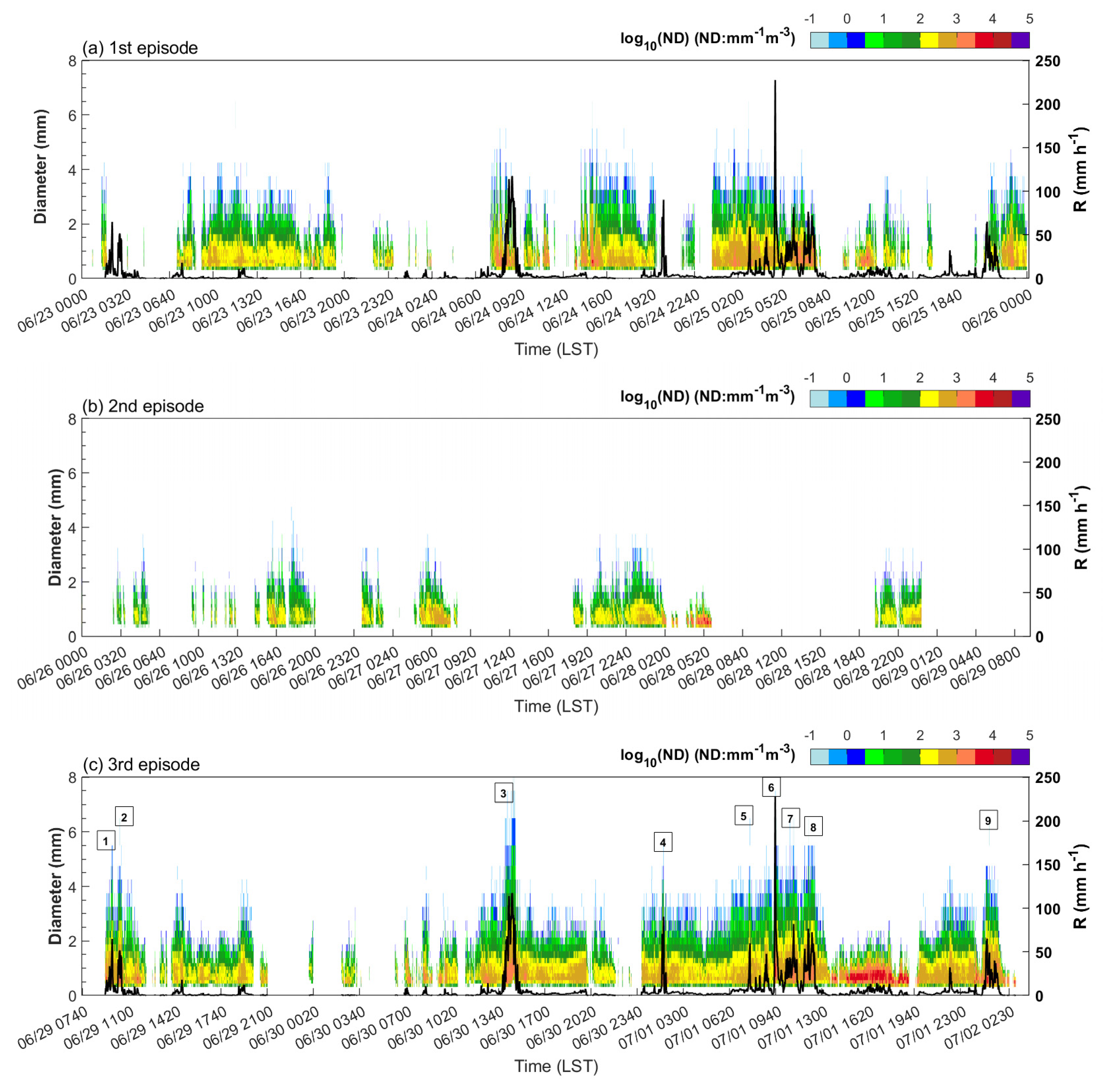
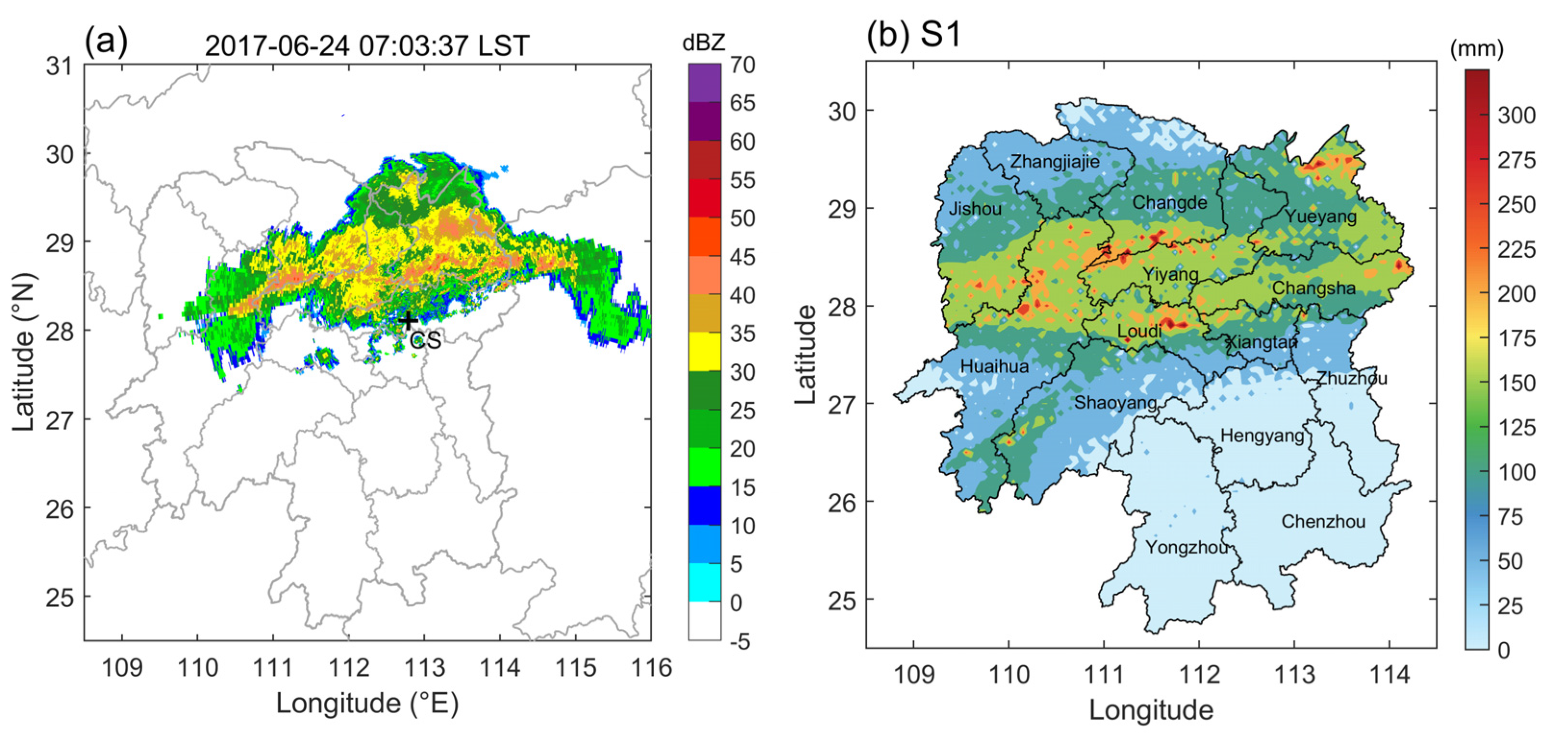
Figure 7 shows the time evolution of DSD and rain rate during the three rainfall episodes observed from the Parsivel² disdrometer at CS sites. Following a brief episode of light rain around 01:40 a.m. LST on 23 June, a period of persistent rain was observed over 12 h starting at 07:13 LST on 23 June (Figure 7a). During the first episode, a few large raindrops with diameters exceeding four mm were occasionally observed in the presence of relatively high concentrations of small and midsize drops. The presence of large drops (>5 mm) along with the abundance of small raindrops were noticed at around 2:52 p.m. LST 24 June and 2:46 a.m. LST 25 June (Figure 7a), which was responsible for the heavy rain and high reflectivity (

Table 1. Rainfall characteristics during the three episodes: number of 1-min samples, accumulated rainfall, and integral rain parameters (rain rate R, liquid water content W, mean mass diameter D_m and total concentration of raindrops N_t) derived from the composite raindrop spectra.

Period	Samples (mins)	Total Rainfall (mm)	R (mm h−1)	W (g m−3)	Dm (mm)	Nt (m−3)
1st episode	2367	171.1	4.34	0.23	1.23	395
2nd episode	1390	17.8	0.78	0.05	0.99	209
3rd episode	3023	350.8	6.98	0.35	1.22	591

). A large rainfall amount with 171.1 mm was recorded by Parsivel² in the first episode (Table 1). Rainfall was then quite sporadic between 10:00 a.m. and 4:50 p.m. LST 25 June, with high concentrations of small drops, with the maximum drop diameter not exceeding 2.8 mm before 12:35 p.m. LST on 25 June, and low concentrations of raindrops were observed until 4:50 p.m. LST 25 June. Finally, high concentrations of small and midsize drops were present due to the passage of the rainband, and the storm ended with a moderate shower.

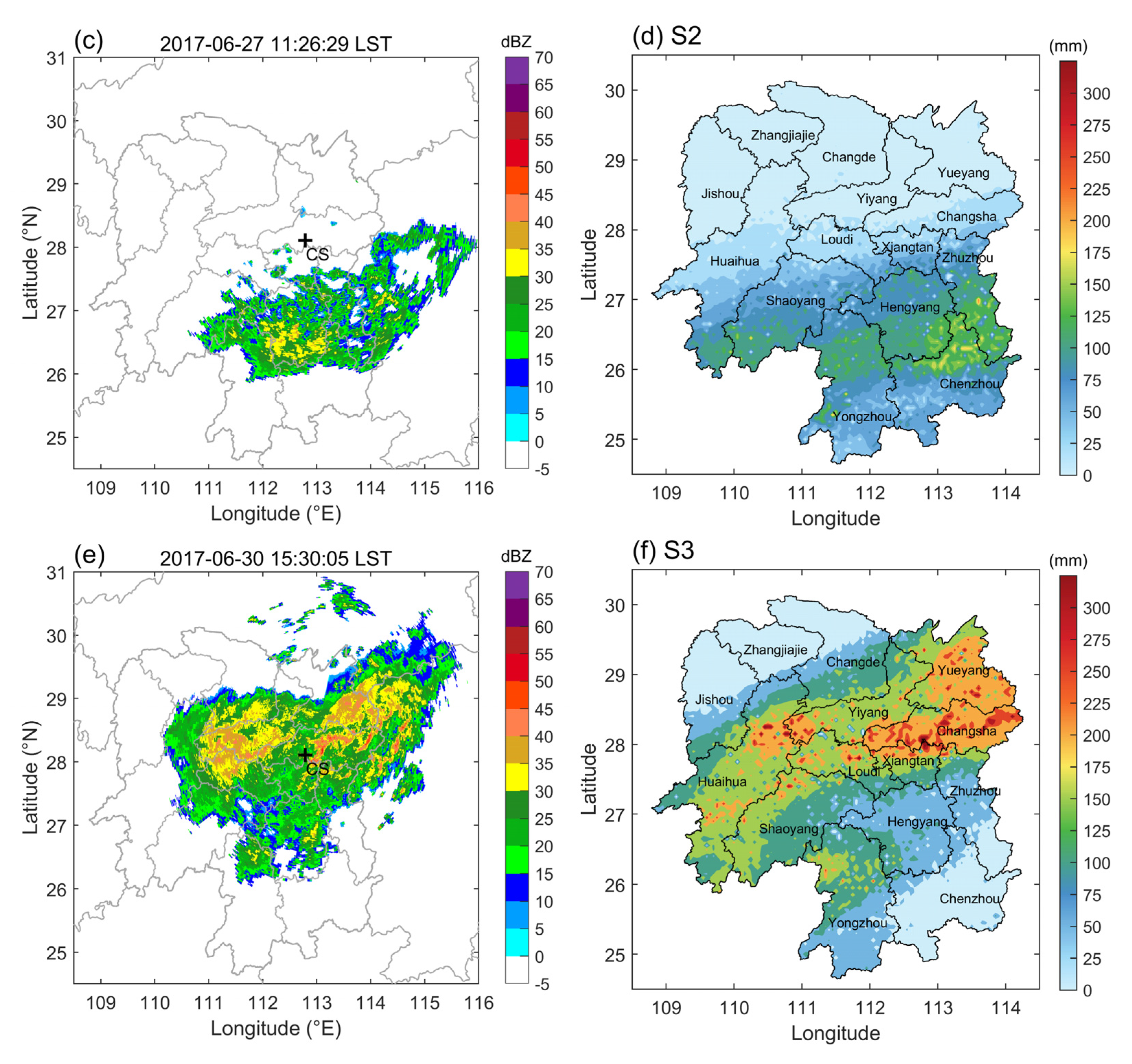
During the second rainfall episode (Figure 7b), rainfall was quite sporadic, and the rain rate was lower than 5 mm h⁻¹ for this whole period with the maximum drop diameter not exceeding 4.8 mm. Low concentrations of small drops were observed throughout the entire episode except for the period between 3:40 a.m. and 6:04 a.m. LST on 28 June when a high concentration of small raindrops dominated. The absence of large raindrops and narrow raindrop spectra results in the lowest D_m, R, W and N_t mean values of 1.07 mm, 0.78 mm h⁻¹, 0.05 g m⁻³ and 209 m⁻³, respectively (Table 1).

The third rainfall episode was the most intense period of this event, having a total rainfall amount of 350.8 mm (Table 1). The time series of the DSD in S3 was distinctly different than the previous two periods. Several periods (denoted as 1 to 9 in Figure 7c) of high concentrations of medium and large drops (D > 5 mm) were observed and the concentration of small raindrops (D < 1 mm) was as high as 10^3.5 mm⁻¹m⁻³, resulting in significant increases in rainfall rate (R > 50 mm h⁻¹). The highest rain rate, 227.5 mm h⁻¹, was observed at 9:38 a.m. LST 1 July when the concentration of midsize drops of 3~5 mm diameter was relatively high. In addition, the highest concentrations (10^4.5 mm⁻¹m⁻³) of small drops (D < 1.0 mm) were noticed in the narrow raindrop spectra where the maximum drop diameter was 2.7 mm between 1:40 p.m. and 7:20 p.m. LST on 1 July. The integrated rainfall parameters, i.e., R, W and N_t, in the third episode also are at their maximum. Compared with the median values of rainfall parameters of the 2013 Great Colorado Flood, the median R, Z and W of the 2017 Great Hunan Flood are smaller, while the median volume diameter D₀ was slightly larger. In terms of its microphysics, such as Z, W, D₀ and N_w, a larger mean diameter of raindrops (i.e., larger D₀) with a relatively lower concentration of raindrops were observed in this event than in that of the 2013 Great Colorado Flood, resulting in higher mean reflectivity and water content in the 2017 Great Hunan Flood.

4.1.2. Composite Raindrop Spectra

Figure 8 shows the composite raindrop spectra for the three different rainfall episodes to further investigate the variations in DSDs, and the gamma distribution parameters derived from the composite DSDs using the truncated moment method are also provided in

Table 2. Gamma distribution parameters (N₀ is the intercept parameter; μ and Λ are the shape and slope parameters, respectively) derived from the composite raindrop spectra during three rainfall episodes using the truncated moment method.

Period	N0 (mm−1-μm−3)	μ	Λ (mm−1)
1st episode	58,264	2.53	5.00
2nd episode	677,035	4.17	8.36
3rd episode	18,877	1.08	3.67

. The maximum concentration occurred at a diameter of 0.56 mm followed by a slow decrease in concentration from the peak to 0.9 mm for the three composite DSDs.

Figure 8 shows the composite DSDs during the three rainfall episodes, revealing the general characteristics of concentration and size distribution of raindrops for the three different rainfall episodes. The numerical concentrations of the small raindrops below 0.5 mm are almost the same, and the difference is obvious from 0.5 mm. The concentration of raindrops for all diameters in the two heavy rainfall periods is higher than that in the second rainfall period with stratiform, indicating that collision-coalescence process is more active during the intense rainfall episodes. Previous studies [24,25,26] with basically different measuring systems and model calculations showed that raindrop spectra have at least one peak, and the first peak usually appeared at the lower end of the measuring scope. According to the diameter classification setting of Parsivel, three raindrop spectra obtained from the Parsivel measurements showed that the highest number of raindrops were between 0.5 and 0.625 mm. The three spectra exponentially decrease with the increasing drop sizes, and the differences of the three DSDs started to be evident from the diameter of 0.5 mm. The concentration of raindrops larger than 0.5 mm was the least during the second episode, resulting in low rainfall intensity and rainwater content (showed in Table 1). The concentrations of small drops with diameter less than 2.0 mm for the first and third intense rainfall episodes were similar, whereas larger concentrations of medium- and large-sized drops (D > 3.0 mm) were observed during S3 where the composite DSD was the widest and the maximum drop diameter was approximately 7.6 mm. Such a DSD of the third episode generated the highest integral rainfall parameters (Table 1). Note that three parameters of the gamma DSD have the lowest values for the third rainfall episode (Table 2).

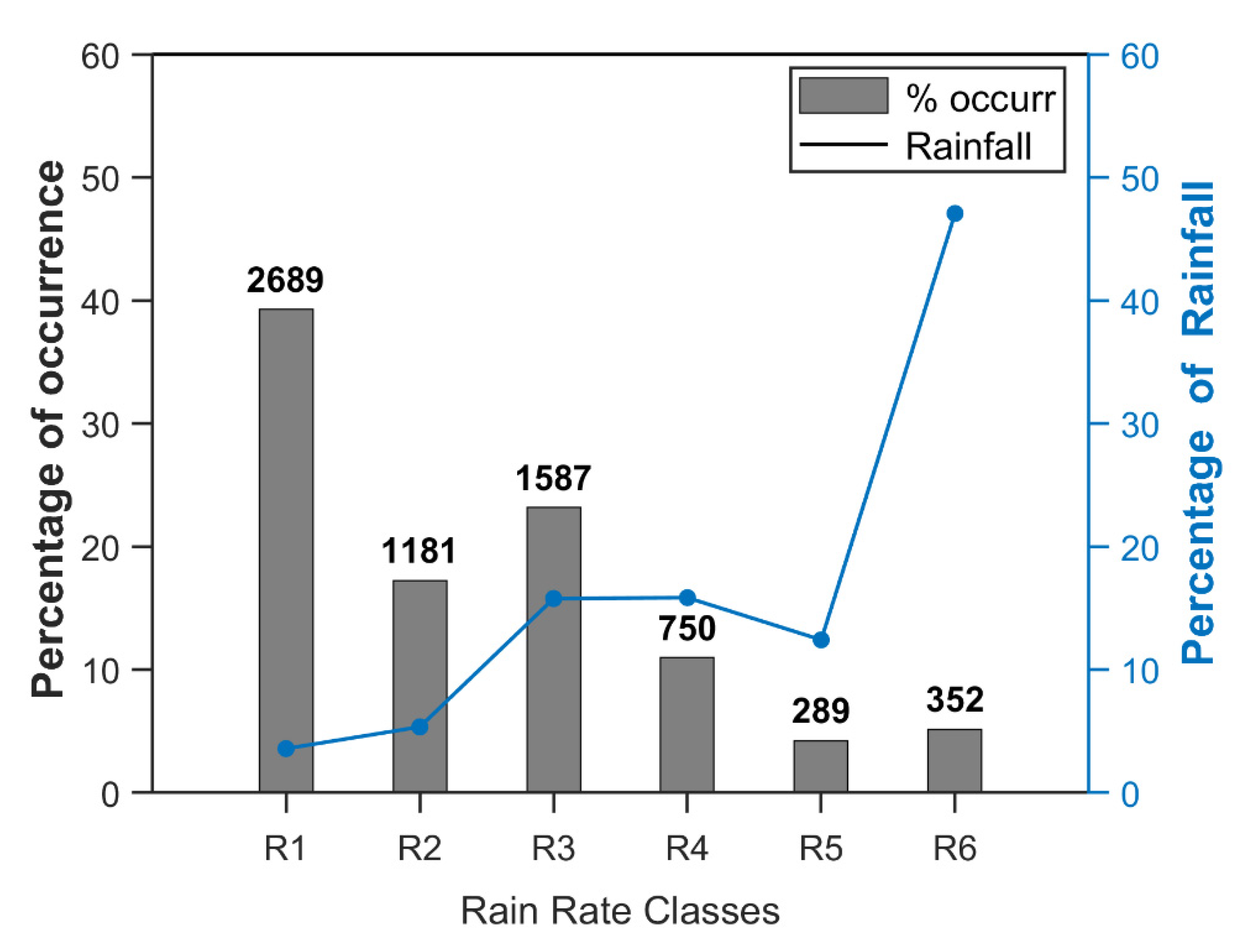
4.1.3. DSD and Rainfall Characteristics for Different Rain Rates

Rainfall microphysical properties vary largely under different rain rates [23,27]. To further investigate the DSD characteristics in different rain rates, the total dataset was divided into six rain rate classes (R1: 0.1 ≤ R < 1, R2: 1 ≤ R < 2, R3: 2 ≤ R < 5, R4: 5 ≤ R < 10, R5: 10 ≤ R < 20, and R6: ≥20 mm h⁻¹) [28]. As shown in Figure 9, the distribution in the percentage of occurrence of R bins is similar to that of the summer rainfall of North Taiwan (Table 4 in Seela et al. [29]), with the highest frequency of occurrence in R1 (39.3%), followed by R3 (23.2%) and R2 (17.2%). The percentage of occurrence of R from small to large is 10.9% in R4, 4.2% in R5 and 5.1% in R6. Even though the occurrence numbers from R1 to R3 vary, a steady increase is observed in the percentage of rainfall relative contribution. R4 contributes to the total rainfall as much as R3, both registering approximately 15.8% of the total rainfall, while the frequency number of R4 was only about half of R3. More than 45% of the total rainfall was from R6, despite its relatively low percentage of occurrence. Although the percentage of occurrence in the R5 category is the lowest, its contribution to the total rainfall is also higher than that of R1 and R2. During the whole rainfall period, more than 55% of total rainfall is contributed by R5 and R6, and these high rain rates lead to the floods and flash floods over the study area because the high probability of occurrences of these rain types is instrumental in causing mountain torrents and debris flows [30,31].

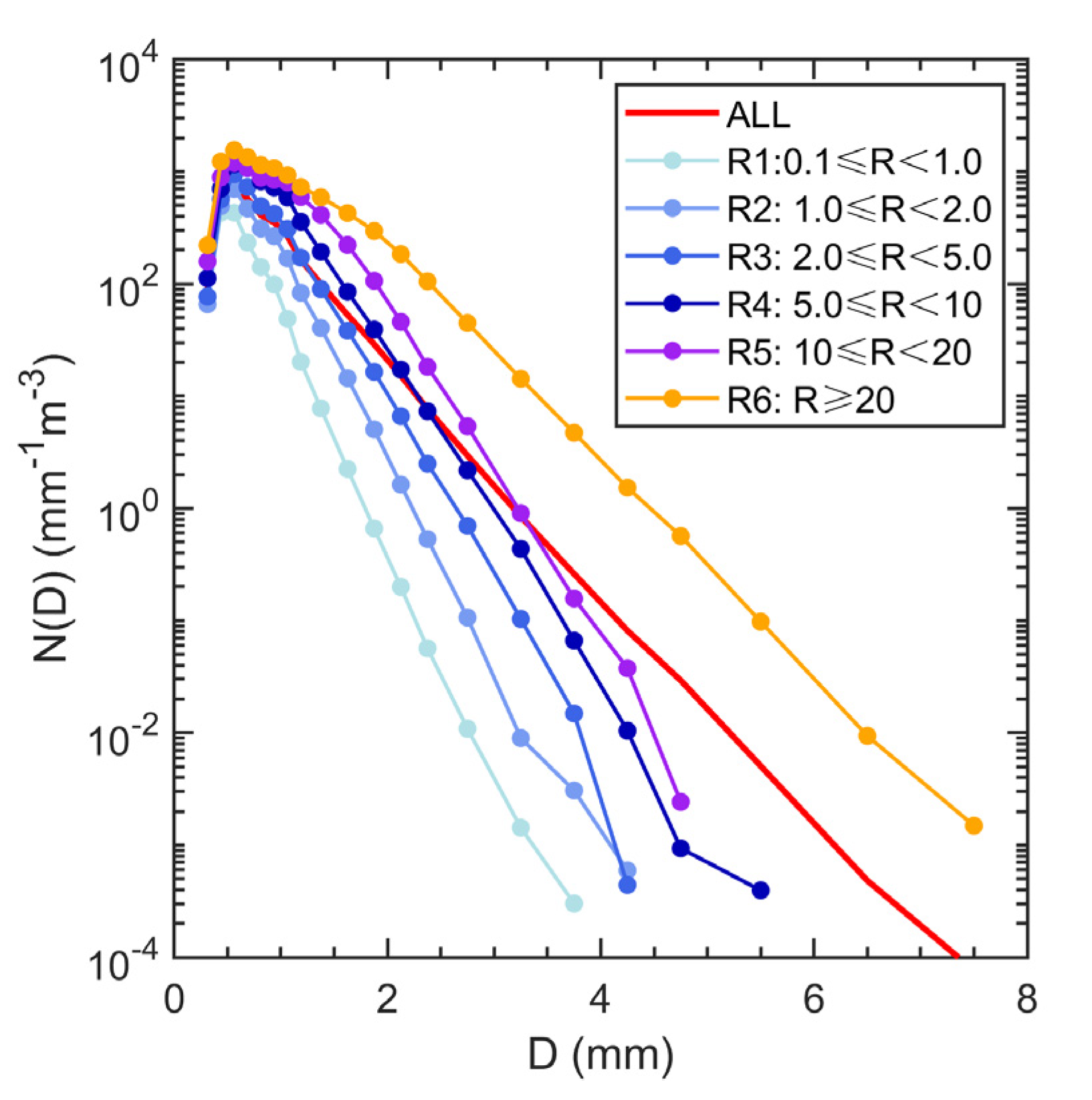
The averaged DSDs in six rain-rate classes were superimposed on the same graph to investigate and compare the characteristics of DSD in different rain rates in Figure 10. Also, the corresponding integral rainfall parameters derived from the average DSD in each rain rate class are presented in

Table 3. Integral rainfall physical quantities (total concentration of raindrops N_t, radar reflectivity Z, liquid water content W, median-volume diameter D₀, mass-weighted mean diameter D_m, and normalized intercept parameter (log₁₀N_w)) derived from the averaged DSDs and the fitted gamma distribution parameters (intercept parameter (log₁₀N₀), shape μ and slope parameter Λ) in different rain rate classes.

Class	Nt (m−3)	Z (dBZ)	W (g m−3)	D0 (mm)	Dm (mm)	log10Nw	log10N0	μ	Λ (mm−1)
Total	452.20	35.66	0.25	1.33	1.61	3.48	5.52	0.28	2.62
R1 (0.1~1.0)	187.81	18.80	0.03	0.80	0.91	3.60	5.50	3.70	8.44
R2 (1.0~2.0)	335.93	25.88	0.10	0.97	1.10	3.73	5.15	3.27	6.58
R3 (2.0~5.0)	504.13	30.75	0.20	1.09	1.26	3.81	4.77	2.55	5.21
R4 (5.0~10.0)	781.81	34.88	0.39	1.14	1.37	3.96	4.84	2.59	4.80
R5 (10~20)	1012.42	38.61	0.73	1.34	1.53	4.04	5.04	3.46	4.88
R6 (>20)	1465.62	47.15	1.91	1.83	2.07	3.93	4.23	1.83	2.81

, and the values associated with the entire datasets are also given in Table 3 and Figure 10. The spectral width of DSDs increases with the rain rate and the shape of DSD becomes flatter due to the contribution of large raindrops (Figure 10) which led to larger integral rainfall properties, such as N_t, Z, W, and D_m (Table 3), in higher rainfall rates. The gamma parameters, N₀, μ and Λ, decrease with an increased rain rate from R1 to R4. Note that the maximum N_w appeared in R5 and there is an increase for each gamma parameter at R5. This may be related to the apparent variation of DSD shape at R5 (Figure 10) where a bi-modal shape with the peaks at 0.56 and 1.06 mm occurred. The minimum values of N₀, μ and Λ are found in R6, corresponding to the widening and flattening of the DSD shape. For the entire rainfall period, the shape of DSD is close to an exponential distribution with shape parameter μ of 0.28. Compared with the composite raindrop spectrum in the same rain rate class of the 2016 ”7.20” Beijing rainstorm [32], the DSDs under the R1-R3 classes show high similarities in the two events. In R4 and R5, the number densities of drops with diameters smaller than 0.5 mm and larger than 2.0 mm of the 2017 Great Hunan Flood are lower than that of the 2016 ”7.20” Beijing rainstorm, while the number of raindrops in the middle size is higher in the former event. In the highest rain rate R6 class, medium- to large-sized drops (D > 2 mm) with larger concentrations were observed in the 2017 Great Hunan Flood despite that the number density of tiny raindrops (D < 0.8 mm) of the 2016 “7.20” Beijing rainstorm is higher up to 1–2 orders of magnitude. Therefore, higher values of W, Z and D_m are observed in the 2017 Great Hunan Flood.

4.1.4. Distribution of D_m and N_w

Many studies have thoroughly detailed the different characteristics of DSD in convective and stratiform rain, and they are related to the cloud microphysical processes and vertical motions for each rain type [28,33,34,35,36,37]. Additionally, the distribution of D_m and log₁₀N_w are often used to characterize the convective precipitation as being continental or maritime (e.g., [34,38,39]). Figure 11 shows the frequency distributions of D_m versus log₁₀N_w during the three episodes. The D_m-log₁₀N_w pairs mainly reside on both sides of the stratiform line according to Bringi et al. [31], with the mean value of D_m near 1.2 mm and log₁₀N_w of 3.65 (the 1st episode) and 3.83 (the 2nd episode) (Figure 11a, c). During the second episode, a larger proportion of data (>15%) exists near log₁₀N_w = 3.4 and D_m = 1.0 mm, corresponding to stratiform rain in Bringi et al. [34] (Figure 11b). It is worth noting that some scatter during S2 and S3 have high values of log₁₀N_w (>4.5) but low D_m (<1.0 mm), which appear at 4:10~6:00 a.m. LST on 28 June 2017 (during S2) and 11:45 a.m. ~8:00 p.m. LST on 1 July 2017 (during S3), where intense convective rainfall passed over the site with radar reflectivity higher than 50 dBZ, with the maximum drop diameter on the ground small to 2.5 mm (Figure 7b, c). This may be related to the shallow convective rain characterized by a relatively small maximum diameter and high concentration of raindrops with small diameters, as recorded in Wen et al. [39]. 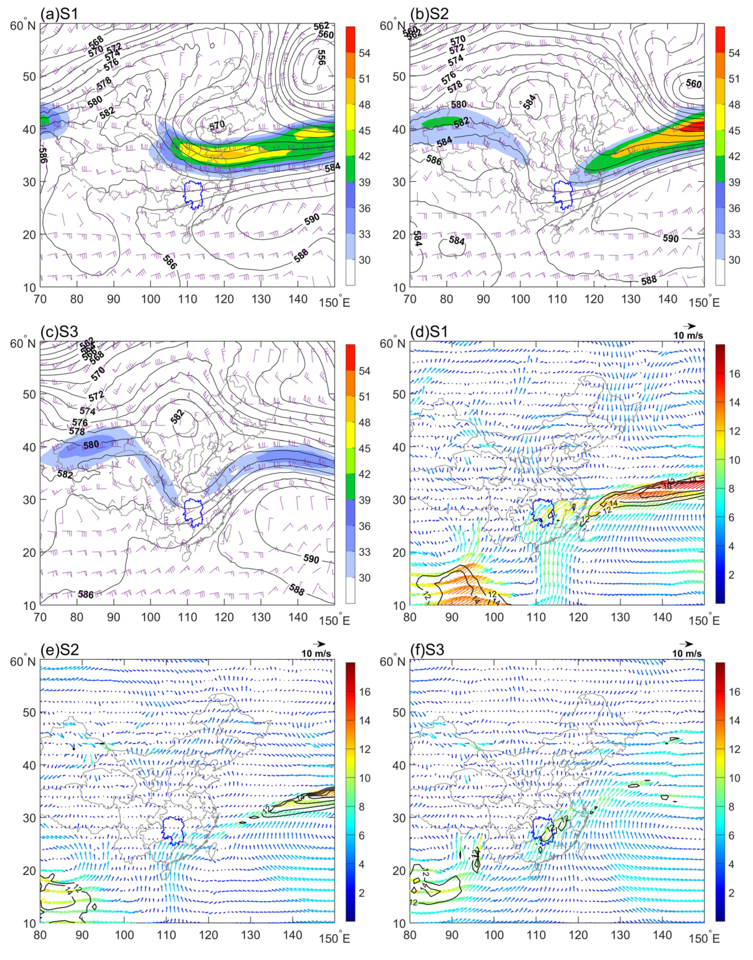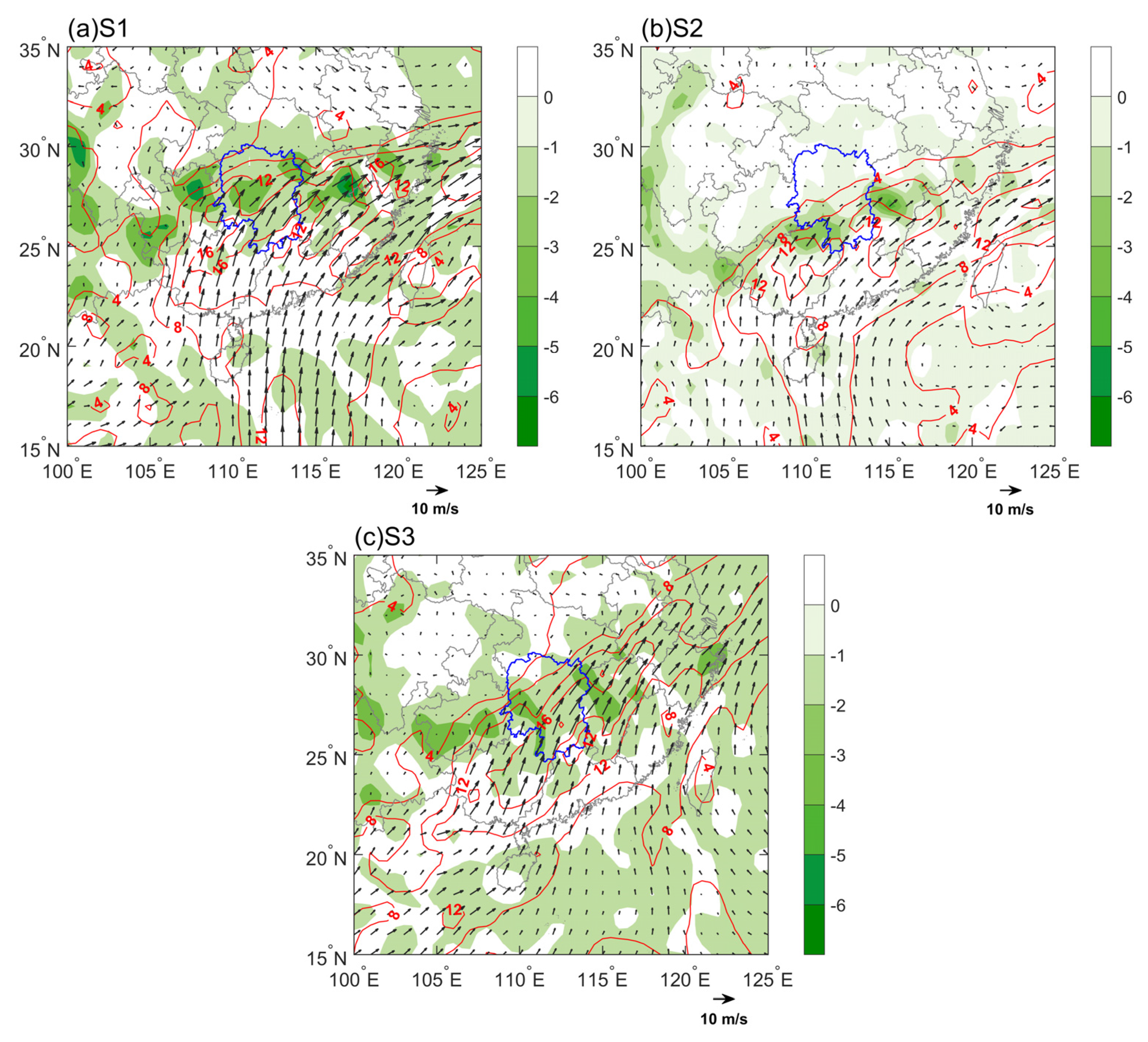Besides, some scatter distributed on the right side of the stratiform line are closer to the maritime convection cluster (Figure 11a), although the CS site is located in the inland, and this feature is more evident during the third episode (Figure 11c), indicating that the convective rainfall during the 2017 Great Hunan Flood is characterized by a high concentration of small raindrops. On the one hand, this flood occurred between late June and early July during the Mei-yu (called Baiu in Japan) period, and the adequate vapor during the Asian summer monsoon season from the Bay of Bengal and the South China Sea (Figure 6) might limit the evaporation processes of raindrops. On the other hand, the mean CAPE values calculated from in- situ sounding data at the CS site are high at 275.9 J kg⁻¹ and 1006.2 J kg⁻¹ during S1 and S2, respectively, suggesting relatively intense convective activities during both periods. The stronger convective activity contributes to the collision-breakup processes in heavy rain; as a result, there are abundant small raindrops.

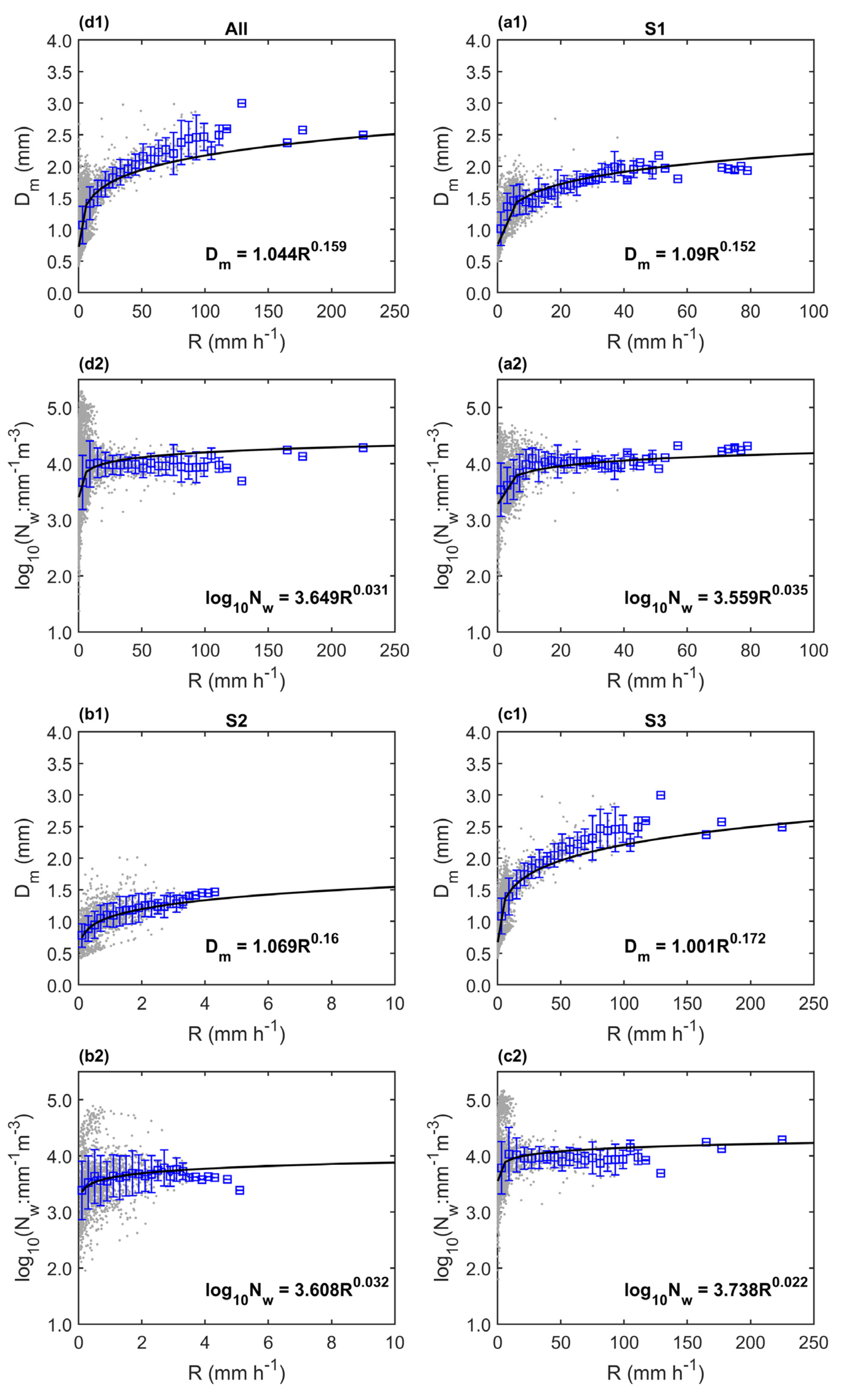
Figure 12 presents the D_m and log₁₀N_w vary with R to further investigate the variability of the two parameters with respect to rain rates, and the fitted power-law relationships using a least-squares method are also provided. The variability of D_m and log₁₀N_w with the rain rate shows similarity in the three episodes. The standard deviations of both parameters decrease with the rain rate. The D_m increases with the rain rate, and the indexes of D_m-R relationships are greater than 0.15. The indexes of log₁₀N_w-R relationships are close to 0, and the log₁₀N_w converges with the increasing rain rate. This suggests that the concentration of raindrops remains constant at a high rain intensity, while any increase in rain rate is mainly due to an increase in the size of raindrops, which is contrary to the situations in Nanjing, eastern China [39] and Zhuhai, southern China [40], where the increase in rain rate is mainly due to the increase of raindrop concentration. These results reveal the unusualness of the DSD for the 2017 Great Hunan Flood. At high rain rates, the DSDs may reach a size-controlled state where raindrops are neither created (no coalescence) nor destroyed (no breakup), that is, the drop concentration remains approximately constant and grows by accretion of cloud droplets [41].

It is possible to establish an empirical relationship between N_w and D_m since the two parameters are related and not independent [38], and this relation was normally used in the GPM DPR rainfall retrieval [42]. Figure 13 shows the N_w-D_m distribution under different rain rates, and one can see that there is a good correlation between N_w and D_m within a specific range of rainfall rates.

Table 4. Coefficients of the fitted relations between log₁₀N_w (N_w: mm⁻¹m⁻³) and D_m (mm) and coefficients of determination (R²) for the second-degree polynomial equations in six rain rate categories (R1~R6) and the total data set.

Class	log10Nw = aDm2 + bDm + c
	a	b	c	R2
R1 (0.1~1.0)	0.6395	−3.1403	5.8829	0.7642
R2 (1.0~2.0)	0.8244	−3.7124	6.8186	0.9543
R3 (2.0~5.0)	0.9785	−4.0699	7.3432	0.9285
R4 (5.0~10.0)	0.5398	−3.0356	7.0993	0.9657
R5 (10~20)	0.3465	2.3050	6.7054	0.9185
R6 (>20)	0.0165	0.4715	4.8474	0.4175
All	0.6411	−2.0426	5.1380	0.1749

summarized the statistical results for each N_w-D_m relation in different rain rate classes. The coefficients of determination R² were high (>0.91) from the R2 to R5 classes, but they are lower in light rain (R < 1.0 mm h⁻¹) and intense rain (R > 20 mm h⁻¹). This is consistent with the variation of log₁₀N_w and D_m with rain rates as shown in Figure 12. The distributions of D_m and log₁₀N_w are scattered in low rain rates with relatively higher standard deviations, resulting in a low value of R² (0.76) in the regression between D_m and log₁₀N_w. The second-degree polynomial equation fitted the data least well in the highest rain rate class with R² of ~0.42 due to the increase of D_m and approximate invariability of log₁₀N_w in the high range of R (>20 mm h⁻¹). For the whole data set of this event, the coefficients of determination R² are only 0.2, indicating that the polynomial equation can hardly represent the log₁₀N_w-D_m relationship very well. Therefore, using GPM DPR observations to derive the parameters N_w and D_m in different rainfall rate classes by applying the corresponding log₁₀N_w-D_m relationships may help to improve the accuracy of rainfall retrieval from GPM DPR measurements.

4.2. QPE

Radar quantitative precipitation estimation (QPE) is one of the applications of DSDs. The analyses above show that DSDs, rainfall parameters, and the gamma function parameters differ among the first, second and third episodes, and one may wonder how that affects the radar reflectivity-rain rate (Z-R) relationship. Previous studies have shown that the coefficient (A) and exponent (b) of radar reflectivity-rain rate (Z = AR^b) relations strongly depend on DSD variability [7]. Figure 14a shows the Z-R relationships for the entire event and the three rainfall episodes derived from the 1-min DSD samples. For comparison, Z = 300R^1.4 for the standard NEXRAD Z-R relationship used in the China and United States is also provided. For this rainfall event, the exponents of the Z-R relationship are around 1.4, while the disparities are obvious in coefficients of A. When the rain rate is smaller than 10 mm h⁻¹, the power-law Z = 175.681R^1.426 derived from the third rainfall episode observations gives the highest rain rate estimation for a given radar reflectivity. All the Z-R relationships obtained in this rainfall event lie under the standard NEXRAD Z-R relation, indicating that using the standard Z-R relationship with A = 300 and b = 1.4 in the weather radar would give an underestimation for this rainstorm.

We used the rain gauges deployed within radar coverage to evaluate the performance of the NEXRAD Z-R relationship-based quantitative precipitation estimation from the S-band weather radar for the 2017 Great Hunan Flood. In this paper, the data from 0.5° elevation angle PPI (plan position indicator) in the range between 15 and 120 km of radar are used to estimate surface rainfall, and the 1-h rainfall accumulation was used for comparison with rain gauge data. The CC, RMSE, and NE of the NEXRAD Z-R relationship are 0.89, 3.80 mm, and 0.36, respectively (Figure 14b). In terms of relative bias, the Z-R relationship commonly used by operational NEXRAD strongly underestimated hourly rainfall by up to 27.5%, indicating that the single-polarization radar variable was too weak to be useful for rain-rate estimations.

4.3. Rainfall Erosivity Estimation

There have been diverse KE_mm-R relationships developed due to the more widespread use of KE_mm [20], such as logarithmic [43], polynomial [44], exponential [22,45], linear [46], or power law [47]. Therein, the most used are the logarithmic and exponential forms. According to Salles et al. [21], KE_time provides a better correlation between KE and R than KE_mm, and power-law and linear function are common in the regression of KE_time-R. Figure 15 presents the scatterplots of KE_time and KE_mm versus R for the three rainfall episodes of the 2017 Great Hunan Flood. Here, the linear, polynomial and power-law equations are used in KE_time-R fitting, and the power, exponential and logarithmic equations are applied in KE_mm-R regression. As Figure 15 shown, KE_time increases more linearly with rain rate R than KE_mm. At relatively lower R values, for each rainfall episode, the three fitting lines of KE_time -R are almost overlapping while deviating more and more obviously with the increase of rain rate, especially the linear fitting curves that give the lowest KE estimations under the same rainfall intensity than the other two models (Figure 15a–c). From the statistical results for each rainfall episode in

Table 5. Coefficients of determination (R²), root mean squared error (RMSE) and, normalized absolute error (NE) for KE_time-R equations applied to three different rainfall episodes.

Rainfall Episodes	Statistics	KEtime-R
		Linear	Polynomial	Power Law
1st episode		KEtime = 16.21R − 14.53	KEtime = 0.08R2 + 12.90R − 6.05	KEtime = 8.15R1.19
	R2	0.9608	0.9732	0.9761
	RMSE	24.3181	20.1161	18.9612
	NE	0.2632	0.1807	0.161
2nd episode		KEtime = 10.58R − 1.68	KEtime = 1.49R2 + 6.43R − 0.26	KEtime = 7.63R1.32
	R2	0.8790	0.9032	0.9001
	RMSE	2.7952	2.4999	2.5389
	NE	0.2722	0.2158	0.2187
3rd episode		KEtime = 20.3R − 33.75	KEtime = 0.01R2 + 19.17R − 29.34	KEtime = 10.73R1.14
	R2	0.9501	0.9512	0.9546
	RMSE	69.733	68.9328	66.5323
	NE	0.3059	0.2781	0.1962

, one can see that the regression between KE_time and R with power-law and polynomial equations are similar and better than the linear function. Moreover, three equations perform better during the intense rainfall episodes and produced a higher coefficient of determination and less dispersion.

Figure 15d–f show that the relationship between KE_mm and R is nonlinear and KE_mm present a high dispersion of values compared to KE_time. Specifically, for the second rainfall episode dominated by the light rain intensity, the KE_time-R pairs do not show a clear structure and all the three equations show poor performances in the regressions among the three rainfall episodes (

Table 6. As in Table 5, but for KE_mm-R relationships.

Rainfall Episodes	Statistics	KEmm-R
		Exponential	Logarithmic	Power Law
1st episode		KEmm = 25.92 (1 − 0.72e−0.03R)	KEmm = 8.27 + 4.45log10R	KEmm = 8.01R0.2
	R2	0.3491	0.5058	0.4995
	RMSE	3.1784	2.7695	2.7881
	NE	0.2768	0.2300	0.2340
2nd episode		KEmm = 21.81 (1 − 0.79e−0.18R)	KEmm = 7.91 + 3.97log10R	KEmm = 7.84R0.28
	R2	0.3446	0.3612	0.3741
	RMSE	2.3950	2.3646	2.3405
	NE	0.2780	0.2690	0.2680
3rd episode		KEmm = 31.91 (1 − 0.79e−0.02R)	KEmm = 7.11 + 5.26log10R	KEmm = 6.8R0.25
	R2	0.5438	0.5854	0.6293
	RMSE	3.0046	2.8555	2.7000
	NE	0.2578	0.2359	0.2230

). The power-law equation shows the best fit in the third intense rainfall episode with the highest coefficients of determination R² of 0.63 and relatively low RMSE (2.77) and NE (0.22) values, whereas the logarithmic equation is fitting best for the first rainfall episode and the statistical parameters are close to that from the power-law regression. Overall, compared with KE_time-R relationships, there is not a clear relationship between KE_mm-R. Therefore, KE_time-R relationships are preferable for erosivity estimation of each rainfall episode for this event.

According to Torres et al. [46], the kinetic energy can be expressed by the median-volume drop diameter D₀ using the D₀ (R) relations. Wen et al. [48] proposed a polynomial relation between KE_mm and D_m: KE_mm = −2.33 D_m ²+21.05D_m − 7.79, with the coefficient of determination R² of 0.94 and RMSE of 1.41 J m⁻² mm⁻¹ using data from Nanjing, eastern China. Figure 16 depicts the relations between KE_mm and D_m. From Figure 16, the differences among the three fitting cures for the same rainfall period are very small, and the distinction is only notable in the larger D_m end. In addition, the fitting performance of the same equation to the KE_mm-D_m is better than that of KE_time-R according to the statistical results in

Table 7. As in Table 5, but for KE_mm-D_m relationships.

Rainfall Episodes	Statistics	KEmm-Dm
		Linear	Polynomial	Power Law
1st episode		KEmm = 11.35Dm − 4.69	KEmm = 0.51Dm2 + 10.07Dm − 3.94	KEmm = 6.63Dm1.50
	R2	0.9647	0.9651	0.9608
	RMSE	0.7402	0.7361	0.7837
	NE	0.0571	0.0568	0.0616
2nd episode		KEmm = 11.43Dm − 4.62	KEmm = 0.82Dm2 + 9.77Dm − 3.82	KEmm = 6.60Dm1.65
	R2	0.9565	0.9573	0.9473
	RMSE	0.6168	0.6116	0.6793
	NE	0.0656	0.0656	0.0780
3rd episode		KEmm = 10.88Dm − 4.25	KEmm = −0.15Dm2 + 11.27Dm − 4.94	KEmm = 6.68Dm1.40
	R2	0.9599	0.9599	0.9499
	RMSE	0.8885	0.8878	0.9929
	NE	0.0642	0.0644	0.0744

. Amazingly, the coefficients of determination R² are ≥0.95, RMSE and NE values have no significant differences in rainfall episodes and different equations, implying a good performance for rainfall KE_mm estimation using the KE_mm-D_m estimator.

5. Summary and Conclusions

During the 2017 Great Hunan Flood from 22 June to 2 July 2017, detailed data from a Parsivel disdrometer, a ground-based dual S-band Doppler weather radar, located at Changsha site, Hunan province, southern China, and 357 rain gauges scattered in the province, were used to measure the microphysical characteristics of this persistent rainfall. Due to its long duration, the spatial and temporal variations of DSD, rainfall parameters (R, Z, D₀, and W), and derived relationships (i.e., radar reflectivity-rain rate and rainfall kinetic relations) were derived and compared in three different rainfall episodes.

This rainfall event lasted for a long time and affected a wide range, with the maximum total rainfall observed by Parsivel² of 543 mm at the Changsha site. Rainfall throughout the entire event was characterized by a large number of small- to medium-sized raindrops (diameter D < 1.5 mm), resulting in the highest concurrency frequency of the small rain rate category (0.1 < R < 1.0 mm h⁻¹). The spatial distribution characteristics of rainfall are different in three episodes, and each episode presents a different DSD feature.

The first rainfall episode was mainly composed of a small concentration of raindrops, and the N (D) of the second episode was the lowest. During the third rainfall episode, the highest concentration of small droplets (D < 1 mm) and large raindrops (D > 4 mm) was observed, resulting in the largest integral rainfall parameters and rainfall kinetic energy (KE). The patterns of the variation of D_m and log₁₀N_w with rainfall intensity were quite similar among the three episodes: D_m increases with the rain rate while the log₁₀N_w converges with the increasing rain rate. In addition, the D_m versus log₁₀N_w pairs of the first and third intense rainfall episodes are plotted roughly around the “maritime” cluster, indicating a maritime nature of convective precipitation throughout the flood.

The DSD-derived Z-R relations from the disdrometer reflect how unusual the DSD was during the 2017 Great Hunan Flood. A larger concentration of medium- to large-sized drops (D > 3 mm) was observed during the third intense rainfall episode, accompanied by an increase in liquid water content, medium volume diameter and reflectivity. As a result, the Z-R relationship (Z = AR^b) showed the smallest coefficient (A = 175.15) and largest exponent (b = 1.43) compared to raindrop spectra during the first and second rainfall episodes. Nevertheless, these values were smaller than the values of the ‘‘standard’’ NEXRAD Z-R relationship (Z = 300R^1.4), leading to an underestimation of radar-based hourly rainfall by 27.5%.

A critical comparison of different formulae relating rainfall intensity (R) and kinetic energy (KE), as well as mean mass-weighted diameter (D_m) and KE, was performed using direct DSD measurements of this flood during the three rainfall episodes. Nine functions to predict two types of KE (KE_time and KE_mm) from R and D_m, were obtained. The fitting effects of the same function for the first and third intense rainfall episodes were better than that for the second rainfall episode. When KE is related to R, the KE_time expression was preferred over KE_mm, and a power-law function showed the best regression between KE_time and R. On the other hand, the comparison between KE_mm-D_m and KE_mm-R concludes that D_m is more appropriate to be linked to KE_mm than R and KE_time-R relationships for erosivity estimation.

References

1. Tang, Y.; Gan, J.; Zhao, L.; Gao, K. On the climatology of persistent heavy rainfall events in China. Adv. Atmos. Sci. 2006, 23, 678–692. [Google Scholar] [CrossRef]
2. Friedrich, K.; Kalina, E.A.; Aikins, J.; Steiner, M.; Gochis, D.; Kucera, P.A.; Ikeda, K.; Sun, J.Z. Raindrop size distribution and rain characteristics during the 2013 great Colorado flood. J. Hydrometeorol. 2016, 17, 53–72. [Google Scholar] [CrossRef]
3. Jin, L.; Huang, C.; Zhu, C.; Liu, J.; Zhang, L.; Gao, W. Diagnostic Analysis of Flood-resulting Rainstorm over Hunan Province in June 2017. J. China Hydrol. 2018, 38, 91–96. (In Chinese) [Google Scholar]
4. Chen, H.; Ye, C.; Chen, J.; Luo, Z. Analysis of Water Vapor Transport and Budget During Persistent Heavy Rainfall over Hunan Province in June 2017. Meteorol. Mon. 2019, 45, 1213–1226. (In Chinese) [Google Scholar] [CrossRef]
5. Li, Y.; Luo, B.; Peng, L.; Zhang, C. Diagnostic analysis of dynamical parameters for Hunan persistent heavy rain event in late June 2017. Torrential Rain Disasters 2020, 39, 10–19. (In Chinese) [Google Scholar] [CrossRef]
6. Boucher, O.; Randall, D.; Artaxo, P.; Bretherton, C.; Feingold, G.; Forster, P.; Kerminen, V.M.; Kondo, Y.; Liao, H.; Lohmann, U.; et al. Clouds and aerosols. In Climate Change 2013: The Physical Science Basis. Contribution of Working Group I to the Fifth Assessment Report of the Intergovernmental Panel on Climate Change; Stocker, T.F., Qin, D., Plattner, G.-K., Tignor, M., Allen, S.K., Doschung, J., Nauels, A., Xia, Y., Bex, V., Midgley, P.M., Eds.; Cambridge University Press: Cambridge, UK, 2013; pp. 571–657. [Google Scholar] [CrossRef]
7. Rosenfeld, D.; Ulbrich, C.W. Cloud Microphysical Properties, Processes, and Rainfall Estimation Opportunities. Meteorol. Monogr. 2003, 52, 237–258. [Google Scholar] [CrossRef]
8. Bringi, V.N.; Chandrasekar, V. Polarimetric Doppler Weather Radar: Principles and Applications; Cambridge University Press: Cambridge, UK, 2001. [Google Scholar] [CrossRef]
9. Caracciolo, C.; Napoli, M.; Porcu, F.; Prodi, F.; Dietrich, S.; Zanchi, C.; Orlandini, S. Raindrop Size Distribution and Soil Erosion. J. Irrig. Drain. Eng. 2012, 138, 461–469. [Google Scholar] [CrossRef]
10. Liao, L.; Meneghini, R. A study of air/space-borne dual-wavelength radar for estimation of rain profiles. Adv. Atmos. Sci. 2005, 22, 841–851. [Google Scholar] [CrossRef]
11. Testik, F.Y.; Barros, A.P. Toward elucidating the microstructure of warm rainfall: A Survey. Reviews of Geophysics. 2007, 45, 1–21. [Google Scholar] [CrossRef]
12. Testud, J.; Oury, S.; Black, R.A.; Amayenc, P.; Dou, X.K. The concept of “normalized’’ distribution to describe raindrop spectra: A tool for cloud physics and cloud remote sensing. J. Appl. Meteorol. 2001, 40, 1118–1140. [Google Scholar] [CrossRef]
13. Löffler-Mang, M.; Joss, J. An Optical Disdrometer for Measuring Size and Velocity of Hydrometeors. J. Atmos. Ocean. Technol. 2000, 17, 130–139. [Google Scholar] [CrossRef]
14. Jaffrain, J.; Berne, A. Experimental quantification of the sampling uncertainty associated with measurements from PARSIVEL disdrometers. J. Hydrometeorol. 2011, 12, 352–370. [Google Scholar] [CrossRef]
15. Brandes, E.A.; Zhang, G.F.; Vivekanandan, J. Experiments in Rainfall Estimation with a Polarimetric Radar in a Subtropical Environment. J. Appl. Meteorol. 2002, 41, 674–685. [Google Scholar] [CrossRef] [Green Version]
16. Wen, L.; Zhao, K.; Zhang, G.F.; Liu, S.; Chen, G. Impacts of instrument limitations on estimated raindrop size distribution, radar parameters, and model microphysics during mei-yu season in East China. J. Atmos. Ocean. Technol. 2017, 34, 1021–1037. [Google Scholar] [CrossRef]
17. Tokay, A.; Petersen, W.A.; Gatlin, P.; Wingo, M. Comparison of Raindrop Size Distribution Measurements by Collocated Disdrometers. J. Atmos. Ocean. Technol. 2013, 30, 1672–1690. [Google Scholar] [CrossRef]
18. Ulbrich, C.W. Natural variations in the analytical form of the raindrop size distribution. J. Clim. Appl. Meteorol. 1983, 22, 1764–1775. [Google Scholar] [CrossRef] [Green Version]
19. Vivekanandan, J.; Zhang, G.F.; Brandes, E. Polarimetric radar estimators based on a constrained gamma drop size distribution model. J. Appl. Meteorol. 2004, 43, 217–230. [Google Scholar] [CrossRef] [Green Version]
20. van Dijk, A.; Bruijnzeel, L.A.; Rosewell, C.J. Rainfall intensity-kinetic energy relationships: A critical literature appraisal. J. Hydrol. 2002, 261, 1–23. [Google Scholar] [CrossRef]
21. Salles, C.; Poesen, J.; Sempere-Torres, D. Kinetic energy of rain and its functional relationship with intensity. J. Hydrol. 2002, 257, 256–270. [Google Scholar] [CrossRef]
22. Kinnell, P.I.A. Rainfall Intensity-Kinetic Energy Relationships for Soil Loss Prediction. Soil Sci. Soc. Am. J. 1981, 45, 153–155. [Google Scholar] [CrossRef]
23. Chen, B.; Hu, Z.; Liu, L.; Zhang, G. Raindrop Size Distribution Measurements at 4,500m on the Tibetan Plateau during TIPEX-III. J. Geophys. Res. Atmos. 2017, 122, 11092–11106. [Google Scholar] [CrossRef]
24. List, R.; Donaldson, N.R.; Stewart, R.E. Temporal Evolution of Drop Spectra to Collisional Equilibrium in Steady and Pulsating Rain. J. Atmos. Sci. 1987, 44, 362–372. [Google Scholar] [CrossRef] [Green Version]
25. Steiner, M.; Waldvogel, A. Peaks in Raindrop Size Distributions. J. Atmos. Sci. 1987, 44, 3127–3133. [Google Scholar] [CrossRef] [Green Version]
26. Willis, P.T. Functional Fits to Some Observed Drop Size Distributions and Parameterization of Rain. J. Atmos. Sci. 1984, 41, 1648–1661. [Google Scholar] [CrossRef] [Green Version]
27. Nzeukou, A.; Sauvageot, H.; Ochou, A.D.; Kebe, C.M.F. Raindrop Size Distribution and Radar Parameters at Cape Verde. J. Appl. Meteorol. 2004, 43, 90–105. [Google Scholar] [CrossRef]
28. Tokay, A.; Short, D.A. Evidence from tropical raindrop spectra of the origin of rain from stratiform versus convective clouds. J. Appl. Meteorol. 1996, 35, 355–371. [Google Scholar] [CrossRef] [Green Version]
29. Seela, B.K.; Janapati, J.; Lin, P.-L.; Wang, P.K.; Lee, M.-T. Raindrop Size Distribution Characteristics of Summer and Winter Season Rainfall Over North Taiwan. J. Geophys. Res. Atmos. 2018, 123, 11602–11624. [Google Scholar] [CrossRef] [Green Version]
30. Vishnu, R.; Das, S.M.; Sampath, S.; Kumar, G.M. Detection of Possible Thunderstorm Formation Inferred from Weather Element Changes at Ground Level on a Mountain Slope. J. Light. Res. 2010, 2, 12–24. [Google Scholar] [CrossRef] [Green Version]
31. Vishnu, R.; Kumar, A.; Sreekanth, T.S.; Symon, V.N.S.; Das, S.M.; Kumar, G.M. Formation of thunderclouds in a region of high lightning incidence inferred from AWS, Ceilometer and an Electric Field Mill. In Proceedings of the 2011 7th Asia-Pacific International Conference on Lightning, Chengdu, China, 1–4 November 2011. [Google Scholar] [CrossRef]
32. Luo, L.; Xiao, H.; Yang, H.; Chen, H.; Guo, J.; Sun, Y.; Feng, L. Raindrop size distribution and microphysical characteristics of a great rainstorm in 2016 in Beijing, China. Atmos. Res. 2020, 239, 104895. [Google Scholar] [CrossRef]
33. Atlas, D.; Ulbrich, C.W.; Marks, F.D.; Black, R.A.; Amitai, E.; Willis, P.T.; Samsury, C.E. Partitioning tropical oceanic convective and stratiform rains by draft strength. J. Geophys. Res. Atmos. 2000, 105, 2259–2267. [Google Scholar] [CrossRef]
34. Bringi, V.N.; Chandrasekar, V.; Hubbert, J.; Gorgucci, E.; Randeu, W.L.; Schoenhuber, M. Raindrop size distribution in different climatic regimes from disdrometer and dual-polarized radar analysis. J. Atmos. Sci. 2003, 60, 354–365. [Google Scholar] [CrossRef]
35. Bringi, V.N.; Williams, C.R.; Thurai, M.; May, P.T. Using Dual-Polarized Radar and Dual-Frequency Profiler for DSD Characterization: A Case Study from Darwin, Australia. J. Atmos. Ocean. Technol. 2009, 26, 2107–2122. [Google Scholar] [CrossRef]
36. Steiner, M.; Smith, J.A. Convective versus stratiform rainfall: An ice-microphysical and kinematic conceptual model. Atmos. Res. 1998, 48, 317–326. [Google Scholar] [CrossRef]
37. Houze, R.A. Cloud Dynamics; Academic Press: New York, NY, USA, 1993; p. 573. [Google Scholar] [CrossRef]
38. Chen, B.J.; Yang, J.; Pu, J.P. Statistical Characteristics of Raindrop Size Distribution in the Meiyu Season Observed in Eastern China. J. Meteorol. Soc. Jpn. 2013, 91, 215–227. [Google Scholar] [CrossRef] [Green Version]
39. Wen, L.; Zhao, K.; Zhang, G.F.; Xue, M.; Zhou, B.W.; Liu, S.; Chen, X.C. Statistical characteristics of raindrop size distributions observed in East China during the Asian summer monsoon season using 2-D video disdrometer and Micro Rain Radar data. J. Geophys. Res. Atmos. 2016, 121, 2265–2282. [Google Scholar] [CrossRef] [Green Version]
40. Zhang, A.; Hu, J.; Chen, S.; Hu, D.; Liang, Z.; Huang, C.; Xiao, L.; Min, C.; Li, H. Statistical Characteristics of Raindrop Size Distribution in the Monsoon Season Observed in Southern China. Remote Sens. 2019, 11, 432. [Google Scholar] [CrossRef] [Green Version]
41. Rogers, R.R.; Zawadzki, I.I.; Gossard, E.E. Variation with altitude of the drop-size distribution in steady light rain. Q. J. R. Meteorol. Soc. 1991, 117, 1341–1369. [Google Scholar] [CrossRef]
42. Hamada, A.; Takayabu, Y.N. Improvements in Detection of Light Precipitation with the Global Precipitation Measurement Dual-Frequency Precipitation Radar (GPM DPR). J. Atmos. Ocean. Technol. 2016, 33, 653–667. [Google Scholar] [CrossRef]
43. Wischmeier, W.H.; Smith, D.D. Rainfall energy and its relationship to soil loss. Eos Trans. Am. Geophys. Union 1958, 39, 285–291. [Google Scholar] [CrossRef]
44. Carter, C.E.; Greer, J.D.; Braud, H.J.; Floyd, J.M. Raindrop Characteristics in South Central United States. Trans. ASAE 1974, 17, 1033–1037. [Google Scholar] [CrossRef]
45. Rosewell, C.J. Rainfall Kinetic Energy in Eastern Australia. J. Appl. Meteorol. Climatol. 1986, 25, 1695–1701. [Google Scholar] [CrossRef] [Green Version]
46. Torres, D.S.; Salles, C.; Creutin, J.D.; Delrieu, G. Quantification of Soil Detachment by Raindrop Impact-Performance of Classical Formulas of Kinetic-Energy in Mediterranean Storms; IAHS Publication: Wallingford, UK, 1992; Volume 210, pp. 115–124. [Google Scholar]
47. Uijlenhoet, R.; Stricker, J.N.M. A consistent rainfall parameterization based on the exponential raindrop size distribution. J. Hydrol. 1999, 218, 101–127. [Google Scholar] [CrossRef]
48. Wen, L.; Zhao, K.; Wang, M.; Zhang, G. Seasonal Variations of Observed Raindrop Size Distribution in East China. Adv. Atmos. Sci. 2019, 36, 346–362. [Google Scholar] [CrossRef]
Figure 1. Topographic map of the location (a) and field view of the observation site (b) at Changsha City in south China. The red diamond marks the location of the Parsivel2 disdrometer and the black triangle denotes the location of the S-band weather radar. The black solid circle indicates the 150-km observation radius of the S-band radar.
Atmosphere 12 01556 g001
Figure 2. Distribution of raindrop numbers in the different diameter and falling-velocity classes for the entire raw dataset. The color shading represents the drop number density (log scale). Mean and standard deviation of measured fall velocity as a function of diameter are given as well by the white circles and vertical bars, respectively. The black solid line indicates the Brandes et al. [15] terminal drop velocity and the two dashed lines represent the ±60% ranges of the empirical V-D relationship.
Atmosphere 12 01556 g002
Figure 3. Time series of hourly rainfall observed from OTT-Parsivel2 (red curve with circles) and its adjacent rain gauge (black curve with squares). The inset graph shows the bias, correlation coefficient (CC), root-mean-square error (RMSE) and the normalized absolute error (NE) between the two observations.
Atmosphere 12 01556 g003
Figure 4. The CAPPI of radar reflectivity (Z: dBZ) at 1 km above ground level from the Changsha S-band weather radar on 3:03 a.m. LST 23 June 2017 (a), 11:26 a.m. LST 27 June (c), and 11:30 p.m. LST 29 June 2017 (e), respectively. (b,d,f) present the distribution of rainfall totals during the three rainfall episodes in Hunan.
Atmosphere 12 01556 g004aAtmosphere 12 01556 g004b
Figure 5. Mean horizontal wind speed at 200 hPa (the purple wind barbs, unit: m·s−1, and the shadow contour lines represents wind speed higher than 25 m s−1), geopotential height at 500 hPa (unit: dagpm) (ac) and horizontal wind speed at 850 hPa (unit: m·s−1) (df) during the three rainfall episodes. The black contour lines in (df) are greater than 12 m·s−1 and the border of Hunan province is denoted by the blue curve.
Atmosphere 12 01556 g005
Figure 6. As in Figure 5, but for the mean water vapor fluxes (vector and contour, unit: g hPa−1 cm−1 s−1) and mean divergence of water vapor flux (10−7 g hPa−1 cm−2 s−1) at 850 hPa for the three rainfall episodes (ac), respectively.
Atmosphere 12 01556 g006
Figure 7. Time series of raindrop size distribution and rainfall rate from Parsivel2 observations for the three rainfall episodes (ac). Numbers (1–9) in the small square boxes in (c) indicate rainfall maxima discussed in the text.
Atmosphere 12 01556 g007
Figure 8. Composite DSDs during the three rainfall episodes.
Atmosphere 12 01556 g008
Figure 9. Percentage of occurrence (bar) and relative rainfall contribution (line) to the total rainfall from different rain types. The number above each bar indicates the total duration registered.
Atmosphere 12 01556 g009
Figure 10. Composite DSDs for the six indicated rainfall rates (R1–R6) and the whole data set.
Atmosphere 12 01556 g010
Figure 11. Frequency distribution of Dm and log10Nw of the three rainfall episodes (ac). The outermost gray line represents 2% contours. The mean values of Dm and log10Nw for each rainfall episode are also shown in the bottom left corner of each Figure by the black plus signs. The two gray rectangles correspond to the maritime and continental convective clusters reported by Bringi et al. [34]. The black and purple dashed line represents the separation lines of convective and stratiform rain by Bringi et al. [34].
Atmosphere 12 01556 g011
Figure 12. Scatterplots (gray dots) of Dm versus R (a1c1) and log10Nw versus R (a2c2) for the three rainfall episodes and the whole data set (d1,d2). The mean values along with ±σ standard deviations of Dm and log10Nw calculated within an interval of 0.2 mm Table 1 h−1 versus rain rate are given as well by the blue error bars. The solid black curves represent the fitted power-law relationships using a least-squares method.
Atmosphere 12 01556 g012
Figure 13. Scatterplots of log10Nw versus Dm and the fitting curves for their relationships in six rain rate classes and the whole data set (the black dashed line).
Atmosphere 12 01556 g013
Figure 14. (a) Scatterplots of Z versus R from the 1-min DSD for the first (green crosses), second (blue squares) and third rain episodes (pink circles). The fitted power-law relationships in the form of Z = ARb using a least-squares method are shown in the solid line with corresponding colors. The black line is the Z-R relationship for the entire rainfall event, and the gray line stands for the standard NEXRAD Z-R relationship (Z = 300R1.4). (b) Scatterplot of estimated hourly rainfall from S-band weather radar at Changsha site using Z = 300R1.4 relationship vs gauge observations with the whole dataset of this rainfall event. The red dashed line is the 1:1 line.
Atmosphere 12 01556 g014
Figure 15. Scatterplots of the time-specific kinetic energy KEtime (J m−2 h−1) vs. rain rate R (mm h−1) (ac) and volume-specific kinetic energy KEmm (J m−2 mm−1) vs. rain rate R (mm h−1) (df) of the three rainfall episodes, as well as the different regression equations for their relationships.
Atmosphere 12 01556 g015aAtmosphere 12 01556 g015b
Figure 16. Same as Figure 15, but for KEmm (J m−2 mm−1) vs. mass-weighted mean diameter Dm (mm).
Atmosphere 12 01556 g016