A Novel Lidar Signal Denoising Method Based on Convolutional Autoencoding Deep Learning Neural Network

Abstract

The lidar is susceptible to the dark current of the detector and the background light during the measuring process, which results in a significant amount of noise in the lidar return signal. To reduce noise, a novel denoising method based on the convolutional autoencoding deep-learning neural network is proposed. After the convolutional neural network was constructed to learn the deep features of lidar signal, the signal details were reconstructed by decoding part to obtain the denoised signal. To verify the feasibility of the proposed method, both the simulated signals and the actually measured signals by Mie-scattering lidar were denoised. Some comparisons with the wavelet threshold denoising method and the variational modal decomposition denoising method were performed. The results show the denoising effect of the proposed method was significantly better than the other two methods. The proposed method can eliminate complex noise in the lidar signal while retaining the complete details of the signal.

1. Introduction

Because the laser as a light source has the characteristics of good monochromaticity, strong coherence, and high collimation, lidar technology has developed rapidly. As an active measurement method, lidar has been widely used in atmospheric remote sensing and environmental monitoring due to its high temporal and spatial resolution. In particular, it has made important progress in the fine detection of atmospheric aerosol optical properties, microphysical properties, atmospheric temperature, relative humidity and other parameters, and has become an important tool for the study of atmospheric environmental parameters and their spatial-temporal evolution. However, in the actual detection process, the lidar return signal is greatly affected by noise. As the detection range increases, the return signal strength becomes weaker and weaker, and the far-field signal is easily submerged in noise [1]. Therefore, it is of great importance to reduce the noise of the return signal.

For denoising lidar return signals, many methods have been performed. In traditional signal processing, the Fourier transform has been widely used in signal denoising. This method separates out the useful signal according to the principle that the frequency of the useful signal is lower than that of the noise, and it can be effective for the processing of linear stationary signals. However, the lidar signal is a nonlinear, nonstationary signal. If it is processed by traditional Fourier transform, it will cause significant distortion [2], thus making the noise-reduction effect unsatisfactory.

The wavelet transform can overcome the shortcomings of the traditional Fourier transform, and has been widely used in signal noise reduction. When using wavelet transform to denoise data, the signal will be divided into a low frequency part and high frequency part. Useful signals are mostly concentrated in the low frequency part, and the high frequency part is considered to be noise, so only the low frequency part is restructured as useful signals. In this way, the denoising effect is better, but some useful signal components of the high frequency part are ignored, which can also easily cause significant distortion. In 2011, on the basis of wavelet denoising algorithm, J. Mao et al. used wavelet packet analysis method to denoise the lidar signal by restructuring the high and low frequency component, thereby inverting a more accurate extinction coefficient profile [3]. In 2016, X. Qin et al. employed an adaptive method combining wavelet analysis and neural networks to denoise lidar return signals [4], which combined the advantages of wavelet analysis and neural networks to obtain better denoising effects.

In recent years, empirical mode decomposition (EMD) algorithms have also been applied in lidar signal denoising. In 1998, Huang et al. proposed the Hilbert–Huang transform method, including EMD and Hilbert analysis, and decomposed the signal characteristics into different eigenmode functions layer by layer [5]. In 2009, F. Zheng et al. tried to apply the EMD algorithm to lidar signal filtering, achieving remarkable results [6]. In 2020, X. Cheng et al. proposed a denoising method based on ensemble empirical mode decomposition (EEMD), combining segmented singular value decomposition and lifting wavelet transform, which is more suitable for the denoising of lidar return signals [7]. Moreover, in 2014, Konstantin Dragomire et al. proposed the variational modal decomposition (VMD) method, which has obvious advantages in processing nonlinear and nonstationary signals [8]. In 2018, F. Xu et al. successfully applied VMD to denoise lidar return signals, and the effect was significantly better than that of wavelet analysis and other methods [9].

In addition to these studies, there have been studies on noise reduction of photon counting lidar signals, such as the use of Poisson distribution. In 2016, a new method was proposed by W. Marais et al. to solve the problem of effective inversion of high-resolution and lower signal-to-noise ratio observations in nonuniform scenes. By using spatial and temporal correlation in the image and the Poisson distributed noise model, the inversion results were better and precisely maintained the spatial and temporal resolution, while significantly reducing the noise [10]. In 2017, they considered the denoising and reconstruction of images corrupted by Poisson noise, proposed a regularized maximum likelihood formula for reconstruction of Poisson images, and proved that this formula can be solved by a coarse-to-fine proximal gradient optimization algorithm and is easier to generalize to inverse problem settings compared to the BM3D denoising method [11]. In 2020, targeting the problem of suppressing random noise of photon-counting lidar signals, M. Hayman et al. introduced the Poisson refinement to generate statistically independent profiles from photon counting data, which can make the best adjustment to signal processing and optimize the smooth core of a specific photon-counting scene to achieve optimal filtering effects [12].

In recent years, deep learning has been widely used in speech recognition, computer vision, natural language processing and other fields as a popular technology [13]. The deep learning methods are also used in the lidar fields. In 2016, G. Jorge et al. carried out a preliminary study on the applicability of deep learning to improve biomass estimation based on lidar, and the results showed that the autoencoder statistically improved the quality of multi linear regression estimation [14]. In 2020, S. Jennifer et al. used machine learning methods to detect boundary layer heights from the backscattered signal of lidar [15]. In 2021, A. Andreas et al. proposed a new data-driven lidar waveform processing method, which extracted depth information using convolutional neural networks to generate realistic waveform data sets based on specific experimental parameters or large-scale synthesis scenes [16].

Although researchers have developed a large number of denoising methods, few of them applied the deep learning methods for denoising lidar signals. At present, the wavelet neural network algorithm is used for signal denoising, but such an adaptive denoising algorithm often needs a given tutor signal. But in actual lidar measurement, it is difficult for signal denoising to give a tutor signal. Therefore, an adaptive deep learning denoising method that does not require a given tutor signal has good potential. As an unsupervised learning algorithm, the autoencoder meets the requirements very well. As a learning method for feature extraction and data dimensionality reduction, the autoencoder is a branch of neural network consisting of two parts: encoding and decoding [17]. The encoding part sparsely expresses the input data, and the decoding part completes the reconstruction of the data. The autoencoder developed from the initial data dimensionality reduction method into a data generation model, and ultimately evolved into several models, such as the denoising autoencoder, the sparse autoencoder, the convolutional autoencoder, the contraction autoencoder, the variational autoencoder and so on [18]. Among them, the convolutional autoencoder was proposed by Masci et al. in 2011 to build convolutional neural networks [19]. On the basis of retaining the advantages of traditional autoencoders, convolutional autoencoders combine the advantages of strong the feature-extraction capabilities of convolutional neural networks, which are more suitable for feature extraction with lidar return signals.

In this paper, a method based on convolutional autoencoding neural networks (CAENN) was proposed for denoising the lidar return signal. The method uses the encoding and decoding characteristics of the autoencoder to construct deep learning networks for learning the mapping from noised return signals to clean return signals. A large number of return signals measured by Mie-scattering lidar developed by North Minzu University were used to train the network to realize the automatic features of extraction and denoising of return signals. Several simulations and actual experiments were performed and the feasibility and practicability of the proposed CAENN method were proven by comparison with other methods, including wavelet threshold and the VMD method.

2. Materials and Methods

2.1. Lidar System Equation

In lidar systems, the return signal can be described with the follow equation:

$$P\left(r\right)=P_{0}C{r}^{-2}\beta \left(r\right)\times e^{\left[-2{\int }_0^r\alpha \left(r^{\prime }\right)d_{r^{\prime }}\right]}$$

(1)

where P(r) is the received lidar return signal power at distance r, P₀ is the laser emission power, and C is the system calibration constant, which includes the optical loss of the transmitting and receiving system, the effective receiving area of the receiving system and other system constants. β(r) denotes the backscattering coefficient, α(r) is the extinction coefficient, and both can be divided into an atmospheric molecular part and an aerosol part.

β(r) and α(r) are two unknown quantities. In general, it is impossible to solve an equation for two unknowns. Therefore, it is necessary to assume a ratio of aerosol extinction coefficient to backscattering coefficient (namely, lidar ratio) for inversion of the aerosol extinction coefficient when using common algorithms, such as the Collis slope method [20], the Klett method [21] and the Fernald method [22].

2.2. Autoencoder

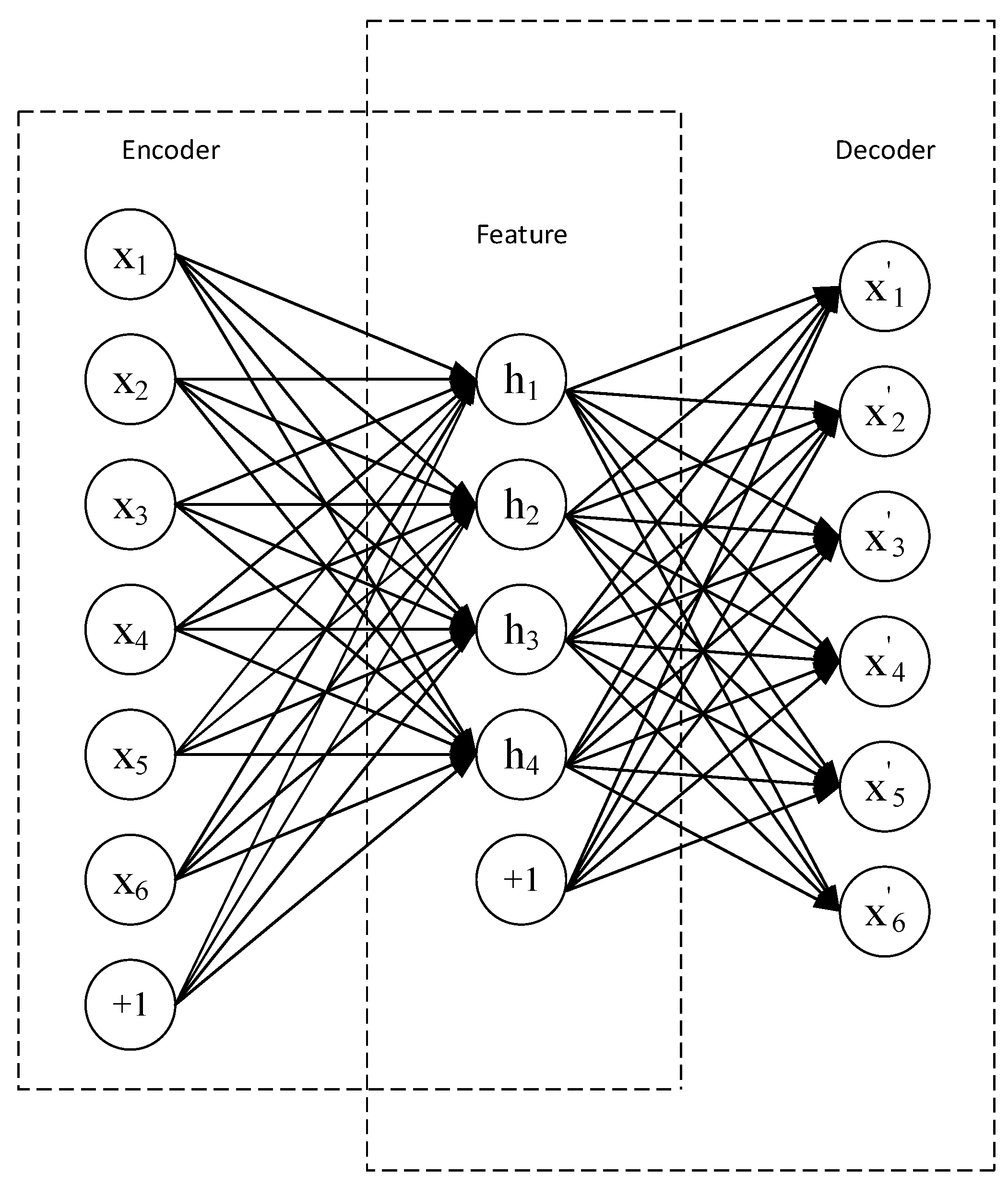
The autoencoder is an unsupervised learning algorithm whose output enables the reproduction of input data [23]. It is composed of two parts of neural network, namely the encoding part and the decoding part. The basic autoencoder can be thought of as a three-layer neural network structure: the input layer, the hidden layer, and the output layer. Figure 1 shows the structure of a basic autoencoder.

In previous neural networks, the input sample was usually labeled, so the parameters of the previous layers could be changed, according to the difference between the current output and the label, until convergence. Figure 2 shows the diagram of the training process with labeled samples. However, if the existing data is unlabeled, the previous method is not applicable. Figure 3 shows a diagram of an unlabeled sample training process. When the input x is sent to an encoder, an encoded output y is obtained. Here y is a representation of the input, but whether y is the input x is unknown, so a decoder is added, and then a decoded output z is obtained. The output z is compared with the input x. If z is very similar to x, there is reason to believe that y is reliable. Therefore, by adjusting the parameters of the encoder and decoder, the reconstruction error is minimized. At this time, the first representation of the input x is obtained, that is, y. Because the lidar data is unlabeled data, the source of the error is obtained directly by comparing the reconstructed data with the original input.

If the output y of the first layer is obtained, the minimum reconstructed error makes one believe that the output y is the approximation of original input signal x. Then there is no difference between the second and first layers of training. The output y of the first layer is regarded as the input signal of the second layer; minimizing the reconstruction error again can obtain both the parameters of the second layer and the encoded output of the second layer input, that is, the second expression of the original input information. Other layers can be obtained in the same way. Figure 4 shows the diagram of the stacking process.

The encoder function can be defined with Equation (2), and the decoder function can be expressed with Equation (3):

$$h=f_{\mathsf{\theta }}\left(x\right)={\delta }_1\left(W^{\left(1\right)}x+b^{\left(1\right)}\right)$$

(2)

$$g=f_{ \mathsf{\theta }\prime }\left(h\right)={\delta }_2\left(W^{\left(2\right)}h+b^{\left(2\right)}\right)$$

(3)

where x is the input lidar return signal, h is the main feature of the input data, g is the reconstructed lidar return signal, $W^{\left(1\right)}$ and $W^{\left(2\right)}$ are the weights of the encoder and decoder, $b^{\left(1\right)}$ and $b^{\left(2\right)}$ are the bias of the encoder and decoder, and ${\delta }_1$ and ${\delta }_2$ are the activation function of the encoder and decoder. In this paper, both encoder and decoder use the ReLU activation function [24].

2.3. One-Dimensional Convolution

For one-dimensional convolution, assuming that the input is a tensor $x^l\in R^{L^l\times D^l}$ and the convolution kernel of the current layer is a tensor $f^l\in R^{L^l\times D^l\times N}$, the one-dimensional convolution can be written by

$$y_{i^{l+1},d}=b_d+\sum _{i=0}^L\sum _{d=0}^{D^l}{f}_{i,d,n}^l\times x_{i^{l+1}+i,d}^l$$

(4)

where L is the size of the input data, D is the number of channels, N is the number of convolutions, n is the nth convolution, i is the coordinate of the value, d is the dth channel, and b is the bias. Convolution results can be represented as the sum of convolution at the appropriate location for all channels. Figure 5 shows the one-dimensional convolution calculation process. In this example the convolution kernel is $f\in R^{4\times 1\times 1}$ and input is $x\in R^{8\times 1}$. By zero filling on both sides of x (blue area) a new input $x^{\prime }\in R^{12\times 1}$ can be obtained; when convolution sliding stride 2, by performing a convolution operation of f on x, the output $y\in R^{5\times 1}$ will be obtained.

3. Principle of CAENN Algorithm

In this paper, the CAENN algorithm was constructed by combining the autoencoder and the one-dimensional convolutional neural network. Compared with the traditional autoencoder, the use of convolution processing instead of full connection is not only conducive to the extraction of data features, but also makes more effective use of the advantages of feature extraction of the autoencoder. The CAENN algorithm designed in this paper was able to extract the main lidar return signals from a relatively rich lidar data training set through the feature extraction process, layer by layer. Through the encoding–decoding process, the CAENN network was able to obtain the sparse expression of lidar return signals, and the original lidar return signal with a lot of noise was converted to lidar return signals with only effective signals, so as to filter out the noise, and then the clean lidar return signal was obtained by decoding part of reconstruction. Figure 6 shows the block diagram of the CAENN algorithm. Firstly, the lidar return signal is preprocessed by the normalization, and the preprocessed sample data is placed in the autoencoding layer of the CAENN algorithm for convolution and pooling encoding processing. Secondly, the detailed features of the sample data are encoded, and the noise is eliminated at the same time. Finally, using the decoding layer of the convolutional autoencoding network, the up-sampling and deconvolution are carried out. Deconvolution decodes the sampling features of the sample, which can recover the sample details and obtain a clean return signal.

3.1. Data Preprocessing

Since the measured lidar return signal values differ greatly, if they are directly sent to the network for training, it may cause numerical problems that will make the training model converge slowly or even not at all. Moreover, the convolutional neural network is relatively sensitive to the data distribution; if the distribution of training data and test data are different, the network training efficiency will decrease, the convergence will slow down, and the prediction effect will eventually be affected. Therefore, it is necessary to normalize the lidar return signal data before network training. According to the minimum value, after centering, the data a is scaled by the difference between the maximum value and the minimum value, then the data moves with the minimum unit and will be converged to [0, 1]. This process is called data normalization, which can be expressed with follow equation:

$$b=\frac{a-min\left(a\right)}{max\left(a\right)-min\left(a\right)}$$

(5)

The data normalization process can ensure that the data has a similar scale, which makes the model converge faster and improves the efficiency of network training.

3.2. Encoding Network

The encoding part of the CAENN algorithm is alternately composed of a convolutional layer, an activation function, and a down-sampling layer. The convolutional layer acts as a feature extractor to encode the lidar return signal and eliminate noise at the same time. In the convolutional layer, the convolution kernel of the current layer is convolved with the feature vector of the previous layer, and then the feature map of this layer is formed through the activation function. The output of the convolutional layer can be expressed as

$$H_1=x_n^l=f\left(m\sum _{m\in M_n}{x}_n^{l-1}\times w_{mn}^l+b_n^l\right)$$

(6)

where $x_n^l$ is the feature vector corresponding to the nth convolution kernel of the lth convolutional layer, $M_n$ represents the receptive domain of the current neuron, $w_{mn}^l$ represents the mth weighting coefficient of the nth convolution kernel of the lth layer, $b_n^l$ denotes the offset coefficient corresponding to the nth convolution kernel of the lth layer, and f is a nonlinear function. The encoding layer uses the ReLU activation function, which is defined as

$$ReLU\left(x\right)=max\{0,1\}=\{\begin{array}{c}x,x\ge 0\\ 0,x<0\end{array}$$

(7)

The down-sampling layer uses pooling technology to maintain features. Here, the maximum pooling operation is used to make features have scaling, displacement, and invariance. At the same time, the down-sampling layer has the function of secondary feature extraction and is expressed as

$$H_2=x_n^l=f\left({\beta }_n^l\times down\left(x_n^{l-1}\right)+b_n^l\right)$$

(8)

where down (·) means down-sampling, ${\beta }_n^l$ represents the weighting factor, and $b_n^l$ is the bias factor.

3.3. Decoding Network

The decoding part of the CAENN algorithm is alternately composed of up-sampling, the deconvolutional layer and the activation functions. The up-sampling is the reverse operation of down-sampling, that is, the up-pooling operation, which can solve the filter overlap problem in the deconvolutional process. The deconvolution is also called transposed convolution. This is because the forward propagation process of the convolutional layer is the back-propagation process of the deconvolutional layer, and the back-propagation process of the convolutional layer is the forward-propagation process of the deconvolutional layer. If the output features of the convolutional layer are up-sampling, the input features of the deconvolutional layer will be obtained. The up-sampling layer can be expressed as

$$H_3={x^{\prime }}_n^l=f\left({{\beta }^{\prime }}_n^l\otimes up\left({x^{\prime }}_n^{l-1}\right)+{b^{\prime }}_n^l\right)$$

(9)

where up (·) denotes up-sampling, $\otimes$ represents the up-sampling operation, ${{\beta }^{\prime }}_n^l$ is the weighting factor, and ${b^{\prime }}_n^l$ is the bias factor. The output of the lth deconvolution layer can be written as

$$H_4={x^{\prime }}_n^l=f\left(m\sum _{m\in M_n}{x^{\prime }}_n^{l-1}\otimes {w^{\prime }}_{mn}^l+{b^{\prime }}_n^l\right)$$

(10)

where ${x^{\prime }}_n^l$ is the feature vector corresponding to the nth deconvolution kernel of the lth convolutional layer, $M_n$ is the receptive domain of the current neuron, $\otimes$ is the deconvolution operation, ${W^{\prime }}_{mn}^l$ is the mth weighting coefficient of the nth deconvolution kernel of the lth layer, ${b^{\prime }}_n^l$ is the offset coefficient corresponding to the nth deconvolution kernel of the lth layer, and f (·) is a nonlinear function. The decoding layer also uses the ReLU activation function.

3.4. Model Parameters

In this paper, the CAENN model parameters were set by several comparison experiments, for example, the number of convolutional layers, pooling layers and up-sampling layers, the convolution kernel size, and the step size, and other parameters of the one-dimensional convolutional layer were adjusted.

Table 1. The comparison experiment of activation function.

Activation Function	Training Time	SNR	MSE
ReLU	3 h 8 min	12.4673	4.0178 × 10−7
Tanh	3 h 27 min	11.9523	4.5238 × 10−7

,

Table 2. The comparison experiment of the number of convolutional layers.

Number of Convolutional Layers	SNR	MSE
Two layers	11.28405	5.2760 × 10−7
Three layers	19.2726	8.3842 × 10−8
Four layers	14.6482	2.4316 × 10−7
Five layers	13.9446	2.8593 × 10−7

and

Table 3. The comparison experiment of the learning rate.

Learning Rate	SNR	MSE
0.1	15.7745	1.8753 × 10−7
0.01	16.6819	1.5224 × 10−7
0.005	17.5551	1.2451 × 10−7
0.001	17.7745	1.1837 × 10−7

shows the SNR and MSE of the comparison experiments including the activation function, the number of convolutional layers and the learning rate. From these tables we can conclude the optimal structure and parameters: it used the ReLU activation function, the network structure was composed of three convolutional layers with one down-sampling layer or one up-sampling layer alternately, batch size was set to 128, learning rate was set to 0.001, epochs were set to 500, and early stopping was used, which involved stopping training when the model’s performance on the validation set started to decline, in order to avoid the problem of over-fitting caused by continuing training.

Table 4. The parameters of CAENN method.

Layer (Type)	Output Shape
Input_1(InputLayer)	(None, 8800, 1)
conv1d(Conv1D)	(None, 8800, 128)
conv1d_1(Conv1D)	(None, 8800, 64)
conv1d_2(Conv1D)	(None, 8800, 64)
max_pooling1d(MaxPooling1D)	(None, 4400, 64)
conv1d_3(Conv1D)	(None, 4400, 32)
conv1d_4(Conv1D)	(None, 4400, 32)
conv1d_5(Conv1D)	(None, 4400, 16)
max_pooling1d _1(MaxPooling1D)	(None, 2200, 16)
conv1d_6(Conv1D)	(None, 2200, 16)
conv1d_7(Conv1D)	(None, 2200, 32)
conv1d_8(Conv1D)	(None, 2200, 32)
up_sampling1d(UpSampling1D)	(None, 4400,32)
conv1d_8(Conv1D)	(None, 4400, 64)
conv1d_10(Conv1D)	(None, 4400, 64)
conv1d_11(Conv1D)	(None, 4400, 128)
up_sampling1d_1(UpSampling1D)	(None, 8800, 128)
conv1d_12(Conv1D)	(None, 8800, 1)

lists the optimal CAENN parameters by comparison experiments. The run time in this experiment was only obtained under the follow computer configuration: Intel(R) Core(TM) i5-10210U CPU, Windows10 operating system, RAM 8 GB, and GeForce MX250. Due to the low computer configuration, it took 5 h 38 m 40.508626 s to train the model, but it only took 2.174187 s to use the trained model to test a set of data.

3.5. Adam Optimization Algorithm

In view of the problem we want to address, the mean-square error (MSE) is selected as the loss function by comparison, and the network parameters are estimated by minimizing the MSE loss function. Assuming $x_n$ is the original data, the objective function is designed to optimize the objective function through the original data and the reconstructed data ${\hat{x}}_n$, where n is the number of training samples, and the loss function is expressed as

$$L(\mathsf{\theta })=\frac{1}{n}\sum _{i=1}^n\parallel x_n-{\widehat{x}}_n\parallel {}^2$$

(11)

Stochastic gradient descent (SGD) is one of the most commonly used gradient descent methods for optimizing neural networks. However, there are some problems in this training method, such as the selection of learning rate and the oscillation problem during updating. It is often difficult to select an appropriate learning rate, which intensifies the difficulty of training to minimize the objective function. In this paper, the Adam algorithm is used instead of the stochastic gradient descent method for updating the network parameters. The essence of the Adam optimization algorithm is to combine the first-order momentum with the second-order momentum and then correct the deviation. The Adam operator automatically calculates the appropriate learning rate for each parameter, which solves the problem of the stochastic gradient descent method that makes it difficult to choose the learning rate. When the Adam operator is used to solve the weight of a certain neuron, the update process of the θ value after the tth iteration is written as

$$m_t={\beta }_1{m}_{t-1}+\left(1-{\beta }_1\right)g_t$$

(12)

$$n_t={\beta }_2{n}_{t-1}+\left(1-{\beta }_2\right)g_t^2$$

(13)

where $g_t$ is the first order derivative, ${\beta }_1$ and ${\beta }_2$ are the attenuation factor which controls the exponential attenuation, $m_t$ is the exponential moving average value of the gradient obtained from the first moment of the gradient, and $n_t$ is the square gradient obtained from the second moment of the gradient. At this point, both $m_t$ and $n_t$ are biased estimates, each of which must be corrected to become an unbiased estimate of expectations.

$${\widehat{m}}_{\mathrm{t} }=\frac{m_t}{1-{\beta }_1^t}$$

(14)

$${\widehat{n}}_t=\frac{n_t}{1-{\beta }_2^t}$$

(15)

The corrected $m_t$ and $n_t$ can dynamically update the learning rate, and the last formula for parameter updates is written as

$${\mathsf{\theta }}_{l+1}={\mathsf{\theta }}_t-\frac{{\widehat{m}}_t}{\sqrt{{\widehat{n}}_t+\epsilon }}\eta$$

(16)

where, η is the learning rate. The Adam optimization algorithm can adaptively adjust the updated step size from the two aspects of the gradient mean and the gradient square, instead of being directly determined by the current gradient. The Adam optimization algorithm initializes the parameter vector, the first-order moment vector and the second-order moment vector at first, and then iteratively updates each part to make the parameter θ converge.

4. Results and Analysis

4.1. Noise Reduction Effect Evaluation

In order to evaluate the effect of denoising algorithm, both the signal-to-noise ratio (SNR) and MSE are generally adopted for evaluation [25]. The SNR is the ratio relationship between signal and noise, and reflects the noise reduction effect. The higher the value, the better the effect of noise elimination. The MSE represents the relationship between the original signal and the denoised signal, and the smaller the value is, the better the effect is. The SNR and MSE are expressed with follow equations:

$$SNR=10log\left(\frac{{\sum }_{i=1}^N{x}_i{}^2}{{\sum }_{i=1}^N{\left(x_i-{\tilde{x}}_i\right)}^2}\right)$$

(17)

$$MSE=\frac{1}{N}\sum _{i=1}^N{\left(x_i-{\tilde{x}}_i\right)}^2$$

(18)

where $x_i$ is the original signal, ${\tilde{x}}_i$ is the signal after denoising, and N is the signal length.

4.2. Simulation Verification

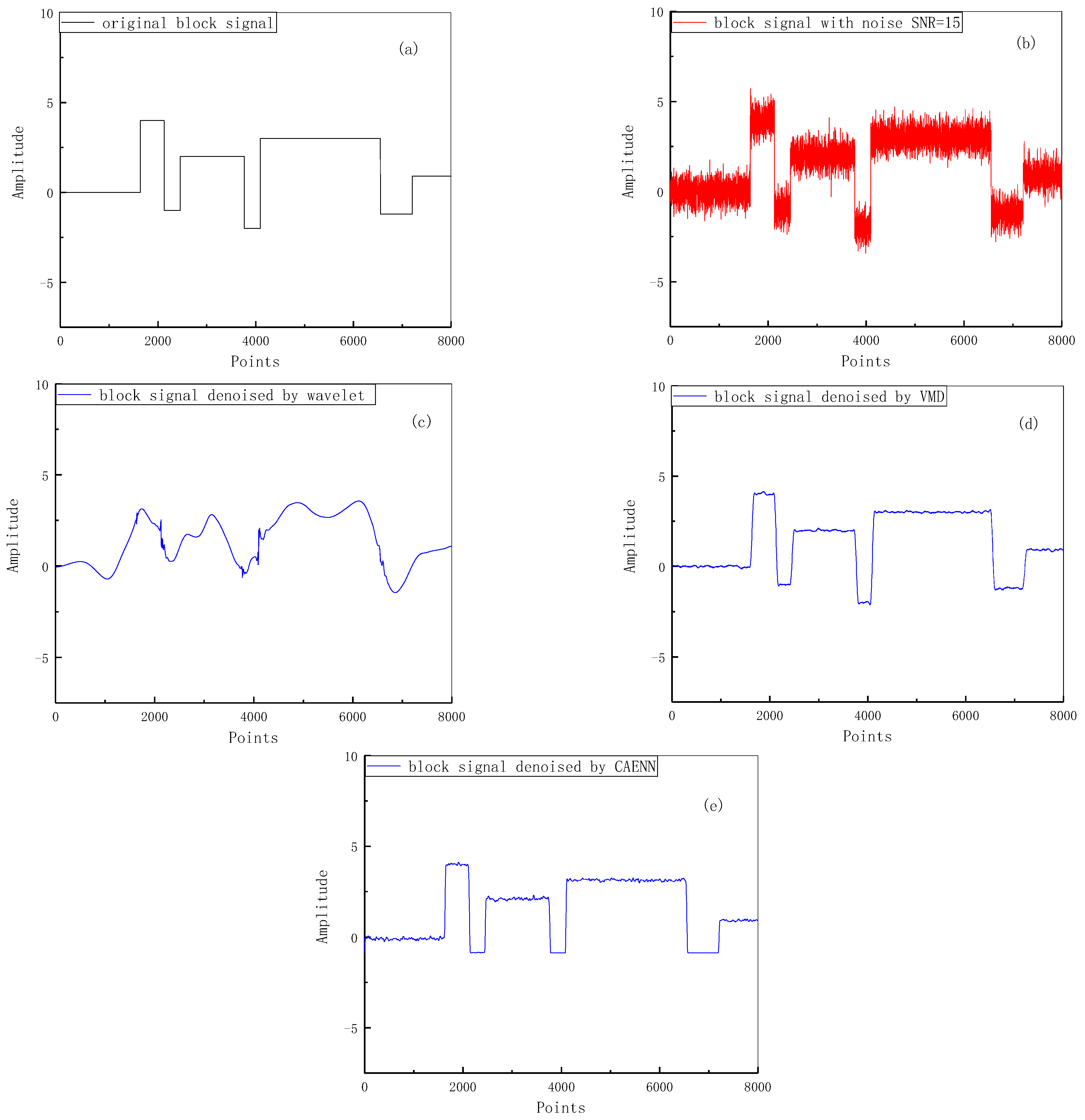
The interference noise of the lidar return signal mainly includes background radiation noise, shot noise, dark current noise of the detector, and thermal radiation noise. In order to verify the effectiveness and superiority of the CAENN method, the signal containing gaussian white noise is simulated, also a result comparison of CAENN method with wavelet threshold method and VMD method is performed [26]. In this paper, the Block test signal and Bump test signal proposed by Donoho and Johnstone were superimposed with Gaussian white noise, and the two test signals were denoised by the CAENN, wavelet threshold and VMD methods, respectively [27].

In a real environment, noise is often a complex phenomenon from many different sources. Assuming that real noise is regarded as the sum of many random variables with different probability distributions, and that each random variable is independent, their normalized sum tends to Gaussian distribution with the increase in the number of noise sources according to the Central Limit Theorem. In this paper, the Gaussian white noise with SNR = 15 was added to both the Block test signal and the Bump test signal. The purpose of adding noise with a specified SNR in the simulation experiment was to quantify and evaluate the effect of the algorithm. The wavelet threshold denoising method used db8 wavelet basis function for nine-layer decomposition; the VMD used three-layer decomposition; the CAENN used a self-made data set for training, batch size was 128, and epoch was set to 500. When the model is not optimized 10 consecutive times, it will end early. Figure 7 and Figure 8 show the simulated noise reduction effects for Block and Bump signals, respectively. It can be seen that the three noise reduction methods all had a certain noise reduction effect. The wavelet threshold method filtered out almost all noise, but the processed Block signal and the Bump signal produced significant distortions compared to the unprocessed signal, and this effect was the worst. The VMD method had a better denoising effect and better signal detail retention, but distortion also appeared to some extent. The CAENN method had the best denoising effect and retained the signal details very well.

In order to further evaluate the effects of three denoising methods mentioned above, the SNR and MSE of the denoised Block signal and Bump signal were calculated, respectively, when superimposed with Gaussian white noise with different SNRs of 5 dB, 10 dB and 15 dB.

Table 5. The SNR and MSE after noise reduction by three methods when superimposed with noise with different SNRs.

Signal	SNRnoise	Wavelet Threshold		VMD		CAENN
		SNR	MSE	SNR	MSE	SNR	MSE
Block	5 dB	5.1068	1.6028	8.2578	0.7966	17.8960	0.0711
	10 dB	6.6237	1.0074	12.4210	0.2652	19.8413	0.0454
	15 dB	7.2619	0.8391	15.2248	0.1341	20.7961	0.0364
Bump	5 dB	6.3831	1.1887	8.1213	0.7966	19.5454	0.0475
	10 dB	8.7042	0.6239	12.5492	0.2533	25.3450	0.0125
	15 dB	10.1135	0.4266	17.3844	0.0799	23.0537	0.0212

lists the SNR and MSE after noise reduction by three methods when superimposed with noise with different SNRs.

It is clear that although the weak noise remains, the SNR of the CAENN noise reduction method is nearly twice that of the other two methods, and the MSE of the CAENN method is less than one-tenth of that of the other two methods.

4.3. Denoising Effect of Actually Measured Lidar Signals

The actual signals used in this paper were all detected by a small Mie-scattering lidar developed at North Minzu University (106°06′ E, 38°29′ N). The system parameters of the Mie-scattering lidar are shown in

Table 6. The system parameters of Mie scattering lidar.

Parameters	Parameters Index
Laser	Nd:YAG laser
Wavelength	1064 nm, 532 nm, 355 nm
Single pulse energy	350 mJ@1064 nm, 170 mJ@532 nm, 80 mJ@355 nm
Impulse frequency	1–10 Hz
Pulse width	≤10 ns@1064 nm
Beam diameter	~9 mm@1064 nm
Divergence angle	≤0.5 mrad@1064 nm
Telescope	Schmidt–Cassegrain type
Diameter	300 mm
Field of view angle	0.4 mrad
Horizontal angle	0–360°
Pitching angle	0–90°
Detection range	100–13,000 m (Night), 100–10,000 m (Daytime)

. The data set used to train the network consisted of a total of 830 sets of data, including sunny, cloudy, cloudy, sandy, and other weather data, of which 90% were used for training and 10% were used for testing. Every collected original signal had a total of 10,000 data points, and the first 1000 data points were background noise, which was able to be used to calculate the average noise of the data acquisition system and was subtracted in the data preprocessing. Therefore, the starting point of the calculation was set to 1000.

Figure 9 shows the aerosol extinction coefficient profiles at a wavelength of 532 nm retrieved by the Klett method and the corresponding denoising effect. In Figure 9a, the original signal contains a lot of noise, and the useful signal is almost completely submerged in the noise above the height of 6 km. Figure 9b shows the aerosol extinction coefficient profile processed by the wavelet threshold method. Although the noise is filtered out, the signal details are seriously lost at the height of more than 8 km. In Figure 9c, the aerosol extinction coefficient profile is processed by the VMD method. Its noise reduction effect and signal detail retention are better than the wavelet threshold method, however, compared with the denoising method based on the CAENN method, the signal details are also lost to a certain extent. In Figure 9d, the aerosol extinction coefficient profile is processed by the CAENN method. Although the curve is rough, the details are well maintained. In order to quantitatively evaluate the denoising effect of these three methods, the SNR and MSE were calculated, as listed in

Table 7. The SNR and MSE of lidar signals denoised by three methods shown in Figure 9.

	Wavelet Threshold	VMD	CAENN
SNR	19.8002	20.5140	21.4392
MSE	6.4828 × 10−7	6.1008 × 10−7	5.68 × 10−7

. It can be seen that the SNR of the method proposed in this paper was higher than the other two, while the MSE was lower than the other two, and the denoising effect was the best.

In order to further verify the denoising effect of the three methods for complex lidar signals, the extinction coefficient profiles containing cloud layer were employed for our goal. Figure 10 and Figure 11 show the aerosol extinction coefficient profiles and denoising effect inverted by the Klett method. Compared with Figure 9, the two groups of signals have obvious cloud layers. In Figure 10a and Figure 11a, the original signals contain a lot of noise. The useful signals are almost completely submerged in the noise above the height of 5 km. In Figure 10a, there is a cloud layer with a thickness of 1 km between 3 km and 4 km, and its extinction coefficient has reached 0.011 km⁻¹. However, in Figure 11a, a cloud layer with a thickness of 1 km appears at the height of 3 km to 4 km with an extinction coefficient of 0.049 km⁻¹; in addition, there is another cloud layer with a thickness of 2 km at the height of 4 km to 6 km with an extinction coefficient of 0.038 km⁻¹. In Figure 10b and Figure 11b, the aerosol extinction coefficient profiles are processed by the wavelet threshold method. Although the curves are very smooth and almost all the noise is filtered out, there are some significant distortions, especially at the peaks of the clouds, and the extinction coefficient value shows an obvious change compared with the original signals shown in Figure 10a and Figure 11a. In Figure 10c and Figure 11c, the aerosol extinction coefficient profiles are processed by the VDM method. The effect of noise reduction and signal detail retention are better than the wavelet threshold method. In Figure 10d and Figure 11d, the aerosol extinction coefficient profiles are processed by the CAENN method. Although the curves are relatively rough, the details are maintained well. Moreover, this method does not achieve its denoising effect at the cost of the spatial resolution and distortion. Meanwhile, comparing VDM with the CAENN method, the signal details denoised by VDM method are lost to a certain extent. In order to evaluate further the processing effects of these three methods on the two groups of signals, the corresponding SNRs and MSEs were calculated respectively.

Table 8. The SNR and MSE of signals denoised by three methods shown in Figure 10.

	Wavelet Threshold	VMD	CAENN
SNR	12.7456	14.1889	14.8419
MSE	3.7665 × 10−7	2.6921 × 10−7	2.0179 × 10−7

and

Table 9. The SNR and MSE of signals denoised by three methods shown in Figure 11.

	Wavelet Threshold	VMD	CAENN
SNR	16.7403	17.9197	18.8352
MSE	1.3339 × 10−5	9.0192 × 10−6	8.4257 × 10−6

list the SNR and MSE of signals denoised by three methods shown in Figure 10 and Figure 11, respectively. It can be seen that the SNRs of the CAENN method proposed in this paper are higher than the other two, while the MSEs are lower than the other two, and the denoising effects are the best.

4.4. Discuss

As seen in the simulation and measured data verification above, the denoising effect of the wavelet threshold method is the least effective among the three methods. The processed signal has significant distortion and the signal peak has a certain proportion of scaling. This denoising algorithm at the expense of signal fidelity is not desirable in practical applications. The VMD method is better than the wavelet threshold method in denoising effect and signal fidelity. However, the signal decomposition effect of VMD depends to a certain extent on the number of decomposition layers and the penalty factor, but these two parameters must be selected manually. It is usually difficult to obtain the optimal combination of these two parameters, and the adaptive ability is poor. The algorithm proposed in this paper has strong adaptive ability, and its excellent denoising effect can be easily seen through the calculation of SNR and MSE. Because the number of signals with clouds in the training data set is small at present, the signal reconstructed by the model for the cloud signals contains a small amount of noise. If adding more data with clouds for training, the network learning ability and refactoring capability can be improved further, and the denoising effect will be improved well.

5. Conclusions

In this paper a method for denoising lidar return signals based on the CAENN method is proposed, which uses the encoding and decoding characteristics of the autoencoder to extract the deep features of lidar return signals layer by layer by constructing convolutional neural networks. Through the encoding–decoding process, the CAENN network can obtain the sparse expression of lidar return signals, which can convert the original lidar return signals with a lot of noise to lidar return signals with only effective signals, so as to filter out the noise. The encoding part extracts the features through the convolutional network, and eliminates the noise at the same time, while the decoding part completes the reconstruction of the data. To verify the feasibility of the method proposed, some simulations and experiments were carried out. The results show that the signal processed by CAENN method has the highest SNR ratio and the smallest MSE compared with the wavelet threshold and VMD methods, and its denoising effect is the most obvious. The algorithm proposed in this paper has strong adaptive ability, and its excellent denoising effect can be easily seen through the calculation of SNR and MSE. However, due to the scarcity of data involving special weather among the data sets, the processing of such data may lead to a small amount of noise remaining in the reconstructed signal. In future, we will collect more lidar signals in special weather to expand the data sets in order to train the network and optimize the model, thus further improving the universality of the model. This proposed method effectively improves the SNR of the lidar return signal, while retaining the complete characteristics of the signal, proving its effectiveness in denoising the lidar return signal.

References

1. Fang, H.T.; Huang, D.S.; Wu, Y.H. Antinoise approximation of the lidar signal with wavelet neural networks. Appl. Opt. 2005, 44, 1077–1083. [Google Scholar] [CrossRef] [PubMed]
2. Wu, S.; Liu, Z.; Liu, B. Enhancement of lidar backscatters signal-to-noise ratio using empirical mode decomposition method. Opt. Commun. 2006, 267, 137–144. [Google Scholar] [CrossRef]
3. Mao, J.; Hua, D.; Wang, Y.; Wang, L. Noise Reduction in Lidar Signal Based on Wavelet Packet Analysis. China J. Lasers 2011, 38, 226–233. [Google Scholar]
4. Qin, X.; Mao, J. Noise reduction for lidar returns using self-adaptive wavelet neural network. Opt. Rev. 2017, 24, 416–427. [Google Scholar] [CrossRef]
5. Huang, N.E.; Shen, Z.; Long, S.R.; Wu, M.C.; Shih, H.H.; Zheng, Q.; Yen, N.C.; Tung, C.C.; Liu, H.H. The empirical mode decomposition and the Hilbert spectrum for nonlinear and non-stationary time series analysis. Proc. Math. Phys. Eng. Sci. 1998, 454, 903–995. [Google Scholar] [CrossRef]
6. Zheng, F.; Hua, D.; Zhou, A. Empirical Mode Decomposition Algorithm Research & Application of Mie Lidar Atmospheric Backscattering Signal. China J. Lasers 2009, 36, 1068–1074. [Google Scholar]
7. Cheng, X.; Mao, J.; Li, J.; Zhao, H.; Zhou, C.; Gong, X.; Rao, Z. An EEMD-SVD-LWT algorithm for denoising a lidar signal. Measurement 2021, 168, 108405. [Google Scholar] [CrossRef]
8. Dragomiretskiy, K.; Zosso, D. Variational Mode Decomposition. IEEE Trans. Signal Process. 2014, 62, 531–544. [Google Scholar] [CrossRef]
9. Xu, F.; Chang, J.; Liu, B.; Li, H.; Zhu, L.; Dou, X. De-noising method research for lidar return signal based on variational mode decomposition. Laser Infrared 2018, 48, 1443–1448. [Google Scholar]
10. Marais, W.J.; Holz, R.E.; Hu, Y.H.; Kuehn, R.E.; Eloranta, E.E.; Willett, R.M. Approach to simultaneously denoise and invert backscatter and extinction from photon-limited atmospheric lidar observations. Appl. Opt. 2016, 55, 8316–8334. [Google Scholar] [CrossRef]
11. Marais, W.; Willett, R. Proximal-Gradient methods for poisson image reconstruction with BM3D-Based regularization. In Proceedings of the 2017 IEEE 7th International Workshop on Computational Advances in Multi-Sensor Adaptive Processing (CAMSAP), Curaçao, The Netherlands, 10–13 December 2017; pp. 1–5. [Google Scholar]
12. Hayman, M.; Stillwell, R.; Spuler, S. Optimization of linear signal processing in photon counting lidar using Poisson thinning. Opt. Lett. 2020, 45, 5213–5216. [Google Scholar] [CrossRef]
13. LeCun, Y.; Bengio, Y.; Hinton, G. Deep learning. Nature 2015, 521, 436–444. [Google Scholar] [CrossRef] [PubMed]
14. García-Gutiérrez, J.; González-Ferreiro, E.; Mateos-García, D.; Riquelme-Santos, J.C. A preliminary study of the suitability of deep learning to improve LiDAR-derived biomass estimation. In International Conference on Hybrid Artificial Intelligence Systems; Springer: Cham, Switzerland, 2016; pp. 588–596. [Google Scholar]
15. Sleeman, J.; Halem, M.; Yang, Z.; Caicedo, V.; Demoz, B.; Delgado, R. A Deep Machine Learning Approach for LIDAR Based Boundary Layer Height Detection. In Proceedings of the IGARSS 2020—2020 IEEE International Geoscience and Remote Sensing Symposium, Waikoloa, HI, USA, 26 September–2 October 2020; pp. 3676–3679. [Google Scholar]
16. Andreas, A.; Brain, S.; Andrew, M. Deep learning for LiDAR waveforms with multiple returns. In Proceedings of the 2020 28th European Signal Processing Conference (EUSIPCO), Amsterdam, The Netherlands, 18–21 January 2021; pp. 1571–1575. [Google Scholar]
17. Hinton, G.E.; Salakhutdinov, R.R. Reducing the Dimensionality of Data with Neural Networks. Science 2006, 313, 504–507. [Google Scholar] [CrossRef] [Green Version]
18. Chen, J.; Liu, M.; Xiong, P.; Meng, X.; Yang, L. ECG signal denoising based on convolutional auto-encoder neural network. Comput. Eng. Appl. 2020, 56, 148–155. [Google Scholar]
19. Masci, J.; Meier, U.; Cireşan, D.; Schmidhuber, J. Stacked Convolutional Auto-Encoders for Hierarchical Feature Extraction. In International Conference on Artificial Neural Networks; Springer: Berlin/Heidelberg, Germany, 2011; pp. 52–59. [Google Scholar]
20. Collis, R.T.H. Lidar: A new atmospheric probe. Q. J. R. Meteorol. Soc. 2010, 92, 220–230. [Google Scholar] [CrossRef]
21. Klett, J.D. Stable analytical inversion solution for processing lidar returns. Appl. Opt. 1981, 20, 211–220. [Google Scholar] [CrossRef] [Green Version]
22. Fernald, F.G. Analysis of atmospheric lidar observations: Some comments. Appl. Opt. 1984, 23, 652–653. [Google Scholar] [CrossRef]
23. Jia, W.; Zhang, Y. Survey on Theories and Methods of Autoencoder. Comput. Syst. Appl. 2018, 27, 1–9. [Google Scholar]
24. He, K.; Zhang, X.; Ren, S.; Sun, J. Delving Deep into Rectifiers: Surpassing Human-Level Performance on ImageNet Classification. In Proceedings of the IEEE International Conference on Computer Vision, Santiago, Chile, 7–13 December 2015; p. 123. [Google Scholar]
25. Zhou, Z.; Hua, D.; Wang, Y.; Yan, Q.; Li, S.; Li, Y.; Wang, H. Improvement of the signal to noise ratio of Lidar return signal based on wavelet de-noising technique. Opt. Lasers Eng. 2013, 51, 961–966. [Google Scholar] [CrossRef]
26. Zhou, Z.; Hua, D.; Yang, R.; Yan, Q.; Chen, H.; Song, Y. De-noising Method for Mie Scattering Lidar Echo Signal Based on Wavelet Theroy. Acta Photonica Sin. 2016, 45, 70701002. [Google Scholar] [CrossRef]
27. Zhang, Y.K.; Ma, X.C.; Hua, D.X.; Chen, H.; Liu, C.X. The Mie Scattering Lidar Return Signal Denoising Research Based on EMD-DISPO. Spectrosc. Spectr. Anal. 2011, 31, 2996–3000. [Google Scholar]
Figure 1. The structure of a basic autoencoder.
Atmosphere 12 01403 g001
Figure 2. The diagram of the training process with labeled samples.
Atmosphere 12 01403 g002
Figure 3. The diagram of the training process with unlabeled samples.
Atmosphere 12 01403 g003
Figure 4. The diagram of stacking the process.
Atmosphere 12 01403 g004
Figure 5. The one-dimensional convolution calculation process.
Atmosphere 12 01403 g005
Figure 6. The block diagram of the CAENN algorithm.
Atmosphere 12 01403 g006
Figure 7. The simulated noise reduction effects of Block signals. (a) the original block signal, (b) the block signal with SNR = 15 noise, (c) the signal processed by the wavelet threshold method, (d) the signal processed by the VMD method, (e) the signal processed by CAENN method.
Atmosphere 12 01403 g007
Figure 8. The simulated noise reduction effects of Bump signals. (a) the original bump signal, (b) the bump signal with SNR = 15 noise, (c) the signal processed by the wavelet threshold method, (d) the signal processed by the VMD method, (e) the signal processed by CAENN method.
Atmosphere 12 01403 g008
Figure 9. The aerosol extinction coefficient profiles obtained by the Klett method and its denoising effect at a wavelength of 532 nm. (a) the original signal, (b) the signal processed by the wavelet threshold method, (c) the signal processed by the VMD method, (d) the signal processed by CAENN method.
Atmosphere 12 01403 g009
Figure 10. The aerosol extinction coefficient profiles containing a cloud layer obtained by the Klett method and its denoising effect at a wavelength of 532 nm. (a) the original signal, (b) the signal processed by the wavelet threshold method, (c) the signal processed by the VMD method, (d) the signal processed by CAENN method.
Atmosphere 12 01403 g010
Figure 11. The aerosol extinction coefficient profiles containing two cloud layers obtained by the Klett method and its denoising effect at a wavelength of 532 nm. (a) the original signal, (b) the signal processed by the wavelet threshold method, (c) the signal processed by the VMD method, (d) the signal processed by CAENN method.
Atmosphere 12 01403 g011