Article

A Non-Stationary Heat Spell Frequency, Intensity, and Duration Model for France, Integrating Teleconnection Patterns and Climate Change

by
Yasser Hamdi
1,*,
Christian Charron
2 and
Taha B. M. J. Ouarda
2
1
Institute for Radiological Protection and Nuclear Safety, CEDEX BP17, 92262 Fontenay-aux-Roses, France
2
Centre Eau Terre Environnement, Institut National de la Recherche Scientifique, Québec, QC G1K9A9, Canada
*
Author to whom correspondence should be addressed.
Atmosphere 2021, 12(11), 1387; https://doi.org/10.3390/atmos12111387
Submission received: 25 August 2021 / Revised: 11 October 2021 / Accepted: 14 October 2021 / Published: 22 October 2021
(This article belongs to the Special Issue Extreme Climate Events in France)

Abstract

:
The warming observed over the past summers since 2000 is unprecedented in climate records in Europe and especially in France. Extreme temperatures and heat spells were often analyzed in the literature by applying extreme value theory but rarely in a non-stationary (NS) framework and duration modeling is often excluded. For a modern risk-based approach, it is important to have knowledge of the duration, magnitude, and frequency of occurrence of heat spells in a climate variability and change context. Yet, despite their obvious importance, teleconnections and associated climate indices (CIs) have often been excluded from heat spell modelling. The notion of duration is also not easily interpretable in a frequency analysis and can even be subtle, especially in a NS context. In this study, we used time-varying statistical distributions with parameters conditional on covariates representing the time and CIs. The daily maximum temperatures (DMTs) observed at the Orange and Dijon stations in France were used as a case study. This paper highlights a possible relationship between some large-scale climate patterns and the heat spells in France. Overall, the results suggest that considering the combined effect of global warming and these patterns in NS models is useful for a more appropriate characterization of the hazard heat spells in France.

1. Introduction

It is well established today that Europe has been rapidly warming since the late 1970s [1,2]. Concurrently, extreme weather events have become more frequent over many areas in Europe [3]. In this context, France has become more prone to experiencing extended summertime spells of exceptionally hot weather, which can have major impacts on the environment, public health, and population safety. For instance, several European countries experienced exceptionally hot weather during the summer of 2019 and, as shown in Figure 1, record temperatures were expected across Europe on 25 July, during which much of France then received a red alert (the highest level of warning). Comparisons have been made between that event and a heat wave that France experienced in August 2003 [4], which was responsible for massive excess mortality (almost 15,000 deaths) and tremendous socioeconomic impacts [5,6,7]. That unprecedented heat wave also had significant adverse impacts across Europe: in an unprecedented move, Belgium had issued a code red weather warning for the whole country. A red alert was declared in some regions in Spain, some of which were already subject to devastating wildfires one month earlier. In the Netherlands and in the UK, the governments had activated their “national heat plans”.
Over 80% of the electricity in France is derived from nuclear power. Nuclear energy is known to be one of the poorest greenhouse gas emitters, but, paradoxically, global warming is making the technology more vulnerable. As nuclear power plants (NPPs) need large amounts of water for cooling purposes and around two thirds of France’s 56 nuclear reactors obtain their water supplies from nearby rivers, electricity generation through these NPPs is threatened by heat spells. Indeed, once the cooling of the reactors is completed, the warmed water is discharged back into the rivers. In addition, droughts, which can be caused by hot weather, can lower water levels in rivers and increase water temperature. This situation is contrary to the French regulations which stipulate that in order to protect plants and animal life, power generation must be cut when water temperature is relatively high (increases above 28 °C for some NPPs) or when river water levels are low. Just during the summer of 2019, two intense heat spells swept through Europe, establishing it as the hottest summer on record in many areas. In France, scorching temperatures led the French Electricity Operator (EDF: Électricité de France) to shut down the Golfech reactors and to decrease the power of some other NPPs. Furthermore, the risk of failure of sensitive equipment in NPPs is also increased due to heat spells if they are more intense and frequent. Despite the fact that NPPs in France were constructed to withstand hot weather and in spite of all the efforts made by operators to protect NPPs against extreme temperatures and heat spells, the impact of climate variability and change remains an important issue for the Institute for Radiological Protection and Nuclear Safety (IRSN).
Increases in extreme temperature indices since the middle of the twentieth century have been reported in a number of studies [8,9,10,11,12]. The increases in extreme temperature events have been largely attributed to global warming, which is at about 0.6 °C globally since 1951–1980 [13]. Many studies emphasize that due to urbanization and industrialization, and in the context of climate change, the frequency, intensity, and duration of heat spells are likely to increase in the future based on climate change scenarios (e.g., [14,15,16]). France has not been spared by this warming and studies have no doubt that climate change and the increase in both the intensity and frequency of hot weather events are very real [1,17,18]. Since 2003, particularly intense heat spells have hit several other areas of the world (Russia, 2010; Texas, 2011; Australia, 2012; and Spain, 2015), while France has been confronted with less intense events, apart from in 2003, although increasingly frequent (July, 2006; August, 2012; July, 2013; July, 2015; August, 2016; June, 2017; July and August, 2018; and June and July, 2019). In 2019, a large number of records were broken, in particular, by exceeding the temperatures measured in 2003 on more than half of the stations.
According to Meteo-France, future climate projections also seem to support an increasing trend in temperature extremes over France [17]. Authors stated “Under future climate conditions, whatever the considered scenario, the heat waves become more frequent and have higher mean duration and intensity. Moreover, heat waves could occur during a larger part of summer”. In a 2014 study conducted in France [19], it was concluded that the expected rise in average temperatures, at a relatively close horizon (2021–2050), is about 0.6–1.3 °C compared to those calculated over the reference period. This increase is expected to be greater in south-eastern France in the summer, with deviations from the reference value of up to 1.5–2.0 °C. For the same time period, the duration of heat spells in the summertime will increase by up to five days throughout France and this increase will reach 10 days in south-eastern France. The average temperatures during summer are likely to increase over a longer term (2071–2100). The expected rise varies according to the scenarios injected into the climate models and it should be particularly pronounced in south-eastern France as well as may significantly exceed 5 °C in the summertime compared to the reference average. The RCP2.6 and RCP8.5 (business as usual) scenarios indicate an increase of up to 1.3 °C and 5.3 °C, respectively. The duration of heat spells will increase for the same time period and could exceed 20 days in the south-eastern part of France. Climate warming in France has been a topic of increasing interest and several other studies and projects have been carried out on both a Europe-wide scale and in France: PRUDENCE (2001–2004), Imfrex (2003–2005), Extremoscope (2013–2016), etc.
The geographic location of the site (latitude and longitude) and other physiographic characteristics (altitude, distance to the ocean, land cover, urbanization, percentage of forest, percentage of area covered by lakes, etc.) have a direct impact on heat spell characteristics. It has also been argued in several studies that, apart from these local factors, the influence of large-scale oscillation patterns on the climate in France is not minor. The Atlantic Multidecadal Oscillation (AMO) has a significant influence on the climate of the Northern Hemisphere. It is defined by the low frequency fluctuation of the sea surface temperature (SST) over the North Atlantic basin with wide-ranging impacts on a global scale. It has been shown to be linked to the warming in France during the last 15–20 years, which is due to the exchange of energy between the ocean and the atmosphere. Milenković et al. [20] established connections between the AMO and forest fires in France during the period of 1980–2014. Giuntoli et al. [21] demonstrated that the North Atlantic Oscillation (NAO) and the AMO with other weather patterns (associated to wet and dry conditions) have a significant influence on heat spells in France (https://www.encyclopedie-environnement.org/en/climate/extreme-weather-events-and-climate-change/, accessed 15 May 2021). NAO is a large-scale alternation of atmospheric mass between subtropical high surface pressure, centered on the Azores, and subpolar low surface pressure, centered on Iceland. The authors stated that these large-scale patterns are responsible for the increase of drought severity in southern France. The third mode of variability examined in this study is the Pacific-North American pattern (PNA). It is also one of the most prominent modes of low-frequency variability and large-scale weather patterns in the Northern Hemisphere extratropics [22,23]. PNA relates the atmospheric circulation pattern over the North Pacific Ocean with the one over the North American continent. The link between the positive phases of PNA and the extreme temperatures in Europe was established by Cattiaux [24], among others. In addition, the large variability of the Mediterranean climate makes the matter even more complex, wherein the influence of circulation patterns such as the so-called Mediterranean Oscillation (MO) [25] was reported in many studies (e.g., [26]). A number of studies have shown the long-term predictive capacity of these indices for a number of variables. For instance, the authors in [27,28,29] used indices defined for the previous year to predict climatic variables at different locations.
Methods for characterizing extreme temperatures and heat spell hazards have often used the extreme value theory [30,31] generally in a stationary context. However, in the context of climate warming and under the influence of large-scale oscillation patterns, the time series of temperature extremes and heat spells are not stationary. One approach to address non-stationarity is to use the so-called conditional distribution (e.g., [32,33,34]). These distributions are termed conditional because their parameters vary as a function of time-dependent covariates, which could incorporate trends, cycles, or physical variables that can represent atmosphere–ocean patterns [16,35,36].
Ouarda et al. [16] developed an NS approach to independently predict the heat spell frequency, intensity, and duration, and applied it to wintertime heat spells in the Middle East. The NS approach proposed by the authors allows for considering both climate change signal and climate variability through global climatic oscillation patterns. They used covariate-dependent statistical distributions, wherein parameters were conditional on covariates representing time to account for temporal trends, while large-scale climate patterns were used to account for climate variability. It was concluded that the use of covariates improves the goodness-of-fit of models for all heat spell characteristics. Estimating heat spell characteristics and the associated uncertainties under the NS assumption are key research questions in the nuclear safety field, for which conditional risk management is required. In such management, for instance, predictions using conditional distributions, in which the return levels are conditional on a given date (for instance, the year 2030), are obtained.
The NS approach developed by Ouarda et al. [16] is adapted here to the French climate and applied to estimate the summertime heat spells’ frequency, duration, and intensity in the cities of Dijon and Orange. The French version of this NS approach allows us to account for the effects of global warming and large-scale climate oscillation patterns in the conditional predictions of heat spell characteristics in France. The aim of this study is also to assess the statistical significance of recent trends in summertime heat spells in France caused by both anthropogenic and internal climate variability. The severity of heat spells could be predicted for the next season based on actual information about the covariates and can help managers with the decision-making process. Conditional predictions of heat spell severity could be of interest for managers in various fields other than nuclear safety. For instance, they could be used in the heat wave early warning systems already implemented in France to reduce the impacts on the environment, public health, and safety.
This paper is organized as follows: the frequency, intensity, and duration models in the stationary and non-stationary contexts will be addressed in Section 2. This section also presents the methodologies for selecting the optimal NS models and extracting the heat spell clusters from the raw time series of daily maximum temperatures (DMTs). Section 3 presents the case study with the associated data and proposed most-important teleconnection patterns. The results, including the computation of heat spells, temporal trend analysis, correlation analysis between CIs and heat spell variables, and the NS frequency analysis, shall form the subject of Section 4. Finally, we further discuss and conclude in Section 5, emphasizing, emphasizing the most threatening climatic conditions for central and southern France.

2. Materials and Methods

2.1. Intensity, Frequency, and Duration Estimation

The BM (Block Maxima) method is a simple and straightforward approach, adopted by a large number of national design codes worldwide, in which the distribution of BM extreme values converges to the generalized extreme value (GEV) distribution [37]. The BM approach separates data into blocks of one season or one year and extracts the maximum value from these blocks. Instead of limiting the sampling to only one extreme value (the peak), as in the BM approach, a more appropriate method for heat spells can be performed with a POT (peaks-over-threshold) method. In the POT approach, extreme temperatures represent events over a sufficiently high threshold. The body and upper tail of the distribution can then be better sampled as more extreme events can be considered during a given season or year. In that case, the generalized Pareto (GP) distribution is the most adapted theoretical distribution to fit POT extremes. In addition, a relatively high threshold leads to a sample of data that is more representative of extreme events. However, it is difficult to choose a threshold level and this leads to subjectivity in what should be considered a reasonable threshold (Lang et al. 1999). The reader is also referred to Hamdi et al. [38] for a further discussion about this issue and to Coles [37] for more details about POT and point process methods. POT allows to define the frequency, which is the number of events by season or year, the intensity of which is the difference between the maximum and threshold, and the duration, which is the number of days in the event.

2.1.1. Modelling of the Intensity

Given a sufficiently high threshold u, the asymptotic form of the distribution function of excesses converges to a GP (e.g., [39]) which has the following cumulative distribution function:
G P ( x ,   σ ,   ξ ) = { 1 ( 1   +   ξ x σ ) 1 ξ           ξ 0 1 e x / σ                                         ξ = 0
where x are excess values over the threshold u and both σ > 0 and ξ are the scale and shape parameters, respectively.
The GP corresponds to a (shifted) exponential distribution with a medium-size tail when ξ = 0 , to a long-tailed (and unbounded) ordinary Pareto distribution for ξ > 0 and finally, when ξ < 0 , to a Pareto Type II distribution with an upper-bounded short tail by u + σ / ξ . A further noteworthy feature of the POT model is that the intensity of the exceedances and frequency (i.e., rate of occurrence, λ ) can be modeled separately (the POI-GP model). Indeed, the GP is generally used to estimate the intensity of exceedances over the threshold u, as recommended in the extreme value theory (e.g., [37,38,40]), while the frequency is generally modeled by a Poisson (POI) distribution, as preconized by the Poisson law of small numbers [41]. These features make the POT method a practical tool particularly useful for carrying out hot weather-related risk assessments and to characterize heat spell hazards. Distribution parameters for the GP as well as for the statistical models for the frequency and duration are estimated in the present work with the maximum likelihood method.

2.1.2. Modelling of the Frequency

Following the POI-GP model, the frequency is modeled separately with the POI model. The probability mass function of the POI distribution is defined by:
P O I ( λ ) = e λ λ n n ! ,           n = 1 ,   2 ,     ,   N
where λ > 0 is the rate parameter and N is the number of the exceedances over the threshold.

2.1.3. Modelling of the Duration

Many studies in the literature use the geometric distribution to estimate heat spell durations [16,42,43,44]. The zero-truncated geometric distribution (GEO) has the following probability mass function:
G E O ( p ) = p ( 1 p ) k 1 ,           k = 1 ,   2 ,     ,   K
where 1 / p is the mean duration and K is the length of the heat spell.

2.2. NS Models: Model Selection

In this subsection, we first present the NS- GP, POI and GEO models. Second, we present the criteria used for the statistical models’ selection and comparison.

2.2.1. Non-stationary Distribution Models

In a stationary model, all the variables of interest are considered constant (they do not evolve and are not conditional on other covariates). However, in the case of a non-stationary model, the parameters are a function of a number of covariates. In other words, the parameters of the frequency, intensity, and duration models are not constant; they depend on the covariates accounting for the temporal trends and oscillations. The aim then is to use Equations (1)–(3) in a non-stationary context and to analyze the form of the regression functions of the distribution parameters as a function of time alongside the other covariates NAO, AMO, and PNA (linear and quadratic trends using time and climate indices as predictors). The influences of these trends are then considered in the distribution parameters ( σ , λ , and p for the GP, NS-GEO, and NS-POI models, respectively). These non-stationary models have a number of applications, such as the prediction of the magnitude of heat spells before the start of the summer by using information about the state of a number of relevant climate oscillation indices.
In the NS-GP model, the distribution parameter σ of the GP model is then made covariate-dependent while the shape parameter is kept constant [16]. In the NS-POI and NS-GEO models, the distribution parameters λ and p of the POI and GEO model, respectively, are made covariate-dependent. In the literature, the linear or log-linear models are usually preferred for modelling climate extremes (e.g., [16,38,45,46]). In this study, linear regression, allowing for quadratic dependence, as a maximum, to exist on a given time-dependent covariate X t , is considered for the following model parameters:
λ t = { λ 0 + λ 1 X t λ 0 + λ 1 X t + λ 2 X t 2
σ t = { σ 0 + σ 1 X t σ 0 + σ 1 X t + σ 2 X t 2
p t = { p 0 + p 1 X t p 0 + p 1 X t + p 2 X t 2
where parameters λ i   ( i = 0 , 1 , 2 ) , σ j   ( j = 0 , 1 , 2 ) , p j   ( j = 0 , 1 , 2 ) and ξ are also estimated with the maximum likelihood method. The cases of conditional distributions with 2 and 3 covariates are also considered. For that, given two additional time-dependent covariates Y t and Z t , different combinations with linear or quadratic dependence relationships between the distribution parameters( λ t , σ t or p t ) and the covariates ( X t , Y t and/or Z t ) are introduced.

2.2.2. Model Selection and Comparison

Generally, more complex models lead to better adequacy with the data (i.e., better goodness-of-fit) than parsimonious models (i.e., models with few parameters). There is often a tradeoff between goodness-of-fit and parsimony, and finding the right balance between them can be challenging. Popular statistics that account for the parsimony through the number of model parameters include Akaike’s Information Criterion (AIC) and the Bayesian Information Criterion (BIC). These criteria rank each model from best to worst and the most parsimonious model will be the one that neither under-fits nor over-fits. One drawback of these criteria is that they still choose a best model from a poor-quality set of models. These criteria have been commonly used for the assessment of the goodness-of-fit of non-stationary models in several studies [47,48]. The AIC is defined as:
A I C = 2 n θ 2 L n [ L ( θ ) ]
where n θ is the number of model parameters and L ( θ ) is the maximum likelihood.
The BIC is similar to AIC, although it tends to favor models with fewer parameters. It is defined as:
B I C = n θ L n [ N ] 2 L n [ L ( θ ) ]
where N is the sample size. Optimal models are selected here with the AIC.

2.3. Definition and Extraction of Heat Spells

We can define a heat spell as a period of excessively hot weather compared to the normal temperatures of the season and relative to the usual weather in the area. Indeed, a warm episode called a heat spell by people from a cooler climate can be considered as a period of normal weather in a hotter area if it is outside the normal climate pattern for that area [47]. Climate patterns and indices are then key elements in the definition and characterization of heat spells. Definitions of a heat spell must then depend on the study area and its climate characteristics as well as patterns.
There is very little consensus on how to define a heat spell. Russo et al. [48] defined a heat spell as a period of three or more consecutive days with warmer-than-normal temperatures (above a threshold defined as the 90th percentile of DMTs, centered on a 31-day window) for the reference periods (1952–2014 for Orange and 1945–2015 for Dijon). Based on the Heat Wave Duration Index, Frich et al. [49] defined a heat spell as five or more consecutive days of prolonged heat with at least 5 °C warmer-than-normal DMTs. The latter definition was adopted by the World Meteorological Organization [50]. However, some countries have adopted their own standards and developed their own criteria (regarding the duration of the episode) to define a heat spell. Many other definitions of a heat spell are proposed in the literature [48,49,51,52].
In this study, we propose a definition similar to those proposed by Ouarda et al. [16], Della-Marta et al. [53], and Stefanon et al. [54], where a heat wave is defined as a period of consecutive days with warmer-than-normal DMTs. A time-changing threshold based on the 90th percentile statistic was used to extract clusters of warmer-than-normal DMTs. Indeed, the averaging was performed over a sufficiently large sliding-sample window (15 days) that was centered on each day of the year. Indeed, there was a trade-off associated with the threshold selection. On one hand, a large value (percentile 95% for example) can lead to a small sample size and this may result in a large variance. On the other hand, a small value (70% percentile, for example) is likely to cause a bias with a sample size that is too large, including events which cannot be considered as heat spells. The approach employed used an algorithm similar to that used for a classic declustering, frequently used with the POT model, to extract independent events [37]. A minimum duration (number of consecutive days) was not required in the present study, as it has also been proposed by Furrer et al. [42]. To consider them independent, clusters must be separated by a period of time Δ t . There is a dependency–variance trade-off associated with the Δ t parameter. Indeed, a too-large value of Δ t can reduce the data size and would then result in a larger error variance, but the opposite is likely to violate the assumption of the independency of events. Δ t was set to three in this study, as it has also been proposed by Ouarda et al. [16].
The method presented above was then applied to extract summertime heat spells, which were used to compute the time series for the frequency, duration, and intensity of heat spells. The period from 8 June to 23 September was retained as the summer period. In this paper, the maximum excess temperature per cluster (heat spell event) represents the intensity. The number of consecutive days of a cluster represents the duration and, finally, the number of independent cluster occurrences per summer represents the frequency.

3. Case Study and Data

3.1. Orange and Dijon

The non-stationary heat spell frequency analysis approach proposed herein was performed at the Orange and Dijon stations in France. The DMTs were provided by the French National Meteorological Service (Météo-France) for the period of 1952–2014 for Orange and 1945–2015 for Dijon. One of the most important features of these stations is the fact that the regions in which they are located in have experienced important heat wave events during the last two decades (e.g., European heat wave of the summer of 2003, the heat wave of the summer of 2006 in western Europe, and the heat waves of the summers of 1947, 2015, and 2018 in France). Figure 2 indicates the geographic location of the Orange and Dijon meteorological stations. The Orange and Dijon DMT series are considered by Météo-France as homogeneous and to be among both the best and longest daily data available at Météo-France [12].

3.2. Teleconnection Patterns AMO, NAO and PNA

The teleconnection patterns AMO, NAO, and PNA are known as dominant modes of low-frequency variability in the Northern Hemisphere. They have been linked to European summer climates in many studies [55,56,57,58,59,60,61]. They are used as covariates in the NS models of this study. AMO is a coherent mode of natural variability occurring in the North Atlantic Ocean and is based on the average anomalies of SST in the North Atlantic basin, typically over 0–70° N. SST data is usually detrended in order to remove the climate change signal from AMO [62]. NAO is based on the fluctuations in the difference of the sea surface pressure between the Icelandic low and the Azores high pressure. Finally, the teleconnection pattern PNA consists of anomalies in the geopotential height fields (typically at 700 or 500 mb) observed over the western and eastern United States. Monthly data for the climate indices used in this study are frequently updated and were retrieved from NOAA’s Physical Sciences Laboratory at the address https://psl.noaa.gov/data/climateindices/list/ (accessed 10 June 2021). AMO is available from 1949 to the present, while NAO and PNA are available from 1950 to the present.
Additionally, ocean circulation has an impact on our climate. All low frequency climate oscillation indices are related to ocean circulation and the term teleconnection is often used to refer to the impact of these indices on different variables (temperature, precipitation, wind speed, etc.). Weather patterns associated with wet and dry conditions, other than AMO, NAO, and PNA, may have an influence on heat spells in France. These indices were selected based on a statistical analysis of correlation between climate indices and heat spell variables, and were then confirmed by the literature. NAO, AMO, and PNA are the most referenced variables to be related to high temperatures in France.
Several studies have argued that the influence of these large-scale oscillation patterns on the climate in France can be significant (see the introduction of the present paper).
-
It has been shown that the AMO can be linked to the warming in France during the last 15–20 years, which is due to the exchange of energy between the ocean and atmosphere, as well as the connection between the AMO and forest fires in France during the period of 1980–2014 that were established.
-
It has also been shown in the literature that the NAO and AMO (with other weather patterns associated with wet and dry conditions) have a significant influence on heat spells in France. It was stated that these patterns are responsible for the increase of drought severity in southern France.
A link between the positive phases of PNA and the extreme temperatures in Europe was also established in the literature.

4. Results

4.1. Computation of Heat Spell Events

Heat spell events were identified with the method presented in Section 2.3. Figure 3 presents the results of this methodology applied to the data of the Orange station for 2002 and 2003. It was noted that in 2003, important heat waves occurred in Europe with important adverse impacts on the population. Figure 3 shows that in 2003, several heat spell events occurred and some had an extended duration. In 2002, about the same number of heat spell events occurred but with much less intensity and duration.

4.2. Abrupt Changes and Trend Analysis of the Heat Spell Time Series

Identification of potential abrupt changes and trends in heat spell characteristics (frequency, intensity, and duration) are discussed in this subsection. Without claiming a breakpoint, if there were any, the use of a frequency model would be impaired by the use of a single trend representative of all the data. Indeed, the use of a single trend, where a trend break exists, would introduce a significant bias in the results. Conversely, considering the breakpoint and taking into account only the post-break data would significantly reduce the sample size and thus would be an equally poor solution.

4.2.1. Change Point Dates

A Bayesian multiple change point detection procedure [63,64] was used in this work to investigate abrupt changes in the frequency, intensity, and duration time series. There were no shifts or changes in the trend detected in the annual variables computed from the heat spells identified in the last section. Such a result is coherent with the one obtained by Hamdi et al. [33] for Orange using the same data. The authors showed that the AIC and BIC gave an advantage to a NS model, covering the full period with a linear trend on the location parameter of the GP. They highlighted how, in particular, the outputs of the likelihood ratio test showed that the linear trend model with no break date was more significant at the 95% level.

4.2.2. Trend Analysis

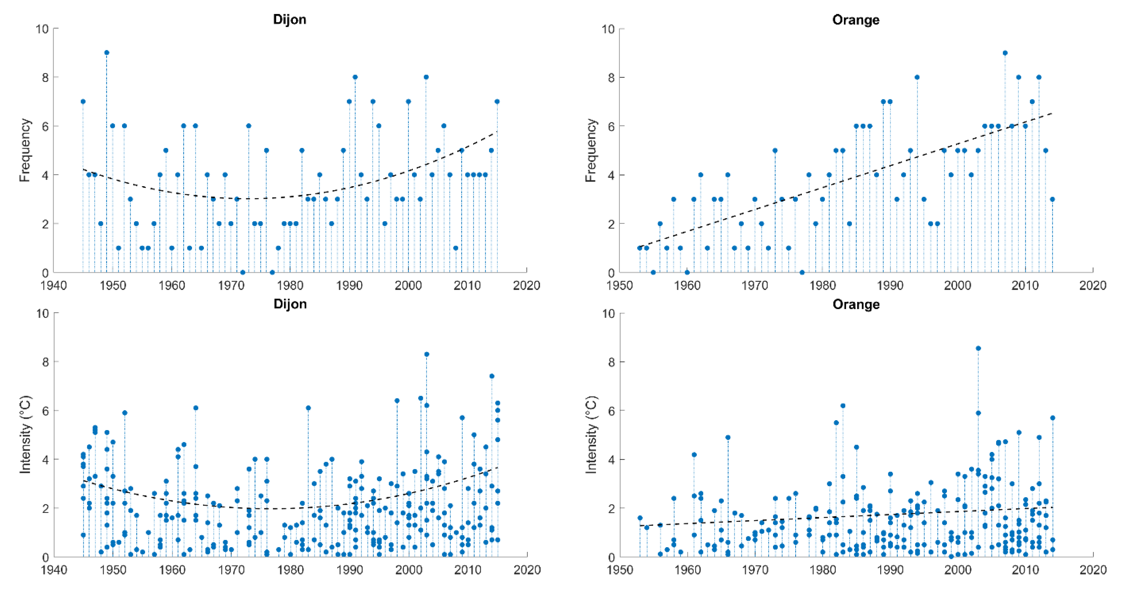
Identification and estimation of potential trends in heat spell characteristics are discussed in this subsection. The NS models with Time as a covariate were fitted to the time series. Trends in the model parameters λ t , σ t , and p t were analyzed as these parameters allow for the inference of trends in the frequency ( λ t ), intensity ( σ t ), and duration ( p t ) of heat spells. Figure 4 presents the time series with optimal trends in the time-dependent scale parameter of each distribution. Relationships for λ t , σ t , and p t , as used in the case of Orange, were of the form a 0 + a 1 t , and in the case of Dijon, had the form a 0 + a 1 t + a 2 t 2 . According to the likelihood ratio test [33,37], trends are significant at the 5% level for all the time series.
All the times series showed increasing trends from the 1970s to the present for Dijon. In Orange, constant increasing trends in all the time series were observed from the beginning of the time series. It is also interesting to note that the longest heat spell occurrd in Orange during the summer season of 2003 (about 25 days) and this event was also the most intense heat spell that occurred during the whole record period. It should be emphasized that the 2003 heat wave lasted only for 15 days in Dijon. The longest heat spell experienced by Dijon occurred during the summer of 1976, documented as the most severe drought period over the last few decades in France [65].

4.2.3. Correlations between CIs and Heat Spell Variables

As mentioned in the introductory section, the sub-decadal NAO, multidecadal AMO, and pacific-decadal PNA are three important CIs known to have an influence on summertime weather patterns in Europe and France. These CIs and Time are the four covariates used in the non-stationary case. The case of non-stationary distributions varying with these covariates were then considered and different combinations were used, allowing for quadratic relationships, as a maximum, to exist between a distribution parameter and covariate. Precise months can be used to compute the covariates NAO, AMO, and PNA. Here, a simple method was used, wherein the average for a 3-month period with different lags was obtained. The covariate Time is defined by integers incremented from 1 to the number of years in the series in the case of the frequency of heat spells. Time for the duration and intensity was considered fixed over the summer in each year but was allowed to shift from one year to the next.
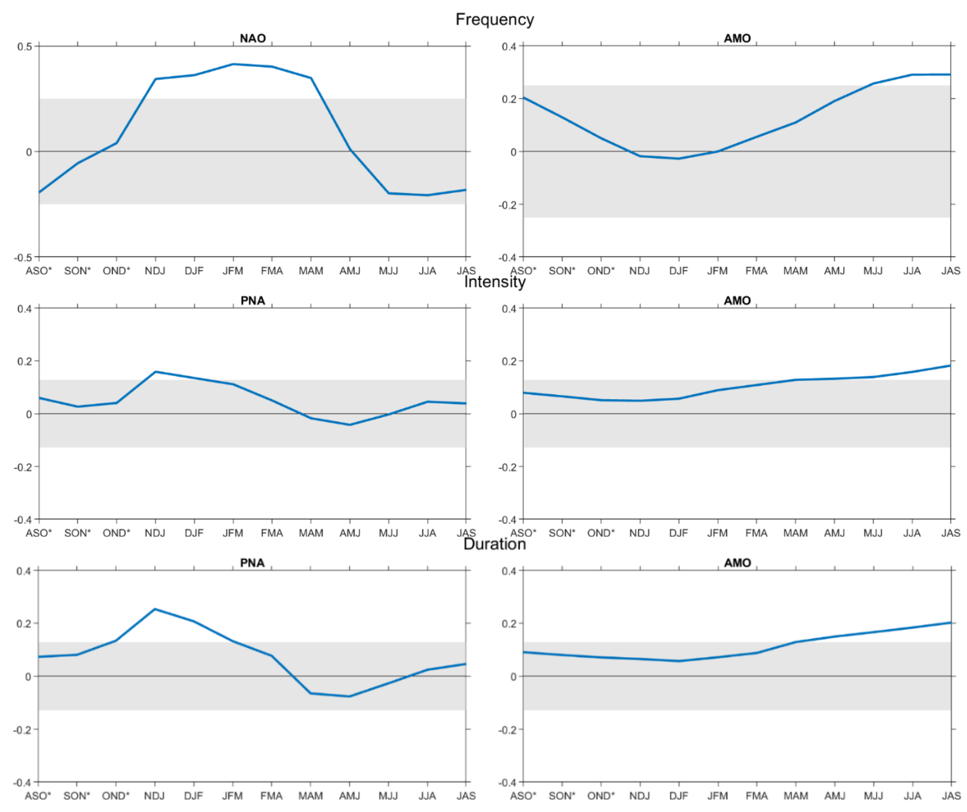
Relationships of seasonal CIs with the heat spell variables were evaluated by using correlations to select the optimal seasonal covariates. Figure 5 presents the temporal evolution of the Pearson correlation coefficients between the heat spell variables and the 3-month average of the selected CIs at Orange (the results for Dijon are very similar). The shaded area in the figures represents the limits where correlations were significant at a 5% level. Based on these results, the selected covariates were NAO(JFM) and AMO(JAS) for the frequency, as well as PNA(NDJ) and AMO(JAS) for the intensity and duration.
The correlation between the heat spell variables and the selected covariates Time, NAO(JFM), AMO(JAS), and PNA(NDJ) is presented in Table 1. Apart from the frequency of the heat spells at Orange, the correlations with Time are weak. NAO(JFM) is only correlated with the frequency of heat spells, while duration and intensity are systematically significantly correlated with both covariates PNA(NDJ) and AMO(JAS).

4.3. NS Frequency Analysis

The heat spell frequency, intensity, and duration were estimated with the NS- GP, POI, and GEO distribution functions. The NS- GP, POI, and GEO distributions were then applied to the time series of the heat spell characteristics. The period of 1950–2017, for which all the CIs are available, was used to conduct the NS frequency analysis. All the combinations of the selected covariates (single covariate, two covariates, and three covariates) were used to apply the NS models (presented in Section 2.2.1) on the time series of heat spell characteristics. The models, as presented in Table 2 and Table 3, represent the variation of the parameters of these distributions as a function of the covariates. Several models (up to the quadratic regression) were then proposed as functions of the covariates. The parameters of these regressions were also estimated with the maximum likelihood method. The stationary models were also tested in each case. Models with more parameters (quadratic relation rather than linear, for instance) were only selected if the AIC and BIC selected them despite the penalty they possess. We kept in mind that AIC and BIC penalize models with more parameters; it’s the principle of parsimony.
The optimal models were obtained according to the AIC for each possible configuration of the covariates. It is worth noting that the choices of the different probability functions (GP for intensity, POI for the frequency, and GEO for the duration) used to model heat spell variables were validated (not presented in this paper). It is then assumed here that the selected theoretical probability distributions are suitable to model the heat spell variables. Table 2 and Table 3 present the optimal model for each covariate configuration. The AIC and BIC statistics obtained for each optimal model and whose values were used to compare goodness-of-fits are also presented.
It can be observed here that for a given variable, the NS models with one or more covariates fit the observations systematically better than the stationary model according to AIC. For models including one covariate, the best fits in the case of Dijon were obtained with NAO for the frequency, Time for the intensity, and PNA for the duration. For Orange, the best fits were obtained with Time for the frequency and PNA for both the intensity and duration. It must be noted that multidecadal oscillations may generate temporal trends. However, in addition to multidecadal oscillations, a temporal trend was also statistically detected. This was confirmed by the selected models. Indeed, despite the adoption of the AIC and BIC criteria, which favor parsimonious models, models integrating both Time and Cis end revealed to be selected as optimal models. Overall best fits were generally obtained with two covariates. Indeed, for the Dijon case, the overall best fits were obtained with NAO and AMO for the frequency, Time and PNA for the intensity, and PNA and AMO for the duration. For Orange, overall best fits were obtained with PNA and AMO for both the intensity and duration, while for the frequency, it was the model with Time only.
The results also show that the inclusion of Time with CIs, Time and NAO, or Time and AMO, in both stations, enhanced the CI-varying model for the frequency. This result suggests that there is a strong temporal trend in the frequency that is not explained by the CIs. For the intensity, adding Time to AMO or PNA improved also the goodness-of-fit in Dijon but not in Orange. However, a larger impact on the goodness-of-fit with PNA and Time, rather than with AMO and Time, was observed. For the duration and in both stations, models that combined Time with the teleconnection patterns AMO or PNA resulted in underperformed models that included only these CIs. Additionally, it is interesting that both stations, including two CIs in any model for any variable, improved the goodness-of-fit compared to the models using each CI separately. This means that all the paired indices were somehow complementary and thus it is of interest to use them together. Using combinations of the three covariates Time, NAO, and AMO for frequency and Time, AMO, and PNA for both intensity and duration leads to weaker models. It can be concluded from these results that the variability in the heat spell variables is significantly explained by CIs. The temporal trend associated with global warming has an important impact on the frequency and intensity in Dijon, but a weaker impact on the duration.
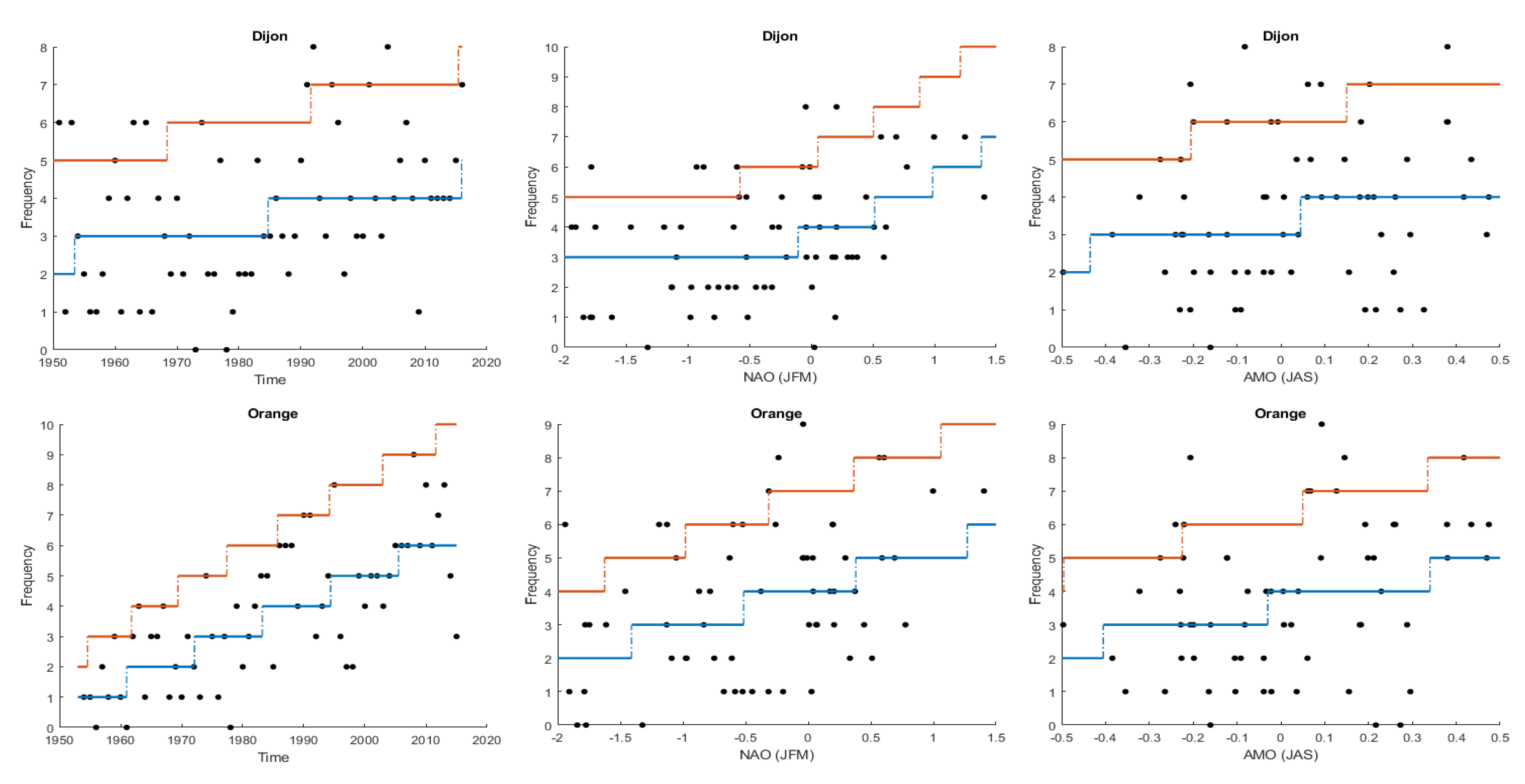
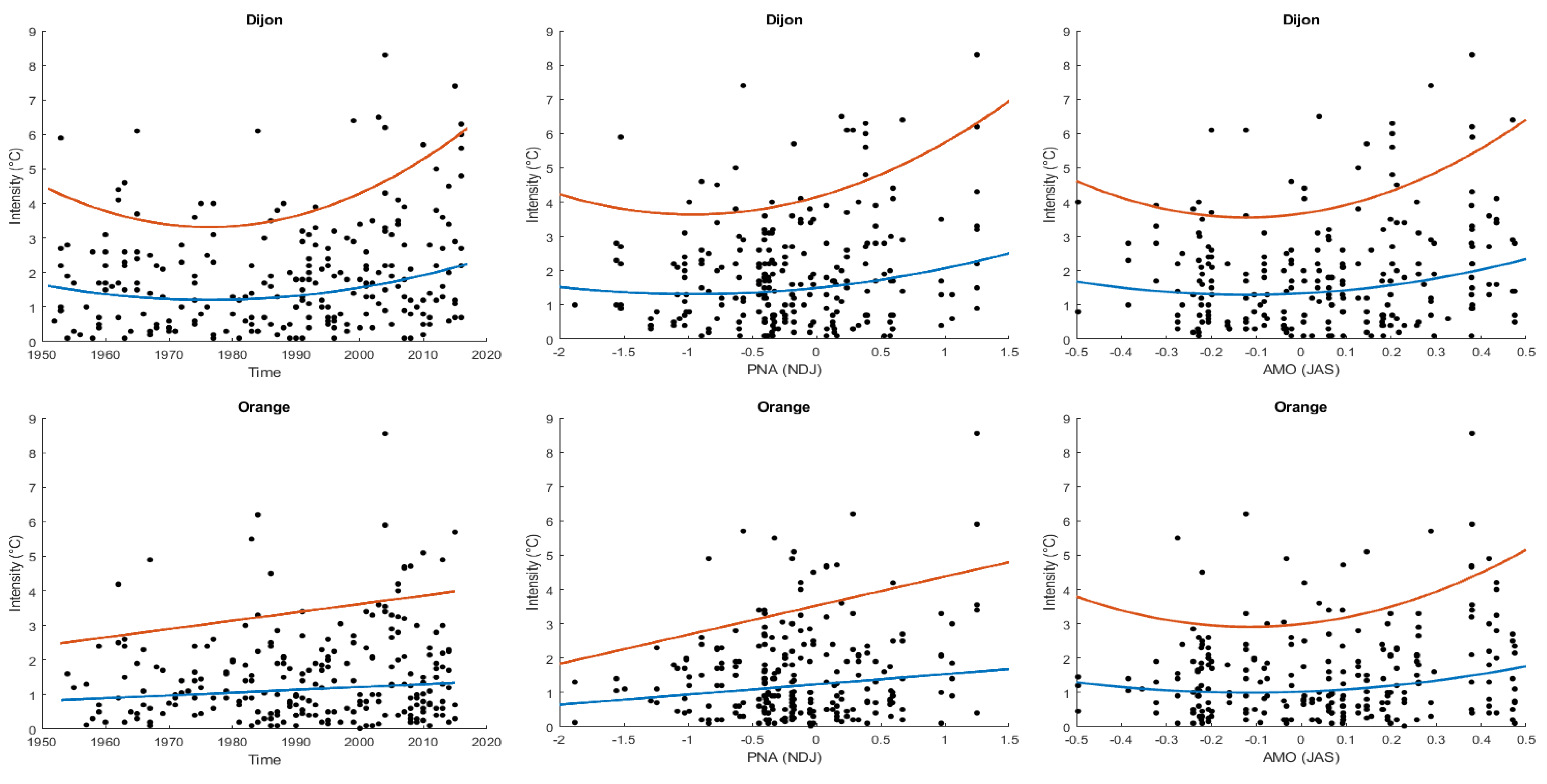
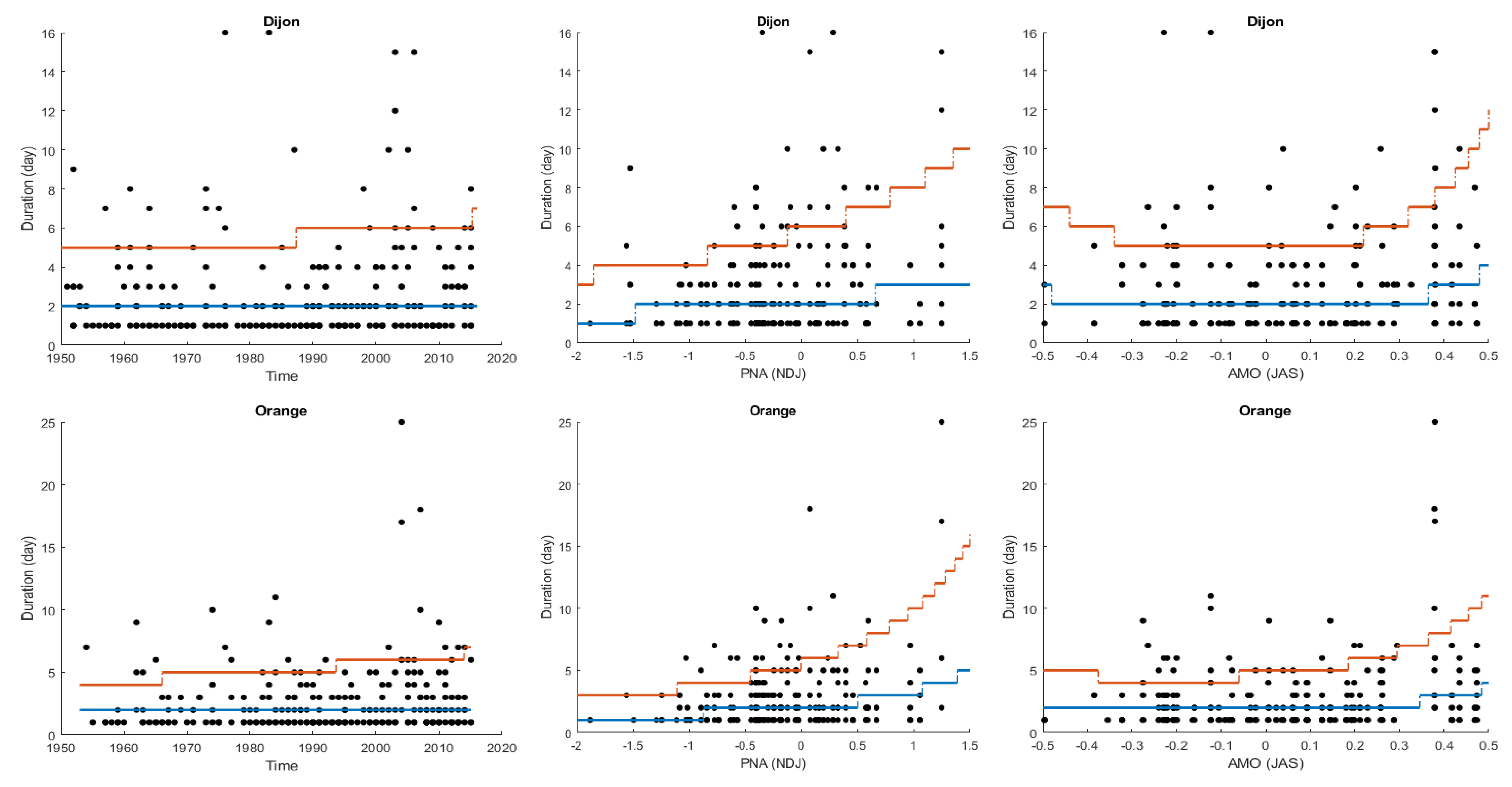
Other results related to the NS frequency analysis and more specifically to the quantiles corresponding to specific non-exceedance probabilities are presented in this section. The quantiles for the heat spell variables frequency, intensity, and duration, as obtained for probabilities p = 0.5 and p = 0.9 with the non-stationary models, including one covariate, are presented in Figure 6, Figure 7 and Figure 8, respectively. They are then presented as a function of the covariates Time, NAO, and AMO for the frequency, and Time, PNA, and AMO for both the intensity and duration. The quantiles corresponding to the variables frequency and duration are represented with step functions (vary constantly in sections), as the POI and GEO probability distributions are discrete. There are at least two aspects that can be analyzed in connection with these figures. First, it can be seen in Figure 7 and Figure 8 that for the intensity and duration, an important heat event that occurred in Orange during the summer of 2003 appears as an outlier and the values of PNA(NDJ) and AMO(JAS), as associated to this event, are in the extreme positive phase for both variables. Second, it can be seen in these figures (top and right panels in Figure 7 and right panel in Figure 8) that the relationships of the quantiles with the covariates are rather unrealistic in some cases (the intensity quantiles with Time, PNA, and AMO in Orange, and the intensity and duration quantiles with AMO for the two case studies) when the quadratic relationships are used. Indeed, quadratic models were selected in these cases, resulting in decreasing trends on the left side and increasing trends on the right side.
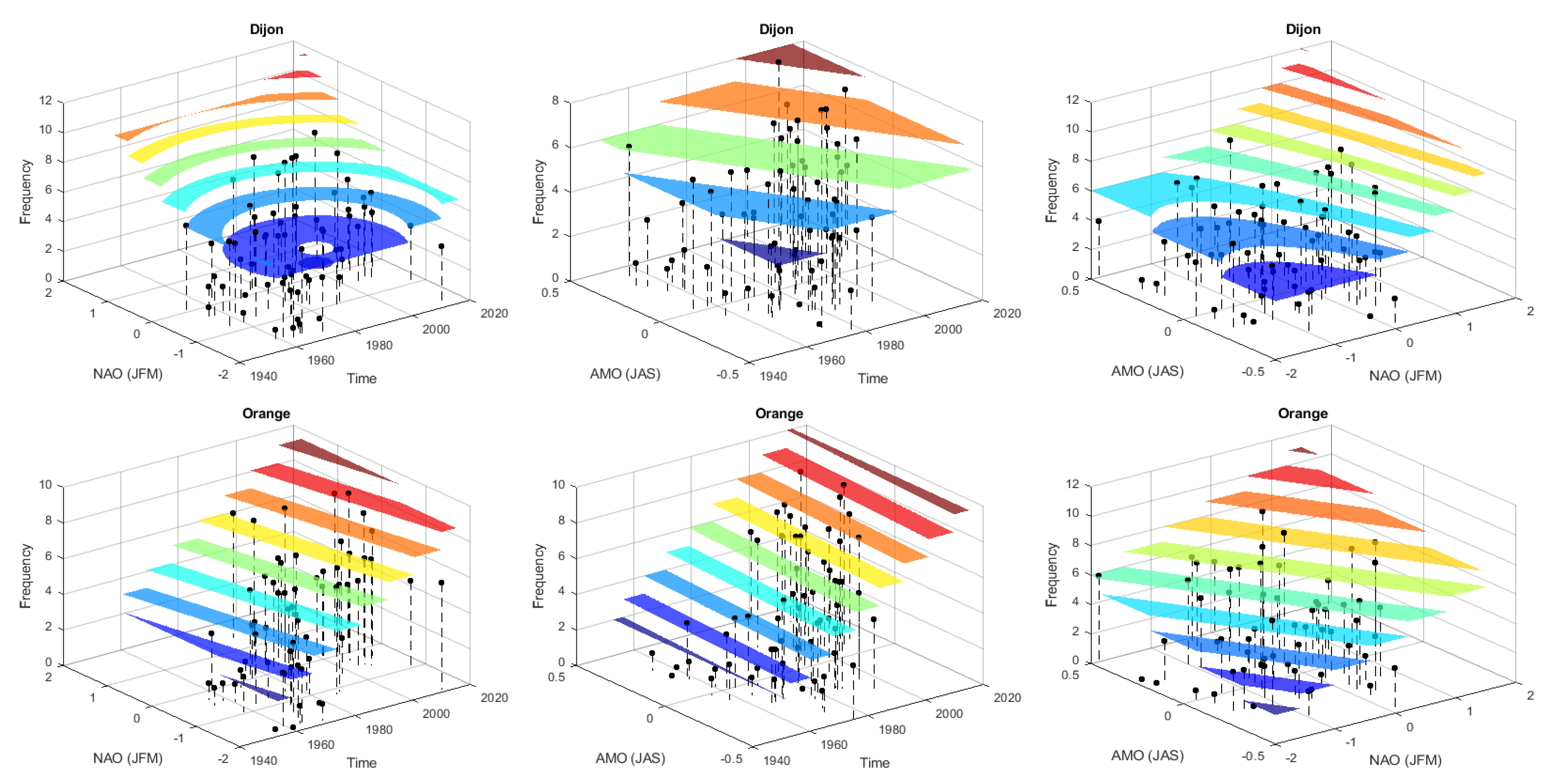
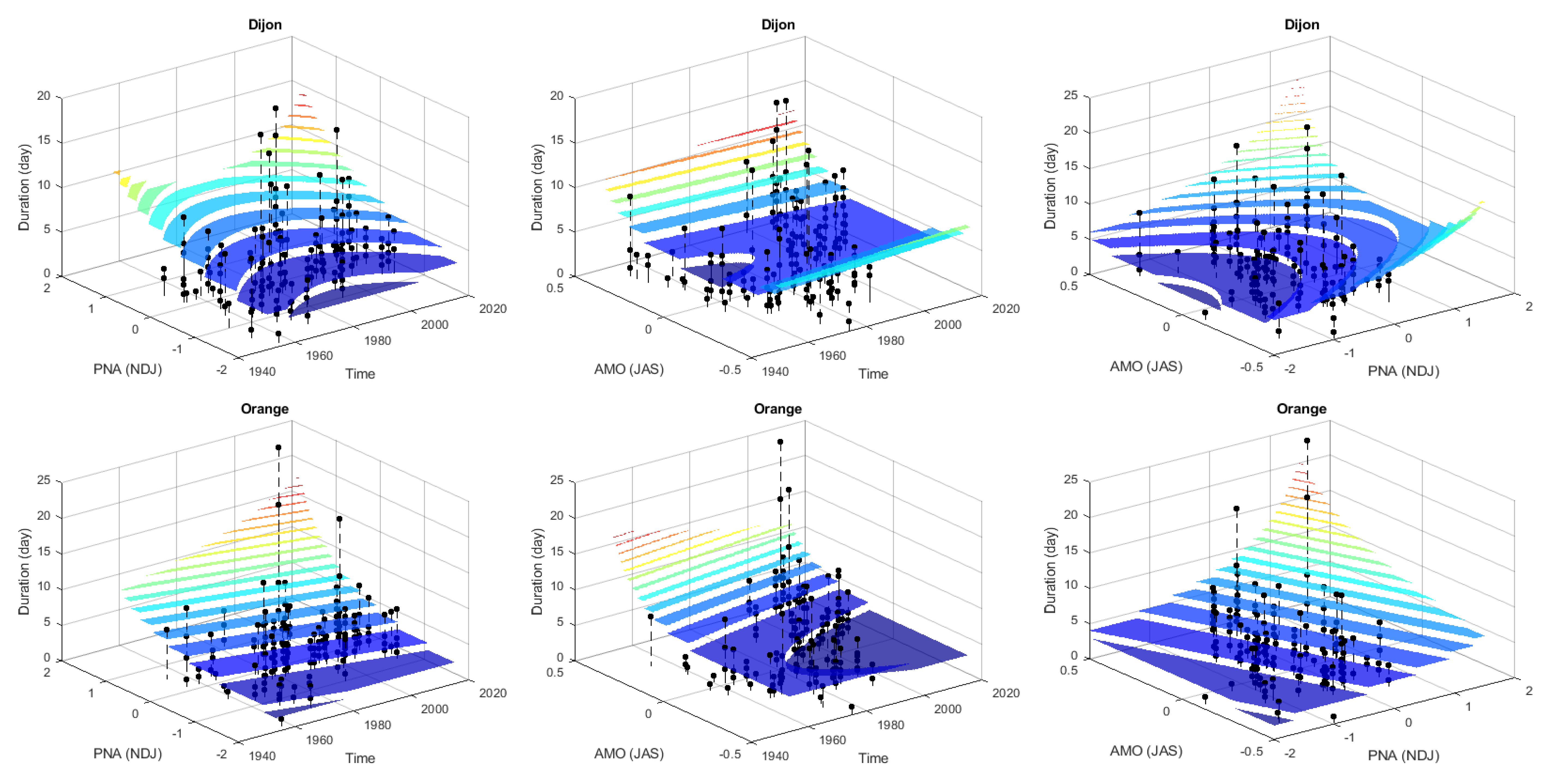
The quantiles corresponding to the non-exceedance probability p = 0.9 obtained with the non-stationary models including two covariates are presented in Figure 9, Figure 10 and Figure 11 for the frequency, duration, and intensity respectively. These figures show the optimal NS models combining all the pairs of the covariates in the form of three-dimensional graphs. As with the one-covariate NS model and for the same reasons, quantiles corresponding to the frequency and duration are also represented here with step functions. Such graphs allow the impact of each covariate in the NS models, with covariates on the heat spell characteristics, to be observed. For instance, one can easily observe the combined effect of the two climate indices, namely NAO and AMO, in the modeling frequency, and PNA and AMO in the modeling intensity and duration. Indeed, when both CIs have positive extreme values (or negative ones), the quantiles are extreme either very strong or very weak. A more thorough analysis may also show that increasing temporal trends are observed in the case of models combining Time with all covariates, which is intuitive in a context of global warming.
The objective of this work is to characterize heat spells at specific locations representative of two nuclear power plants in France. It was applied in the present work by using temperatures from central and southern France, more specifically in Dijon and Orange, respectively. However, future work will focus on the development of a regional model in which the geographical and physiographical characteristics (latitude, longitude, altitude, urbanization, land cover, percentage of forest, area covered by water, etc.) are integrated as covariates. The model will then be able to estimate heat spell parameters even in ungauged sites.
Additionally, Dijon (in central France) is 400 km away from Orange (southern France). The results show that large-scale patterns do not have the same influence on central and southern France. As indicated above, microclimates may exist and variables such as the altitude of the location can have significant impacts on heat spell signatures.

5. Conclusions

In this paper, heat spell events were identified from the time series of daily maximum temperatures during the summer season at two stations located in central and southern France. From these events, the heat spell frequency, duration, and intensity were extracted. It was shown in this paper that the heat spell characteristics in France are highly non-stationary: temporal trends were detected in the heat spell characteristics and relationships with large-scale teleconnection patterns characterized by climate indices were detected. Conditional distributions were used to account for the non-stationarities associated with global warming and climate oscillation patterns. Four covariates were included in the non-stationary modeling: Time, representing the temporal trend related to global warming, and three CIs, namely NAO, AMO, and PNA, that partly explain the variability of temperatures in France. It was shown that the goodness-of-fit of the NS models with one or more covariates is systematically better than that of the stationary model according to the AIC and BIC statistics. Additionally, overall best fits were generally obtained with combinations of two covariates.
From the results, conditions that can potentially lead to adverse heat-related impacts can be identified as follows:
Global warming may increase the likelihood of heat spell variables.
The impact on the frequency of the NAO index of the preceding winter is in its extreme positive phase.
The combined effect on the frequency in central France of the NAO index of the preceding winter and of the AMO in summer are both in their extreme positive phases.
The combined effect on the intensity and duration of the PNA index of the preceding winter and of the AMO index in summer are both in their extreme positive phase.
The use of covariates in a NS analysis is useful for making a more appropriate assessment of the risks related to extreme temperatures. Such an approach can find applications for periodic safety reviews during the lifetime of sensitive facilities such as nuclear power plants.
Future work should focus on the development of a regional model in which the geographical and physiographical characteristics of the site (latitude, longitude, altitude, land cover, percentage of forest, area covered by water, etc.) are integrated directly as covariates into the model. The objective is to develop models that are able to estimate heat spell parameters even in ungauged sites.

Author Contributions

Conceptualization, Y.H. and T.B.M.J.O.; methodology, T.B.M.J.O. and C.C.; validation, T.B.M.J.O., Y.H. and C.C.; formal analysis, T.B.M.J.O. and Y.H.; investigation, T.B.M.J.O., C.C. and Y.H.; data curation, Y.H.; writing—original draft preparation, Y.H.; writing—review and editing, C.C., Y.H. and T.B.M.J.O.; supervision, T.B.M.J.O. and Y.H.; project administration, T.B.M.J.O. and Y.H.; funding acquisition, T.B.M.J.O. All authors have read and agreed to the published version of the manuscript.

Funding

This research received no external funding.

Institutional Review Board Statement

Not applicable.

Informed Consent Statement

Not applicable.

Data Availability Statement

Datasets analyzed in this study are not publicly available.

Acknowledgments

The authors wish to thank Météo-France for supplying the temperature data used in this study.

Conflicts of Interest

The authors declare no conflict of interest.

References

  1. Cassou, C.; Terray, L.; Phillips, A.S. Tropical Atlantic influence on European heatwaves. J. Clim. 2005, 18, 2805–2811. [Google Scholar] [CrossRef]
  2. Jones, P.D.; Moberg, A. Hemispheric and large-scale surface air temperature variations: An extensive revision and an update to 2001. J. Clim. 2003, 16, 206–223. [Google Scholar] [CrossRef] [Green Version]
  3. Tank, A.M.G.K.; Können, G.P. Trends in indices of daily temperature and precipitation extremes in Europe, 1946–1999. J. Clim. 2003, 16, 3665–3680. [Google Scholar] [CrossRef]
  4. Beniston, M. The 2003 heat wave in Europe: A shape of things to come? An analysis based on Swiss climatological data and model simulations. Geophys. Res. Let. 2004, 31, 384. [Google Scholar] [CrossRef] [Green Version]
  5. Schär, C.; Vidale, P.L.; Lüthi, D.; Frei, C.; Häberli, C.; Liniger, M.A.; Appenzeller, C. The role of increasing temperature variability in European summer heatwaves. Nature 2004, 427, 333–336. [Google Scholar] [CrossRef]
  6. Poumadere, M.; Mays, C.; Mer, S.L.; Blong, R.J. The 2003 heat wave in France: Dangerous climate change here and now. Risk Anal. 2005, 25, 1483–1494. [Google Scholar] [CrossRef]
  7. Fouillet, A.; Ray, G.; Laurent, F.; Bellec, S.; Guihenneuc-Jouyaux, C.; Clavel, J.; Jougla, E.; Hémon, D. Excess mortality related to the August 2003 heat wave in France. Int. Arch. Occup. Environ. Health 2006, 80, 16–24. [Google Scholar] [CrossRef] [Green Version]
  8. Alexander, L.V.; Zhang, X.; Peterson, T.C.; Caesar, J.; Gleason, B.; Tank, A.M.G.K.; Haylock, M.; Collins, D.; Trewin, B.; Rahimzadeh, F.; et al. Global observed changes in daily climate extremes of temperature and precipitation. J. Geophys. Res. Atmos. 2006, 111. [Google Scholar] [CrossRef] [Green Version]
  9. Brown, S.J.; Caesar, J.; Ferro, C.A.T. Global changes in extreme daily temperature since 1950. J. Geophys. Res. Atmos. 2008, 13. [Google Scholar] [CrossRef] [Green Version]
  10. Coumou, D.; Rahmstorf, S. A decade of weather extremes. Nat. Clim. Change 2012, 2, 491–496. [Google Scholar] [CrossRef]
  11. Coumou, D.; Robinson, A. Historic and future increase in the global land area affected by monthly heat extremes. Environ. Res. Lett. 2013, 8, 034018. [Google Scholar] [CrossRef]
  12. Parey, S.; Malek, F.; Laurent, C.; Dacunha-Castelle, D. Trends and climate evolution: Statistical approach for very high temperatures in France. Clim Change. 2007, 81, 331–352. [Google Scholar] [CrossRef] [Green Version]
  13. Hansen, J.; Ruedy, R.; Sato, M.; Lo, K. Global surface temperature change. Rev. Geophys. 2010, 48. [Google Scholar] [CrossRef] [Green Version]
  14. Basha, G.; Kishore, P.; Ratnam, M.V.; Jayaraman, A.; Agha Kouchak, A.; Ouarda, T.B.M.J.; Velicogna, I. Historical and Projected Surface Temperature over India during the 20th and 21st century. Sci. Rep. 2017, 7, 2987. [Google Scholar] [CrossRef] [PubMed] [Green Version]
  15. IPCC. Managing the Risks of Extreme Events and Disasters to Advance Climate Change Adaptation. A Special Report of Working Groups I and II of the Intergovernmental Panel on Climate Change; IPCC: Geneva, Switzerland, 2012; p. 582. [Google Scholar]
  16. Ouarda, T.B.M.J.; Charron, C.; Kumar, K.N.; Phanikumar, D.V.; Molini, A.; Basha, G. Nonstationary warm spell frequency analysis integrating climate variability and change with application to the Middle East. Clim. Dyn. 2019, 53, 5329–5347. [Google Scholar] [CrossRef]
  17. Ouzeau, G.; Soubeyroux, J.M.; Schneider, M.; Vautard, R.; Planton, S. Heat waves analysis over France in present andfuture climate: Application of a new method on the EURO-CORDEX ensemble. Clim. Serv. 2016, 4, 1–12. [Google Scholar] [CrossRef] [Green Version]
  18. Pausader, M.; Bernie, D.; Parey, S.; Nogaj, M. Computing the distribution of return levels of extreme warm temperatures for future climate projections. Clim. Dyn. 2012, 38, 1003–1015. [Google Scholar] [CrossRef]
  19. Ouzeau, G.; Déqué, M.; Jouini, M.; Planton, S.; Vautard, R. Le Climat de la France au XXIe Siècle Volume 4-Scénarios Régionalisés: Édition 2014 Pour la Métropole et les Régions D’outre-mer. 2014. Available online: https://www.actu-environnement.com/media/pdf/news-22612-onerc-climat-france.pdf (accessed on 15 February 2021).
  20. Milenković, M.; Ducić, V.; Burić, D.; Lazić, B. The Atlantic Multidecadal Oscillation (AMO) and the forest fires in France in the period 1980–2014. J. Geogr. Inst. Jovan Cvijic SASA 2016, 66, 35–44. [Google Scholar] [CrossRef]
  21. Giuntoli, B.; Renard, J.P.; Vidal, A.B. Low Flows in France and their relationship to large scale climate indices. J. Hydrol. 2013, 482, 105–118. [Google Scholar] [CrossRef] [Green Version]
  22. Barnston, A.G.; Livezey, R.E. Classification, seasonality and persistence of low-frequency atmospheric circulation patterns. Mon. Wea. Rev. 1987, 115, 1083–1126. [Google Scholar] [CrossRef]
  23. Wallace, J.M.; Gutzler, D.S. Teleconnections in the geopotential height field duringthe Northern Hemisphere winter. Mon. Weather. Rev. 1981, 109, 784–812. [Google Scholar] [CrossRef]
  24. Cattiaux, J. Extrêmes de Température en Europe: Mécanismes et Réponses au Changement Climatique. Ph.D. Thesis, Pierre et Marie Curie University, Paris, France, 2010. [Google Scholar]
  25. Conte, M.; Giuffrida, S.; Tedesco, S. The Mediterranean oscillation: Impact on precipitation and hydrology in Italy. Dans Clim. Water 1989, 121–137. [Google Scholar]
  26. Efthymiadis, D.; Goodess, C.M.; Jones, P.D. Trends in Mediterranean gridded temperature extremes and large-scale circulation influences. Nat. Hazards Earth Syst. Sci. 2011, 11, 2199–2214. [Google Scholar] [CrossRef]
  27. Ouachani, R.; Bargaoui, Z.; Ouarda, T.B.M.J. Power of teleconnection patterns on precipitation and streamflow variability of upper Medjerda Basin. Int. J. Climatol. 2013, 33, 58–76. [Google Scholar] [CrossRef]
  28. Naizghi, M.S.; Ouarda, T.B.M.J. Teleconnections and analysis of long-term wind speed variability in the UAE. Int. J. Climatol. 2017, 37, 230–248. [Google Scholar] [CrossRef]
  29. Ouarda, T.B.M.J.; Charron, C.; St-Hilaire, A. Uncertainty of stationary and nonstationary models for rainfall frequency analysis. Int. J. Climatol. 2020, 40, 2373–2392. [Google Scholar] [CrossRef]
  30. Keellings, D.; Waylen, P. Investigating teleconnection drivers of bivariate heat waves in Florida using extreme value analysis. Clim. Dyn. 2015, 44, 3383–3391. [Google Scholar] [CrossRef]
  31. Khaliq, M.N.; Ouarada, T.; Gachon, P.; Sushama, L. Stochastic modeling of hot weather spells and their characteristics. Clim. Res. 2011, 47, 187–199. [Google Scholar] [CrossRef] [Green Version]
  32. Caroni, C.; Panagoulia, D. Non-stationary modelling of extreme temperatures in a mountainous area of Greece. REVSTAT 2016, 14, 217–228. [Google Scholar]
  33. Hamdi, Y.; Duluc, C.-M.; Rebour, V. Temperature Extremes: Estimation of Non-Stationary Return Levels and Associated Uncertainties. Atmosphere 2018, 9, 129. [Google Scholar] [CrossRef] [Green Version]
  34. Ouarda, T.B.M.J.; El-Adlouni, S. Bayesian nonstationary frequency analysis of hydrological variables. J. Am. Water Resour. Assoc. 2011, 47, 496–505. [Google Scholar] [CrossRef]
  35. Hundecha, Y.; St-Hilaire, A.; Ouarda, T.B.M.J.; El Adlouni, S.; Gachon, P. A nonstationary extreme value analysis for the assessment of changes in extreme annual wind speed over the gulf of St. Lawrence, Canada. J. Appl. Meteorol. Climatol. 2008, 47, 2745–2759. [Google Scholar] [CrossRef]
  36. Katz, R.W.; Parlange, M.B.; Naveau, P. Statistics of extremes in hydrology. Adv. Water. Resour. 2002, 25, 1287–1304. [Google Scholar] [CrossRef] [Green Version]
  37. Coles, S. An Introduction to Statistical Modeling of Extreme Values; Springer: New York, NY, USA, 2001. [Google Scholar]
  38. Hamdi, Y.; Bardet, L.; Duluc, C.-M.; Rebour, V. Extreme storm surges: A comparative study of frequency analysis approaches. Nat. Hazards Earth Syst. Sci. 2014, 14, 2053–2067. [Google Scholar] [CrossRef] [Green Version]
  39. Pickands, J. Statistical inference using extreme order statistics. Ann. Stat. 1975, 3, 119–131. [Google Scholar]
  40. Ashkar, F.; Ouarda, T.B.M.J. On some methods of ftting the generalized Pareto distribution. J. Hydrol. 1996, 177, 117–141. [Google Scholar] [CrossRef]
  41. Whitaker, L. On the Poisson law of small numbers. Biometrika 1914, 10, 36–71. [Google Scholar] [CrossRef]
  42. Furrer, E.; Katz, R.W.; Walter, M.D.; Furrer, R. Statistical modeling of hot spells and heat waves. Clim. Res. 2010, 43, 191–205. [Google Scholar] [CrossRef] [Green Version]
  43. Keellings, D.; Waylen, P. Increased risk of heat waves in Florida: Characterizing changes in bivariate heat wave risk using extreme value analysis. Appl. Geogr. 2014, 46, 90–97. [Google Scholar] [CrossRef]
  44. Wang, W.; Zhou, W.; Li, Y.; Wang, X.; Wang, D. Statistical modeling and CMIP5 simulations of hot spell changes in China. Clim. Dyn. 2015, 44, 2859–2872. [Google Scholar] [CrossRef]
  45. Beguería, S.; Angulo-Martínez, M.; Vicente-Serrano, S.M.; López-Moreno, J.I.; El-Kenawy, A. Assessing trends in extreme precipitation events intensity and magnitude using non-stationary peaks-over-threshold analysis: A case study in northeast Spain from 1930 to 2006. Int. J. Climatol. 2011, 31, 2102–2114. [Google Scholar] [CrossRef] [Green Version]
  46. Panagoulia, D.; Economou, P.; Caroni, C. Stationary and nonstationary generalized extreme value modelling of extreme precipitation over a mountainous area under climate change. Environmetrics 2014, 25, 29–43. [Google Scholar] [CrossRef]
  47. Ouarda, T.B.M.J.; Charron, C. Changes in the distribution of hydro-climatic extremes in a non-stationary framework. Sci. Rep. 2019, 9, 8104. [Google Scholar] [CrossRef] [PubMed] [Green Version]
  48. Ouarda, T.B.M.J.; Charron, C. Non-stationary statistical modelling of wind speed: A case study in eastern Canada. Energy Convers. Manag. 2021, 236, 114028. [Google Scholar] [CrossRef]
  49. Robinson Peter, J. On the Definition of a Heat Wave. J. App. Meteor. 2001, 40, 762–775. [Google Scholar] [CrossRef]
  50. Russo, S.; Dosio, A.; Graversen, R.G.; Sillmann, J.; Carrao, H.; Dunbar, M.B.; Singleton, A.; Montagna, P.; Barbola, P.; Vogt, J.V. Magnitude of extreme heat waves in present climate and their projectionin a warming world. J. Geophys. Res.-Atmos. 2014, 119, 12500–12512. [Google Scholar] [CrossRef] [Green Version]
  51. Frich, P.; Alexander, L.V.; Della-Marta, P.; Gleason, B.; Haylock, M.; Klein Tank, A.; Peterson, T. Global changes in climatic extremes during the 2nd half of the 20th century. Clim. Res. 2002, 19, 193–212. [Google Scholar] [CrossRef] [Green Version]
  52. Rafferty, J.P. Heat Wave. 5 December 2018. Available online: https://www.britannica.com/science/heat-wave-meteorology (accessed on 23 May 2021).
  53. Perkins, S.E.; Alexander, L.V. On the measurement of heat waves. J. Clim. 2012, 26, 4500–4517. [Google Scholar] [CrossRef]
  54. Della-Marta, P.M.; Haylock, M.R.; Luterbacher, J.; Wanner, H. Doubled length of western European summer heat waves since 1880. J. Geophys. Res.-Atmos. 2007, 112. [Google Scholar] [CrossRef] [Green Version]
  55. Stefanon, M.; Fabio, D.; Drobinski, P. Heatwave classification over Europe and the Mediterranean region. Environ. Res. Lett. 2012, 7, 014023. [Google Scholar] [CrossRef]
  56. Bladé, I.; Fortuny, D.; Van Oldenborgh, G.J.; Liebmann, B. The summer North Atlantic Oscillation in CMIP3 models and related uncertainties in projected summer drying in Europe. J. Geophys. Res.-Atmos. 2012, 117. [Google Scholar] [CrossRef] [Green Version]
  57. Folland, C.K.; Knight, J.; Linderholm, H.W.; Fereday, D.; Ineson, S.; Hurrell, J.W. The Summer North Atlantic Oscillation: Past, Present, and Future. J. Clim. 2009, 22, 1082–1103. [Google Scholar] [CrossRef]
  58. Fuentes-Franco, R.; Koenigk, T. Identifying remote sources of interannual variability for summer precipitation over Nordic European countries tied to global teleconnection wave patterns. Dyn. Meteorol. Oceanogr. 2020, 72, 1–15. [Google Scholar] [CrossRef]
  59. Kingston, D.G.; McGregor, G.R.; Hannah, D.M.; Lawler, D.M. River flow teleconnections across the northern North Atlantic region. Geophys. Res. Lett. 2006, 33. [Google Scholar] [CrossRef]
  60. Knight, J.R.; Folland, C.K.; Scaife, A.A. Climate impacts of the Atlantic Multidecadal Oscillation. Geophys. Res. Lett. 2006, 33. [Google Scholar] [CrossRef] [Green Version]
  61. Lamb, P.; Peppler, R. North Atlantic oscillation: Concept and an application. Bull. Amer. Meteor. Soc. 1987, 68, 1218–1225. [Google Scholar] [CrossRef]
  62. Wanner, H.; Brönnimann, S.; Casty, C.; Gyalistras, D.; Luterbacher, J.; Schmutz, C.; Stephenson, D.B.; Xoplaki, E. North Atlantic Oscillation–Concepts And Studies. Surv. Geophys. 2001, 22, 321–381. [Google Scholar] [CrossRef]
  63. Seidou, O.; Asselin, J.J.; Ouarda, T.B.M.J. Bayesian multivariate linear regression with application to change point models in hydrometeorological variables. Water. Resour. Res. 2007, 43. [Google Scholar] [CrossRef] [Green Version]
  64. Seidou, O.; Ouarda, T.B.M.J. Recursion-based multiple changepoint detection in multiple linear regression and application to river streamflows. Water. Resour. Res. 2007, 43. [Google Scholar] [CrossRef] [Green Version]
  65. Green, J.S.A. The weather during July I976: Some dynamical considerations of the drought. Weather 1977, 32, 120–126. [Google Scholar] [CrossRef]
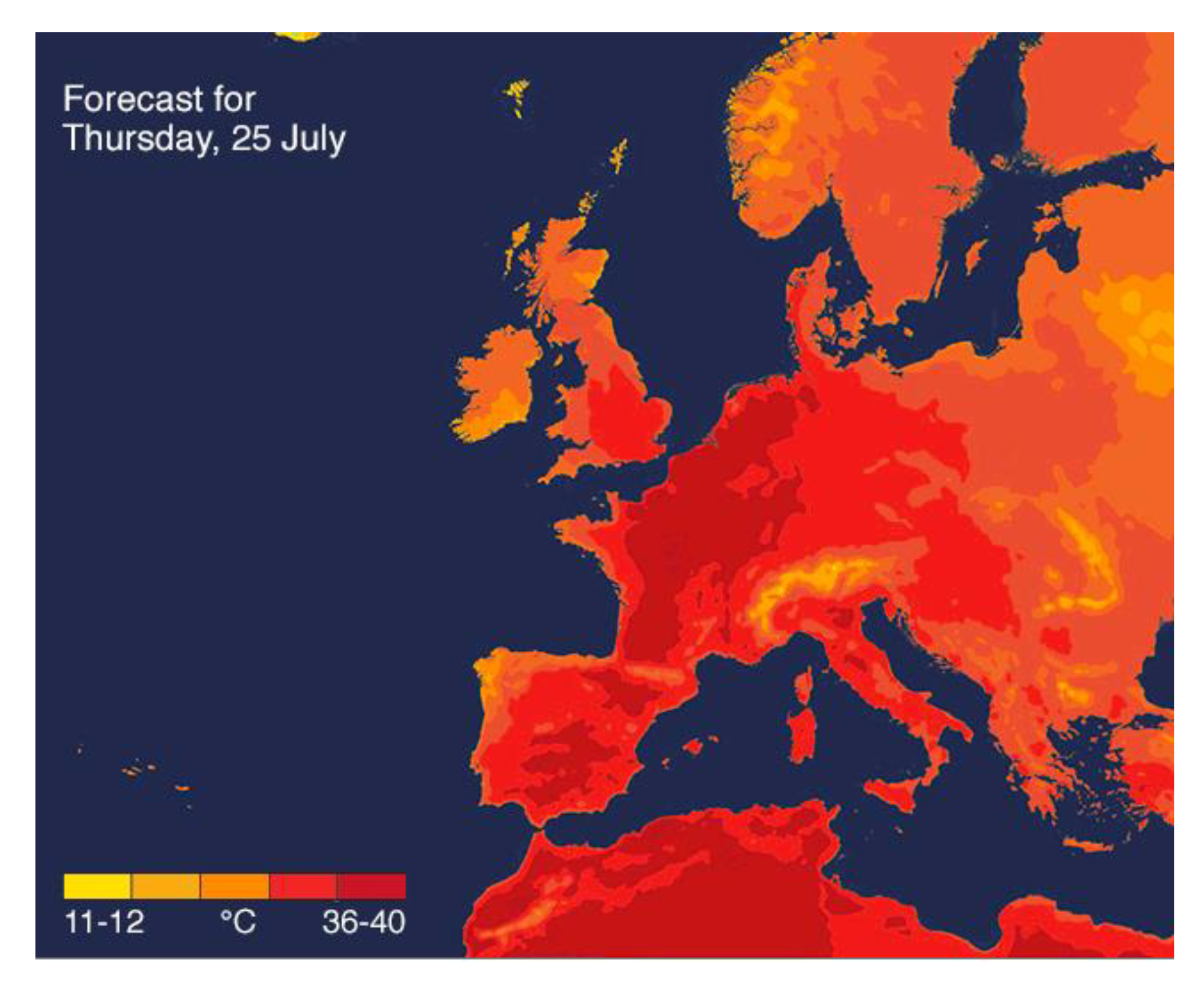
Figure 1. Record temperatures across Europe (forecast for 25 July 2019, source: BBC Weather).
Atmosphere 12 01387 g001
Figure 2. Case study (Orange and Dijon Stations): location map.
Atmosphere 12 01387 g002
Figure 3. Daily maximum temperature (light line) and threshold of the 90th percentile of the maximum temperature (Bold line) for the years 2002 and 2003 in Orange. Extreme heat events are identified by the gray areas.
Atmosphere 12 01387 g003
Figure 4. Time series for the heat spell frequency, intensity, and duration for both stations. The dashed line denotes the trend in the time-dependent distribution scale parameters ( λ t for the frequency, σ t for the intensity, and p t for the duration).
Atmosphere 12 01387 g004aAtmosphere 12 01387 g004b
Figure 5. Seasonal temporal evolution of the correlation coefficient between the heat spell variables in Orange and the selected climate indices. * denotes a season before the current year of the observed heat spells. The shaded area represents the limits where correlations are significant at a 5% level.
Atmosphere 12 01387 g005
Figure 6. Frequency quantiles corresponding to the non-exceedance probabilities p = 0.5 (blue line) and 0.9 (red line) as a function of each covariate.
Atmosphere 12 01387 g006
Figure 7. Intensity quantiles corresponding to the non-exceedance probabilities p = 0.5 (blue line) and 0.9 (red line) as a function of each covariate.
Atmosphere 12 01387 g007
Figure 8. Duration quantiles corresponding to the non-exceedance probabilities p = 0.5 (blue line) and 0.9 (red line) as a function of each covariate.
Atmosphere 12 01387 g008
Figure 9. Frequency quantiles corresponding to the non-exceedance probability p = 0.9 as a function of the combination of two covariates.
Atmosphere 12 01387 g009
Figure 10. Intensity quantiles corresponding to the non-exceedance probability p = 0.9 as a function of the combination of two covariates.
Atmosphere 12 01387 g010
Figure 11. Duration quantiles corresponding to the non-exceedance probability p = 0.9 as a function of the combination of two covariates.
Atmosphere 12 01387 g011
Table 1. Correlation coefficients between the heat spell variables and covariates.
StationVariableCovariate
TimeNAO (JFM)PNA (NDJ)AMO (JAS)
DijonFrequency0.190.41 *0.050.23 *
Duration0.040.110.18 *0.17 *
Intensity0.030.030.18 *0.15 *
OrangeFrequency0.71 *0.41 *0.150.29 *
Duration0.13<0.010.16 *0.18 *
Intensity0.10−0.030.25 *0.20 *
Note: Significant correlations at p < 5% are with *.
Table 2. The Dijon station corresponds to stationary/non-stationary models for each heat spell variable. AIC and BIC statistics for the optimal model of each configuration of covariates. For non-stationary models, different combinations of covariates were considered. In each case, the optimal non-stationary model based on the AIC statistic is presented.
VariableCovariate(s)AICBICModel
FrequencyStationary275.7277.9 POI ( λ t = 3.64 )
Time270.4274.8 POI ( λ t = 2.57 + 0.03 t )
NAO266.9273.4 * POI ( λ t = 3.82 + 1.42 NAO t + 0.47 NAO t 2 )
AMO273.8278.1 POI ( λ t = 3.59 + 2.08 AMO t )
Time + NAO267.1278.0 POI ( λ t = 4.03 0.06 t + 0.00 t 2 + 1.29 NAO t + 0.46 NAO t 2 )
Time + AMO270.9277.4 POI ( λ t = 2.65 + 0.03 t + 1.35 AMO t )
NAO + AMO265.1 *273.9 POI ( λ t = 3.77 + 1.42 NAO t + 0.47 NAO t 2 + 1.92 AMO t )
Time + NAO + AMO266.7275.5 POI ( λ t = 3.53 + 0.01 t + 0.77 NAO t + 1.67 AMO t )
Intensity
(°C)
Stationary765.7772.7 GP ( σ t = 2.32 , κ = 0.29 )
Time755.5769.3 GP ( σ t = 2.54 0.05 t + 0.00 t 2 , κ = 0.25 )
PNA759.8773.6 GP ( σ t = 2.34 + 0.59 PNA t + 0.31 PNA t 2 , κ = 0.24 )
AMO758.5772.3 GP ( σ t = 2.11 + 1.03 AMO t + 4.25 AMO t 2 , κ = 0.26 )
Time + PNA746.8 *767.6 * GP ( σ t = 3.15 0.07 t + 0.00 t 2 + 0.81 PNA t + 0.40 PNA t 2 , κ = 0.35 )
Time + AMO754.4775.1 GP ( σ t = 2.38 0.06 t + 0.00 t 2 0.71 AMO t + 5.15 PNA t 2 , κ = 0.25 )
PNA + AMO753.2770.4 GP ( σ t = 2.33 + 0.51 PNA t + 1.10 AMO t + 4.31 AMO t 2 , κ = 0.31 )
Time + PNA + AMO757.4774.7 GP ( σ t = 2.27 + 0.01 t + 0.31 PNA t + 0.89 AMO t ) , κ = 0.29 )
Duration
(Days)
Stationary840.6844.1 GEO ( p t = 0.37 )
Time839.5846.4 GEO ( p t = 0.44 0.00 t )
PNA831.4838.3 * GEO ( p t = 0.36 0.10 PNA t )
AMO832.2842.6 GEO ( p t = 0.43 0.09 AMO t 0.76 AMO t 2 )
Time + PNA832.6846.4 GEO ( p t = 0.31 + 0.01 t 0.00 t 2 0.09 PNA t )
Time + AMO833.9847.8 GEO ( p t = 0.45 0.00 t 0.08 AMO t 0.75 AMO t 2 )
PNA + AMO828.0 *841.9 GEO ( p t = 0.41 0.07 PNA t 0.05 AMO t 0.68 AMO t 2 )
Time + PNA + AMO832.0845.9 GEO ( p t = 0.38 0.00 t 0.08 PNA t 0.15 AMO t )
Note: Overall best AIC and BIC values are with *.
Table 3. The Orange station corresponds to stationary/non-stationary models for each heat spell variable. AIC and BIC statistics for the optimal model of each configuration of covariates. For non-stationary models, different combinations of covariates were considered. In each case, the optimal model based on the AIC statistic is presented.
VariableCovariate(s)AICBICModel
FrequencyStationary277.5279.7 POI ( λ t = 3.79 )
Time235.4 *239.7 * POI ( λ t = 0.96 + 0.09 t )
NAO265.6269.9 POI ( λ t = 4.25 + 1.12 NAO t )
AMO273.0277.3 POI ( λ t = 3.76 + 2.68 AMO t )
Time + NAO236.5242.9 POI ( λ t = 1.30 + 0.08 t + 0.30 NAO t )
Time + AMO237.3243.7 POI ( λ t = 0.95 + 0.09 t 0.31 AMO t )
NAO + AMO260.5266.9 POI ( λ t = 4.23 + 1.14 NAO t + 2.66 AMO t )
Time + NAO + AMO238.5247.0 POI ( λ t = 1.28 + 0.08 t + 0.29 NAO t 0.18 AMO t )
Intensity
(°C)
Stationary670.0676.9 GP ( σ t = 1.71 , κ = 0.20 )
Time667.7678.1 GP ( σ t = 1.27 + 0.01 t , κ = 0.14 )
PNA663.9674.2 * GP ( σ t = 1.90 + 0.46 PNA t , κ = 0.20 )
AMO664.3678.1 GP ( σ t = 1.56 + 0.71 AMO t + 3.09 AMO t 2 , κ = 0.16 )
Time + PNA664.1678.0 GP ( σ t = 1.59 + 0.01 t + 0.37 PNA t , κ = 0.19 )
Time + AMO666.3683.6 GP ( σ t = 1.53 + 0.00 t + 0.69 AMO t + 3.05 AMO t 2 , κ = 0.16 )
PNA + AMO662.8 *676.7 GP ( σ t = 1.85 + 0.34 PNA t + 0.69 AMO t , κ = 0.20 )
Time + PNA + AMO664.7682.0 GP ( σ t = 1.76 + 0.00 t + 0.33 PNA t + 0.60 AMO t , κ = 0.20 )
Duration
(Days)
Stationary840.8844.2 GEO ( p t = 0.37 )
Time838.6845.5 GEO ( p t = 0.47 0.00 t )
PNA818.8825.7 * GEO ( p t = 0.37 0.15 PNA t )
AMO826.6837.0 GEO ( p t = 0.43 0.22 AMO t 0.50 AMO t 2 )
Time + PNA819.0829.4 GEO ( p t = 0.44 0.00 t 0.14 PNA t )
Time + AMO828.2842.0 GEO ( p t = 0.39 + 0.00 t 0.26 AMO t 0.51 AMO t 2 )
PNA + AMO815.5 *825.9 GEO ( p t = 0.39 0.12 PNA t 0.19 AMO t )
Time + PNA + AMO817.5831.3 GEO ( p t = 0.38 + 0.00 t 0.12 PNA t 0.20 AMO t )
Note: Overall best AIC and BIC values are with *.
Publisher’s Note: MDPI stays neutral with regard to jurisdictional claims in published maps and institutional affiliations.