
Projected Changes in the Atmospheric Dynamics of Climate Extremes in France


Abstract
1. Introduction
2. Data
2.1. Observations and Reanalyses
2.2. Climate Model Simulations
3. Selection of Events
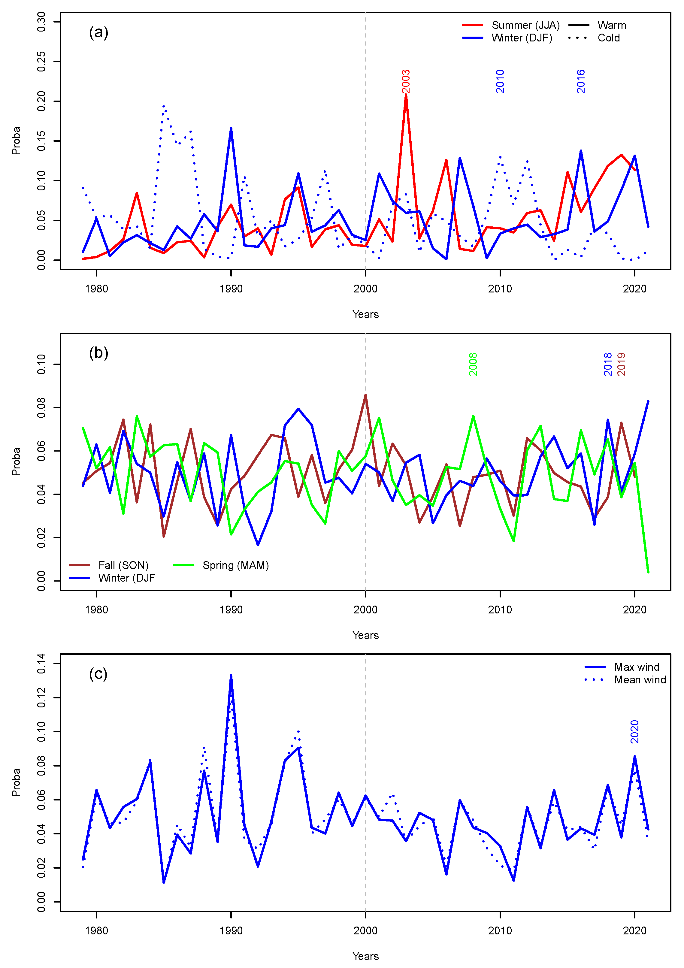
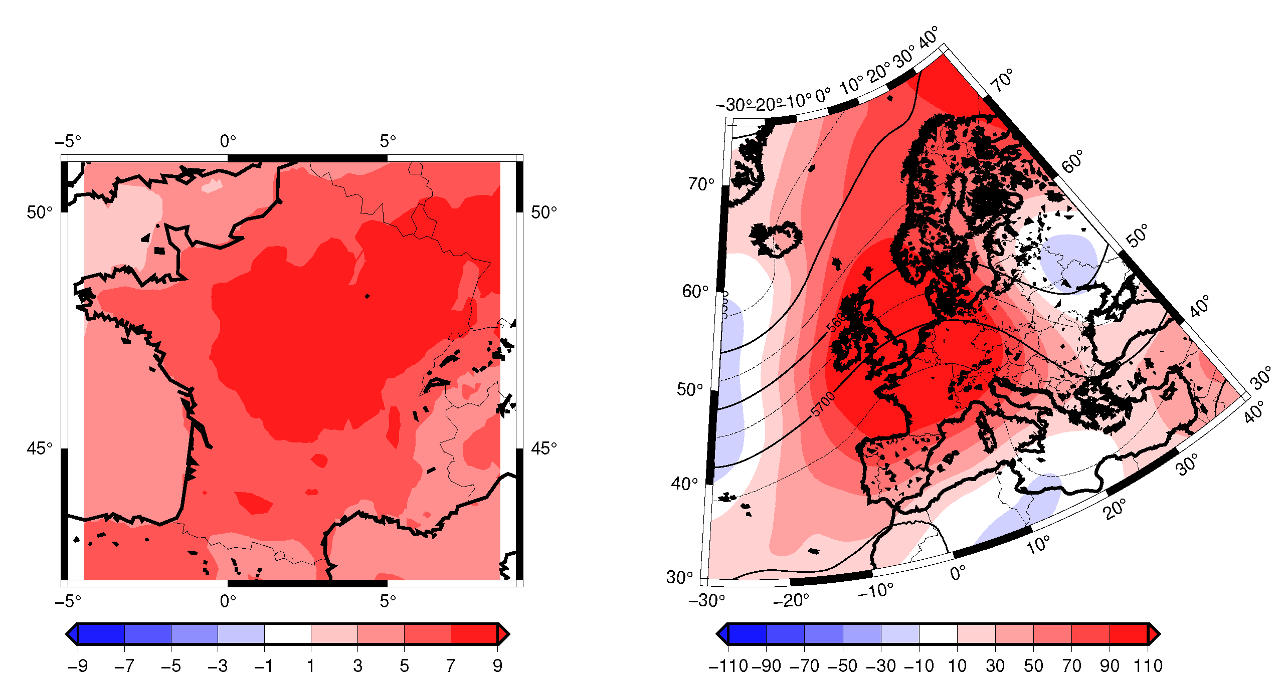
3.1. Summer Heatwaves
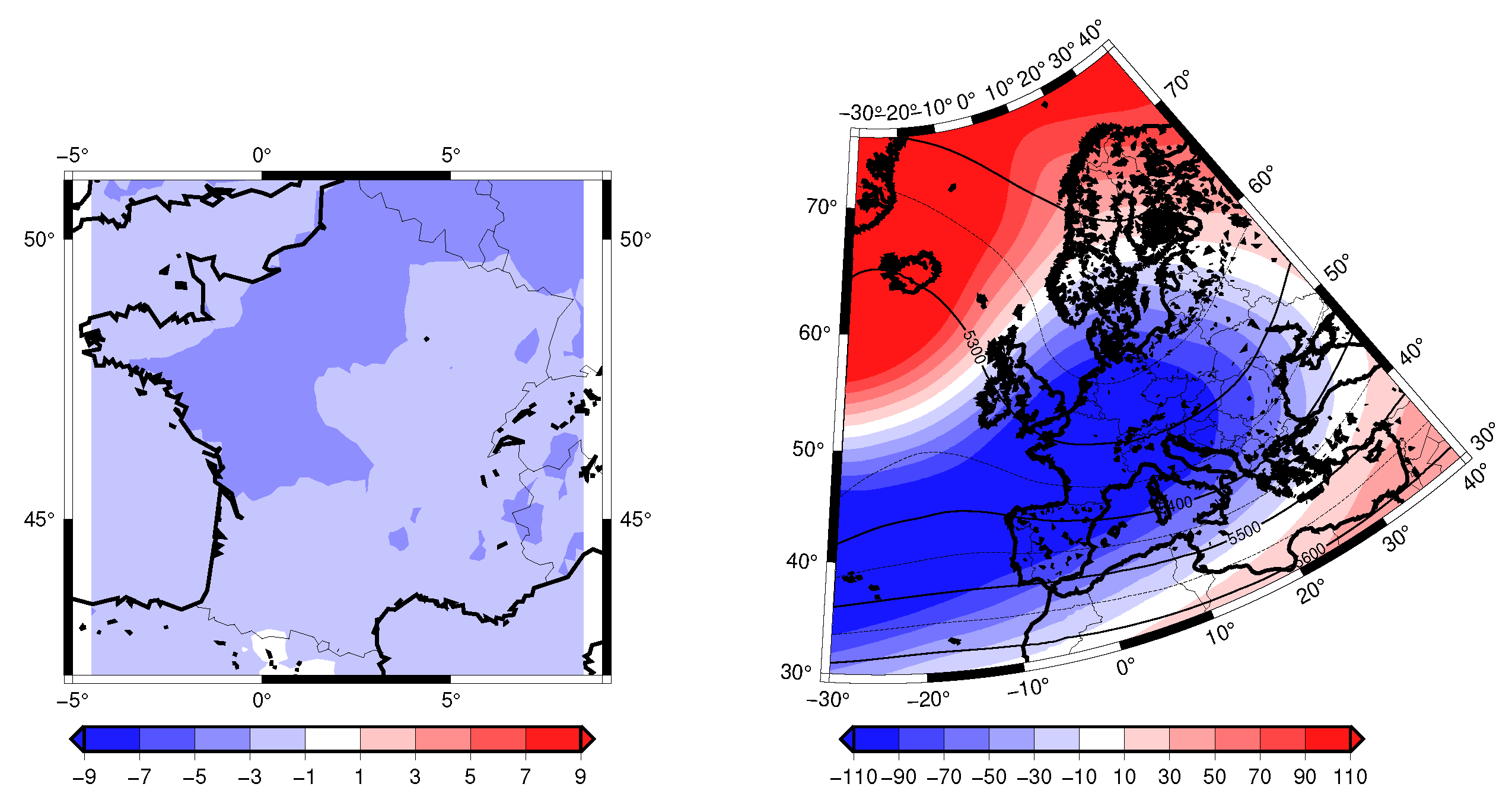
3.2. Winter Cold Spells
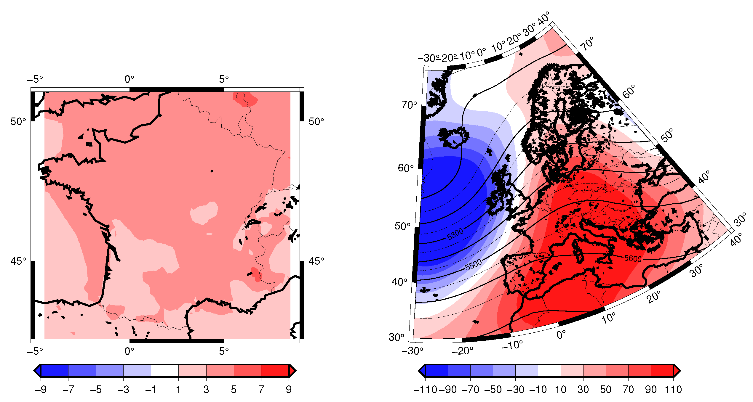
3.3. Winter Warm Spells
3.4. Wet Spring Events
3.5. Wet Winter Events
3.6. Autumn Mediterranean Events
3.7. Winter Storms
4. Methods
4.1. Bias Correction and Trend Removal
4.2. Variations of Dynamical Indicators due to Climate Change
4.2.1. Analogues Computation
4.2.2. Local Dimension
4.2.3. Local Persistence
4.2.4. Dynamical Indicators and Atmospheric Circulation
5. Results
5.1. Circulation for Temperature Extremes
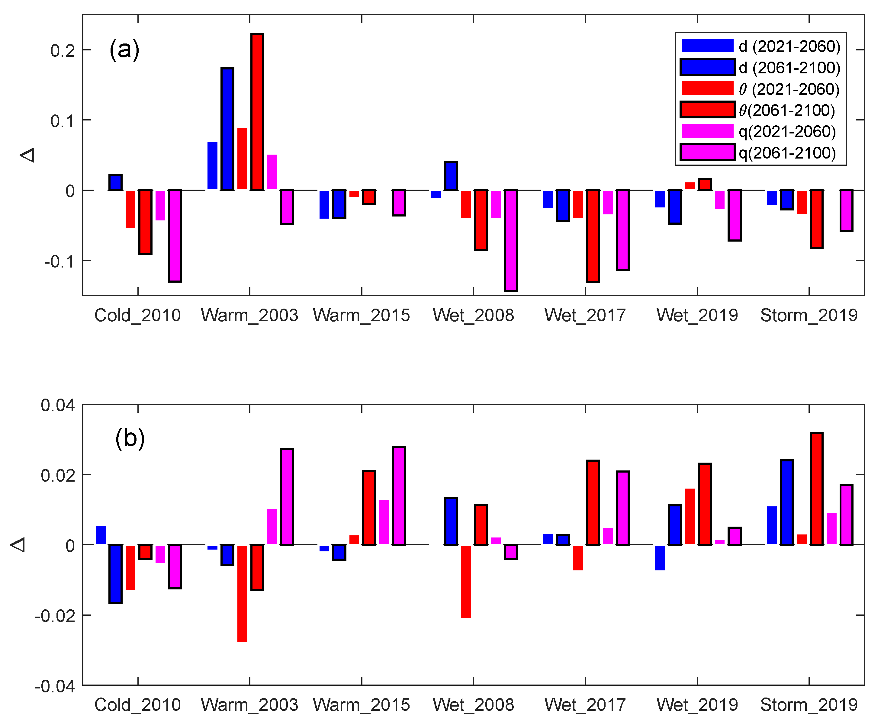
- Cold Spell 20210. From Figure 10, we see a modest change in the predictability, the persistence of this event increase in the future (negative variation of ). The analogue quality decreases, meaning that the event is less probable in future climate scenarios, in terms of atmospheric circulation (not just temperature).
- Heatwave 2003. With the trend (Figure 10a) we have an increase of dimension (decrease of predictability) and decrease of persistence and small relative trends for the analogues quality. When removing the Z500 trend (Figure 10b), the dimension does not change, while the persistence increases and the event becomes more probable
5.2. Circulation for Precipitation Extremes
- Wet spring 2008 and wet winter 2017. We see no trend in the dimension d. The persistence increases, and the quality of analogues decreases (Figure 10a). When removing the Z500 trend, we get contrasting signal in the metrics, in particular with better analogues and thus a higher probability of occurrence of the spatial patterns.
5.3. Circulation for a Wind Extreme
6. Discussion and Conclusions
Author Contributions
Funding
Data Availability Statement
Acknowledgments
Conflicts of Interest
Abbreviations
| CMIP6 | Coupled Model Intercomparison Project phase 6 |
| SSP585 | Socio-economic Pathway No. 5 with 8.5 W·m forcing |
| Z500 | Geopotential height at 500 hPa |
| SLP | Sea-level pressure |
| d | Local dimension |
| Persistence |
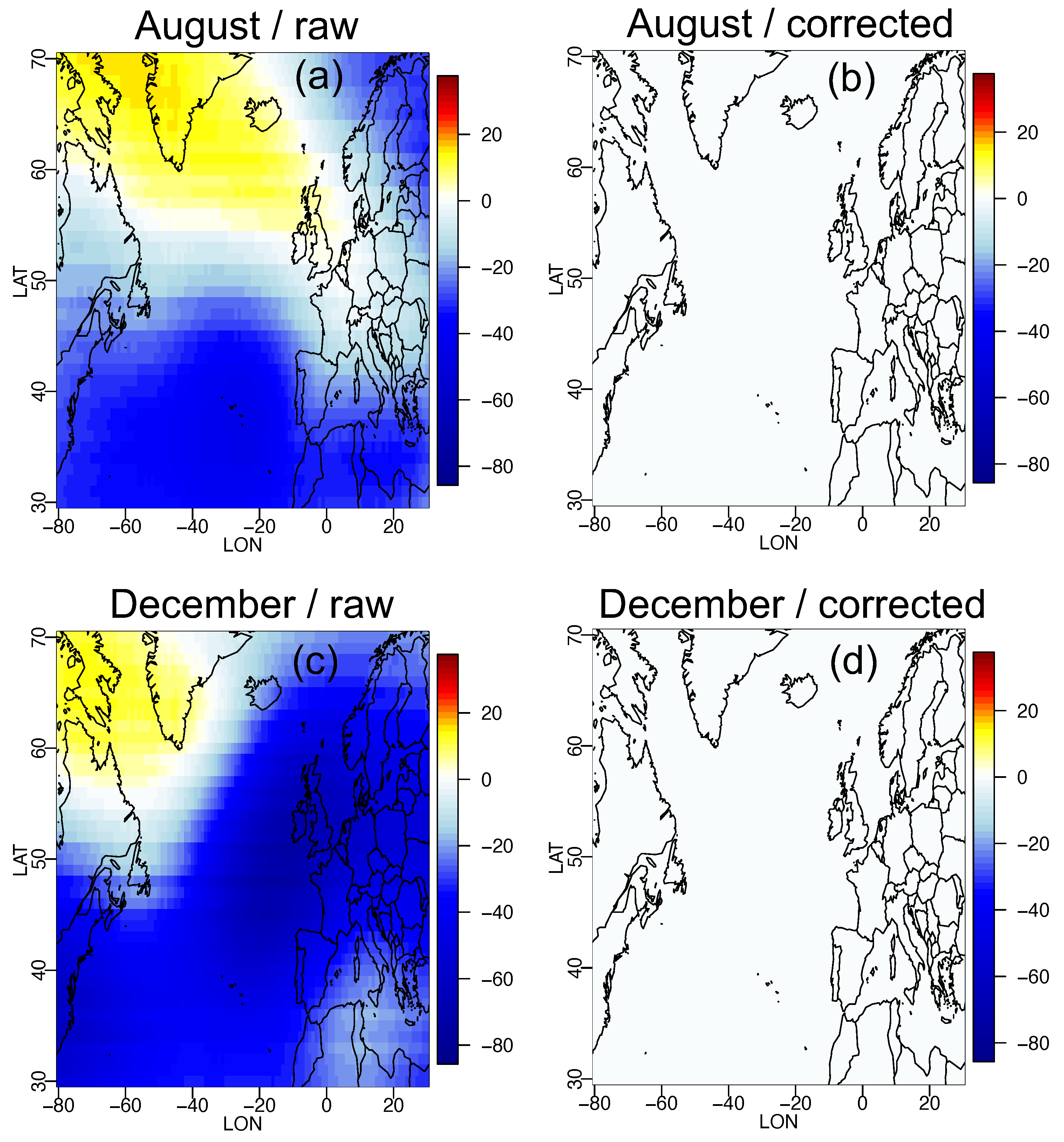
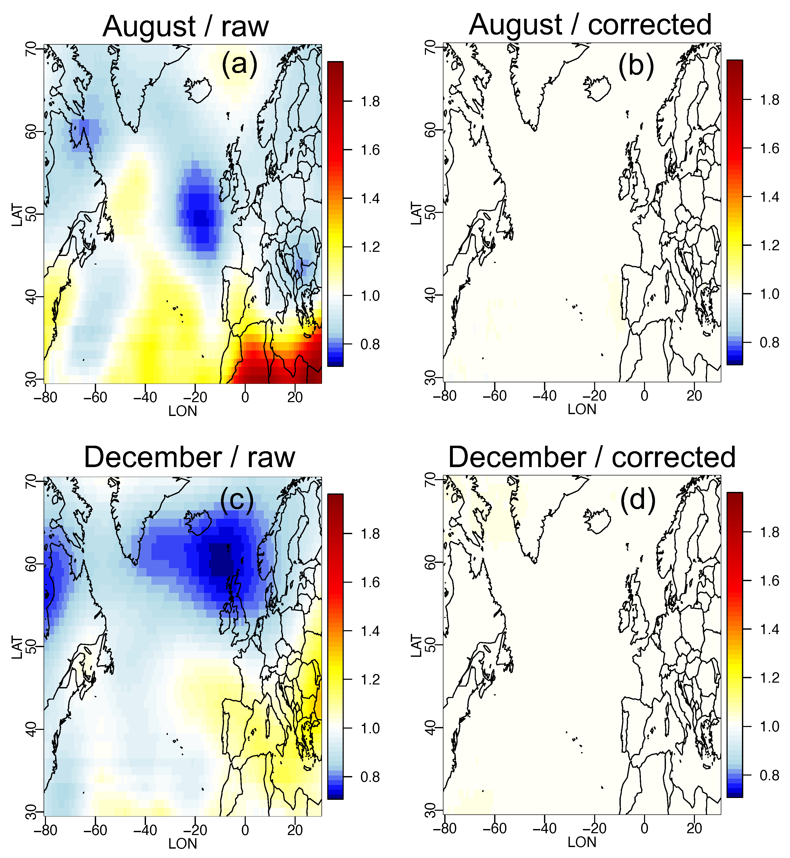
Appendix A. Quantification of Z500 Bias Correction


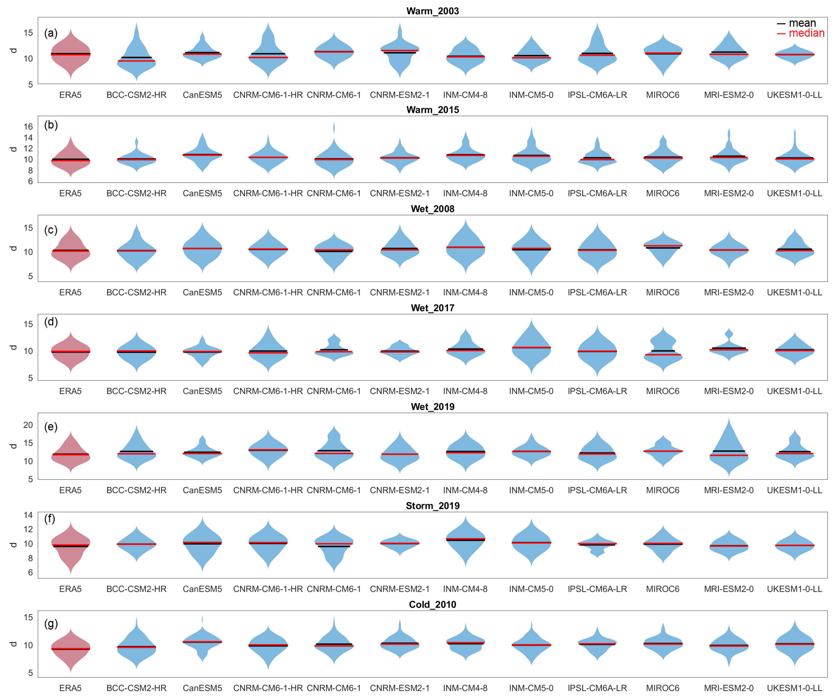
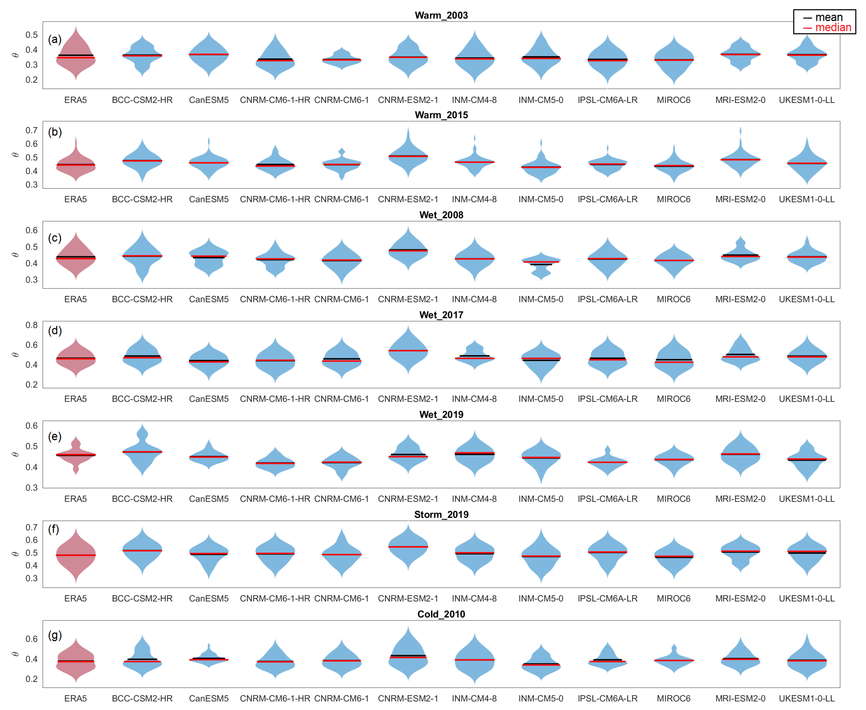
Appendix B. Distribution of d and θ for CMIP6


References
- Seneviratne, S.; Nicholls, N.; Easterling, D.; Goodess, C.; Kanae, S.; Kossin, J.; Luo, Y.; Marengo, J.; McInnes, K.; Rahimi, M.; et al. Changes in climate extremes and their impacts on the natural physical environment. In A Special Report of Working Groups I and II of the Intergovernmental Panel on Climate Change (IPCC SREX Report); Field, C., Barros, V., Stocker, T., Qin, D., Dokken, D., Ebi, K., Mastrandrea, M., Mach, K., Plattner, G.K., Allen, S., et al., Eds.; Cambridge University Press: Cambridge, UK, 2012. [Google Scholar]
- Jézéquel, A.; Dépoues, V.; Guillemot, H.; Trolliet, M.; Vanderlinden, J.P.; Yiou, P. Behind the veil of extreme event attribution. Clim. Chang. 2018, 149, 367–383. [Google Scholar] [CrossRef]
- Stott, P.A.; Christidis, N.; Otto, F.E.L.; Sun, Y.; Vanderlinden, J.P.; van Oldenborgh, G.J.; Vautard, R.; von Storch, H.; Walton, P.; Yiou, P.; et al. Attribution of extreme weather and climate-related events. Wiley Interdiscip. Rev. Clim. Chang. 2016, 7, 23–41. [Google Scholar] [CrossRef] [PubMed]
- National Academies of Sciences Engineering and Medicine (Ed.) Attribution of Extreme Weather Events in the Context of Climate Change; The National Academies Press: Washington, DC, USA, 2016. [Google Scholar] [CrossRef]
- Coles, S. An Introduction to Statistical Modeling of Extreme Values; Springer Series in Statistics; Springer: London, UK; New York, NY, USA, 2001. [Google Scholar]
- Shepherd, T.G. A Common Framework for Approaches to Extreme Event Attribution. Curr. Clim. Chang. Rep. 2016, 2, 28–38. [Google Scholar] [CrossRef]
- Yiou, P.; Jézéquel, A.; Naveau, P.; Otto, F.E.L.; Vautard, R.; Vrac, M. A statistical framework for conditional extreme event attribution. Adv. Stat. Climatol. Meteorol. Oceanogr. 2017, 3, 17–31. [Google Scholar] [CrossRef]
- Shepherd, T.G. Atmospheric circulation as a source of uncertainty in climate change projections. Nat. Geosci. 2014, 7, 703. [Google Scholar] [CrossRef]
- Faranda, D.; Vrac, M.; Yiou, P.; Jézéquel, A.; Thao, S. Changes in future synoptic circulation patterns: Consequences for extreme event attribution. Geophys. Res. Lett. 2020, 47, e2020GL088002. [Google Scholar] [CrossRef]
- Faranda, D.; Messori, G.; Yiou, P. Dynamical proxies of North Atlantic predictability and extremes. Sci. Rep. 2017, 7, 41278. [Google Scholar] [CrossRef]
- Lucarini, V.; Faranda, D.; Freitas, A.C.M.; Freitas, J.M.; Holland, M.; Kuna, T.; Nicol, M.; Todd, M.; Vaienti, S. Extremes and Recurrence in Dynamical Systems; John Wiley & Sons: Hoboken, NJ, USA, 2016. [Google Scholar]
- Caby, T.; Faranda, D.; Mantica, G.; Vaienti, S.; Yiou, P. Generalized dimensions, large deviations and the distribution of rare events. Phys. D-Nonlinear Phenom. 2019, 400, 132143. [Google Scholar] [CrossRef]
- Hurrell, J.; Kushnir, Y.; Ottersen, G.; Visbeck, M. (Eds.) Geophysical monograph. In The North Atlantic Oscillation: Climatic Significance and Environmental Impact; American Geophysical Union: Washington, DC, USA, 2003; Volume 134. [Google Scholar]
- Eyring, V.; Bony, S.; Meehl, G.A.; Senior, C.A.; Stevens, B.; Stouffer, R.J.; Taylor, K.E. Overview of the Coupled Model Intercomparison Project Phase 6 (CMIP6) experimental design and organization. Geosci. Model Dev. 2016, 9, 1937–1958. [Google Scholar] [CrossRef]
- Hersbach, H.; Bell, B.; Berrisford, P.; Hirahara, S.; Horányi, A.; Muñoz-Sabater, J.; Nicolas, J.; Peubey, C.; Radu, R.; Schepers, D. The ERA5 global reanalysis. Quat. J. Roy. Met. Soc. 2020, 146, 1999–2049. [Google Scholar] [CrossRef]
- Riahi, K.; Van Vuuren, D.P.; Kriegler, E.; Edmonds, J.; O’neill, B.C.; Fujimori, S.; Bauer, N.; Calvin, K.; Dellink, R.; Fricko, O. The Shared Socioeconomic Pathways and their energy, land use, and greenhouse gas emissions implications: An overview. Glob. Environ. Chang. 2017, 42, 153–168. [Google Scholar] [CrossRef]
- Wu, T.; Chu, M.; Dong, M.; Fang, Y.; Jie, W.; Li, J.; Li, W.; Liu, Q.; Shi, X.; Xin, X.; et al. BCC BCC-CSM2MR Model Output Prepared for CMIP6 CMIP piControl. Earth System Grid Federation. 2018. Available online: https://cera-www.dkrz.de/WDCC/ui/cerasearch/cmip6?input=CMIP6.CMIP.BCC.BCC-CSM2-MR.piControl (accessed on 27 September 2021). [CrossRef]
- Swart, N.C.; Cole, J.N.; Kharin, V.V.; Lazare, M.; Scinocca, J.F.; Gillett, N.P.; Anstey, J.; Arora, V.; Christian, J.R.; Jiao, Y.; et al. CCCma CanESM5 Model Output Prepared for CMIP6 ScenarioMIP. Earth System Grid Federation. 2019. Available online: https://cera-www.dkrz.de/WDCC/ui/cerasearch/cmip6?input=CMIP6.ScenarioMIP.CCCma.CanESM5 (accessed on 27 September 2021). [CrossRef]
- Voldoire, A. CNRM-CERFACS CNRM-CM6-1-HR Model Output Prepared for CMIP6 HighResMIP. Earth System Grid Federation. 2019. Available online: https://cera-www.dkrz.de/WDCC/ui/cerasearch/cmip6?input=CMIP6.HighResMIP.CNRM-CERFACS.CNRM-CM6-1-HR (accessed on 27 September 2021). [CrossRef]
- Voldoire, A. CNRM-CERFACS CNRM-CM6-1 Model Output Prepared for CMIP6 CMIP. Earth System Grid Federation. 2018. Available online: https://cera-www.dkrz.de/WDCC/ui/cerasearch/cmip6?input=CMIP6.CMIP.CNRM-CERFACS.CNRM-CM6-1 (accessed on 27 September 2021). [CrossRef]
- Seferian, R. CNRM-CERFACS CNRM-ESM2-1 Model Output Prepared for CMIP6 CMIP. Earth System Grid Federation. 2018. Available online: https://cera-www.dkrz.de/WDCC/ui/cerasearch/cmip6?input=CMIP6.CMIP.CNRM-CERFACS.CNRM-ESM2-1 (accessed on 27 September 2021). [CrossRef]
- Volodin, E.; Mortikov, E.; Gritsun, A.; Lykossov, V.; Galin, V.; Diansky, N.; Gusev, A.; Kostrykin, S.; Iakovlev, N.; Shestakova, A.; et al. INM INM-CM5-0 Model Output Prepared for CMIP6 CMIP abrupt-4xCO2. Earth System Grid Federation. 2019. Available online: https://cera-www.dkrz.de/WDCC/ui/cerasearch/cmip6?input=CMIP6.CMIP.INM.INM-CM5-0.abrupt-4xCO2 (accessed on 27 September 2021). [CrossRef]
- Boucher, O.; Denvil, S.; Levavasseur, G.; Cozic, A.; Caubel, A.; Foujols, M.A.; Meurdesoif, Y.; Cadule, P.; Devilliers, M.; Ghattas, J.; et al. IPSL IPSL-CM6A-LR Model Output Prepared for CMIP6 CMIP. Earth System Grid Federation. 2018. Available online: https://cera-www.dkrz.de/WDCC/ui/cerasearch/cmip6?input=CMIP6.CMIP.IPSL.IPSL-CM6A-LR (accessed on 27 September 2021). [CrossRef]
- Shiogama, H.; Abe, M.; Tatebe, H. MIROC MIROC6 Model Output Prepared for CMIP6 ScenarioMIP. Earth System Grid Federation. 2019. Available online: https://cera-www.dkrz.de/WDCC/ui/cerasearch/cmip6?input=CMIP6.ScenarioMIP.MIROC.MIROC6 (accessed on 27 September 2021). [CrossRef]
- Yukimoto, S.; Koshiro, T.; Kawai, H.; Oshima, N.; Yoshida, K.; Urakawa, S.; Tsujino, H.; Deushi, M.; Tanaka, T.; Hosaka, M.; et al. MRI MRI-ESM2.0 Model Output Prepared for CMIP6 CMIP. Earth System Grid Federation. 2019. Available online: https://cera-www.dkrz.de/WDCC/ui/cerasearch/cmip6?input=CMIP6.CMIP.MRI.MRI-ESM2-0 (accessed on 27 September 2021). [CrossRef]
- Tang, Y.; Rumbold, S.; Ellis, R.; Kelley, D.; Mulcahy, J.; Sellar, A.; Walton, J.; Jones, C. MOHC UKESM1.0-LL Model Output Prepared for CMIP6 CMIP Historical. Earth System Grid Federation. 2019. Available online: https://cera-www.dkrz.de/WDCC/ui/cerasearch/cmip6?input=CMIP6.CMIP.MOHC.UKESM1-0-LL.historical (accessed on 27 September 2021). [CrossRef]
- Cattiaux, J.; Ribes, A. Defining single extreme weather events in a climate perspective. Bull. Am. Meteorol. Soc. 2018, 99, 1557–1568. [Google Scholar] [CrossRef]
- Schaer, C.; Jendritzky, G. Climate change: Hot news from summer 2003. Nature 2004, 432, 559–560. [Google Scholar] [CrossRef] [PubMed]
- Schaer, C.; Vidale, P.; Luthi, D.; Frei, C.; Haberli, C.; Liniger, M.; Appenzeller, C. The role of increasing temperature variability in European summer heatwaves. Nature 2004, 427, 332–336. [Google Scholar] [CrossRef]
- Ciais, P.; Reichstein, M.; Viovy, N.; Granier, A.; Ogee, J.; Allard, V.; Aubinet, M.; Buchmann, N.; Bernhofer, C.; Carrara, A.; et al. Europe-wide reduction in primary productivity caused by the heat and drought in 2003. Nature 2005, 437, 529–533. [Google Scholar] [CrossRef]
- Vandentorren, S.; Suzan, F.; Medina, S.; Pascal, M.; Maulpoix, A.; Cohen, J.; Ledrans, M. Mortality in 13 French cities during the August 2003 heat wave. Amer. J. Public Health 2004, 94, 1518–1520. [Google Scholar] [CrossRef] [PubMed]
- García-León, D.; Casanueva, A.; Standardi, G.; Burgstall, A.; Flouris, A.D.; Nybo, L. Current and projected regional economic impacts of heatwaves in Europe. Nat. Commun. 2021, 12, 1–10. [Google Scholar]
- Poumadere, M.; Mays, C.; Le Mer, S.; Blong, R. The 2003 heat wave in France: Dangerous climate change here and now. Risk Anal. 2005, 25, 1483–1494. [Google Scholar] [CrossRef] [PubMed]
- Cattiaux, J.; Vautard, R.; Cassou, C.; Yiou, P.; Masson-Delmotte, V.; Codron, F. Winter 2010 in Europe: A cold extreme in a warming climate. Geophys. Res. Lett. 2010, 37. [Google Scholar] [CrossRef]
- Sillmann, J.; Croci-Maspoli, M.; Kallache, M.; Katz, R.W. Extreme cold winter temperatures in Europe under the influence of North Atlantic atmospheric blocking. J. Clim. 2011, 24, 5899–5913. [Google Scholar] [CrossRef]
- Hu, S.; Fedorov, A.V. The extreme El Niño of 2015–2016 and the end of global warming hiatus. Geophys. Res. Lett. 2017, 44, 3816–3824. [Google Scholar] [CrossRef]
- Yiou, P.; Vautard, R.; Naveau, P.; Cassou, C. Inconsistency between atmospheric dynamics and temperatures during the exceptional 2006/2007 fall/winter and recent warming in Europe. Geophys. Res. Lett. 2007, 34. [Google Scholar] [CrossRef]
- Cheung, H.H.; Zhou, W.; Leung, M.Y.; Shun, C.M.; Lee, S.M.; Tong, H.W. A strong phase reversal of the Arctic Oscillation in midwinter 2015/2016: Role of the stratospheric polar vortex and tropospheric blocking. J. Geophys. Res. Atmos. 2016, 121, 13443–13457. [Google Scholar] [CrossRef]
- Sousa, P.M.; Trigo, R.M.; Barriopedro, D.; Soares, P.M.; Santos, J.A. European temperature responses to blocking and ridge regional patterns. Clim. Dyn. 2018, 50, 457–477. [Google Scholar] [CrossRef]
- Ben-Ari, T.; Boé, J.; Ciais, P.; Lecerf, R.; Van der Velde, M.; Makowski, D. Causes and implications of the unforeseen 2016 extreme yield loss in the breadbasket of France. Nat. Commun. 2018, 9, 1627. [Google Scholar] [CrossRef]
- Vautard, R.; Colette, A.; Van Meijgaard, E.; Meleux, F.; Jan van Oldenborgh, G.; Otto, F.; Tobin, I.; Yiou, P. Attribution of Wintertime Anticyclonic Stagnation Contributing to Air Pollution in Western Europe. Bull. Am. Meteorol. Soc. 2018, 99, S70–S75. [Google Scholar] [CrossRef]
- Vautard, R.; Van Oldenborgh, G.J.; Otto, F.; Yiou, P.; De Vries, H.; Van Mijgaard, E.; Stepek, A.; Soubeyroux, J.M.; Philip, S.; Kew, S. Human influence on European winter wind storms such as those of January 2018. Earth Syst. Dyn. 2019, 10. [Google Scholar] [CrossRef]
- Ulbrich, U.; Leckebusch, G.C.; Pinto, J.G. Extra-tropical cyclones in the present and future climate: A review. Theor. Appl. Climatol. 2009, 96, 117–131. [Google Scholar] [CrossRef]
- Hoskins, B.J.; James, I.N. Fluid Dynamics of the Mid-Latitude Atmosphere; J. Wiley & Sons: Hoboken, NJ, USA, 2014. [Google Scholar]
- Michelangeli, P.A.; Vrac, M.; Loukos, H. Probabilistic downscaling approaches: Application to wind cumulative distribution functions. Geophys. Res. Lett. 2009, 36. [Google Scholar] [CrossRef]
- Vrac, M.; Drobinski, P.; Merlo, A.; Herrmann, M.; Lavaysse, C.; Li, L.; Somot, S. Dynamical and statistical downscaling of the French Mediterranean climate: Uncertainty assessment. Nat. Hazards Earth Syst. Sci. 2012, 12, 2769–2784. [Google Scholar] [CrossRef]
- Vigaud, N.; Vrac, M.; Caballero, Y. Probabilistic downscaling of GCM scenarios over southern India. Int. J. Climatol. 2013, 33, 1248–1263. [Google Scholar] [CrossRef]
- Ayar, P.V.; Vrac, M.; Bastin, S.; Carreau, J.; Déqué, M.; Gallardo, C. Intercomparison of statistical and dynamical downscaling models under the EURO-and MED-CORDEX initiative framework: Present climate evaluations. Clim. Dyn. 2016, 46, 1301–1329. [Google Scholar] [CrossRef]
- Vrac, M.; Noël, T.; Vautard, R. Bias correction of precipitation through Singularity Stochastic Removal: Because occurrences matter. J. Geophys. Res. Atmos. 2016, 121, 5237–5258. [Google Scholar] [CrossRef]
- Volosciuk, C.; Maraun, D.; Vrac, M.; Widmann, M. A combined statistical bias correction and stochastic downscaling method for precipitation. Hydrol. Earth Syst. Sci. 2017, 21, 1693–1719. [Google Scholar] [CrossRef]
- Van Oldenborgh, G.J.; Van Urk, A.; Allen, M. The absence of a role of climate change in the 2011 Thailand floods. Bull. Am. Meteor. Soc. 2012, 93, 1047–1049. [Google Scholar]
- Sweet, W.; Zervas, C.; Gill, S.; Park, J. Hurricane Sandy inundation probabilities today and tomorrow. Bull. Am. Meteorol. Soc. 2013, 94, S17–S20. [Google Scholar]
- Sweet, W.V.; Menendez, M.; Genz, A.; Obeysekera, J.; Park, J.; Marra, J.J. In tide’s way: Southeast Florida’s September 2015 sunny-day flood. Bull. Am. Meteorol. Soc. 2016, 97, S25–S30. [Google Scholar] [CrossRef]
- Kay, J.E.; Deser, C.; Phillips, A.; Mai, A.; Hannay, C.; Strand, G.; Arblaster, J.M.; Bates, S.C.; Danabasoglu, G.; Edwards, J. The Community Earth System Model (CESM) large ensemble project: A community resource for studying climate change in the presence of internal climate variability. Bull. Am. Meteorol. Soc. 2015, 96, 1333–1349. [Google Scholar] [CrossRef]
- Yoon, J.H.; Kravitz, B.; Rasch, P.J.; Simon Wang, S.Y.; Gillies, R.R.; Hipps, L. Extreme fire season in California: A glimpse into the future. Bull. Am. Meteorol. Soc. 2015, 96, S5–S9. [Google Scholar] [CrossRef]
- Jézéquel, A.; Bevacqua, E.; d’Andrea, F.; Thao, S.; Vautard, R.; Vrac, M.; Yiou, P. Conditional and residual trends of singular hot days in Europe. Environ. Res. Lett. 2020, 15, 064018. [Google Scholar] [CrossRef]
- Freitas, A.C.M.; Freitas, J.M.; Todd, M. Hitting time statistics and extreme value theory. Probab. Theory Relat. Fields 2010, 147, 675–710. [Google Scholar] [CrossRef]
- Lucarini, V.; Kuna, T.; Wouters, J.; Faranda, D. Relevance of sampling schemes in light of Ruelle’s linear response theory. Nonlinearity 2012, 25, 1311. [Google Scholar] [CrossRef][Green Version]
- Liebovitch, L.S.; Toth, T. A fast algorithm to determine fractal dimensions by box counting. Phys. Lett. A 1989, 141, 386–390. [Google Scholar] [CrossRef]
- Sarkar, N.; Chaudhuri, B.B. An efficient differential box-counting approach to compute fractal dimension of image. IEEE Trans. Syst. Man Cybern. 1994, 24, 115–120. [Google Scholar] [CrossRef]
- Süveges, M. Likelihood estimation of the extremal index. Extremes 2007, 10, 41–55. [Google Scholar] [CrossRef]
- Yiou, P.; Cattiaux, J.; Faranda, D.; Kadygrov, N.; Jézéquel, A.; Naveau, P.; Ribes, A.; Robin, Y.; Thao, S.; van Oldenborgh, G.J. Analyses of the Northern European summer heatwave of 2018. Bull. Am. Meteorol. Soc. 2020, 101, S35–S40. [Google Scholar] [CrossRef]
- Taylor, K.E.; Stouffer, R.J.; Meehl, G.A. An Overview of CMIP5 and the Experiment Design. Bull. Amer. Met. Soc. 2012, 93, 485–498. [Google Scholar] [CrossRef]
- Kistler, R.; Kalnay, E.; Collins, W.; Saha, S.; White, G.; Woollen, J.; Chelliah, M.; Ebisuzaki, W.; Kanamitsu, M.; Kousky, V.; et al. The NCEP-NCAR 50-year reanalysis: Monthly means CD-ROM and documentation. Bull. Am. Meteorol. Soc. 2001, 82, 247–267. [Google Scholar] [CrossRef]
- Yiou, P.; Nogaj, M. Extreme climatic events and weather regimes over the North Atlantic: When and where? Geophys. Res. Lett. 2004, 31, L07202. [Google Scholar] [CrossRef]
- Cassou, C.; Terray, L.; Phillips, A.S. Tropical Atlantic influence on European heat waves. J. Clim. 2005, 18, 2805–2811. [Google Scholar] [CrossRef]
- Robin, Y.; Yiou, P.; Naveau, P. Detecting changes in forced climate attractors with Wasserstein distance. Nonlinear Process. Geophys. 2017, 24, 393–405. [Google Scholar] [CrossRef]
- Vrac, M.; Ayar, P.V.; Yiou, P. Trends and variability of seasonal weather regimes. Int. J. Climatol. 2013. [Google Scholar] [CrossRef]
- Faranda, D.; Alvarez-Castro, M.C.; Messori, G.; Rodrigues, D.; Yiou, P. The hammam effect or how a warm ocean enhances large scale atmospheric predictability. Nat. Commun. 2019, 10, 1316. [Google Scholar] [CrossRef]
- Yiou, P.; Servonnat, J.; Yoshimori, M.; Swingedouw, D.; Khodri, M.; Abe-Ouchi, A. Stability of weather regimes during the last millennium from climate simulations. Geophys. Res. Lett. 2012, 39. [Google Scholar] [CrossRef]
- Vautard, R.; Yiou, P.; Otto, F.; Stott, P.; Christidis, N.; Oldenborgh, G.J.V.; Schaller, N. Attribution of human-induced dynamical and thermodynamical contributions in extreme weather events. Environ. Res. Lett. 2016, 11, 114009. [Google Scholar] [CrossRef]
- Schaller, N.; Kay, A.L.; Lamb, R.; Massey, N.R.; van Oldenborgh, G.J.; Otto, F.E.L.; Sparrow, S.N.; Vautard, R.; Yiou, P.; Ashpole, I.; et al. Human influence on climate in the 2014 southern England winter floods and their impacts. Nat. Clim. Chang. 2016, 6, 627–634. [Google Scholar] [CrossRef]


| Simulation Name | Atmospheric Resolution | Data Reference |
|---|---|---|
| BCC-CSM2-MR | 100 km | [17] |
| CanESM5 | 500 km | [18] |
| CNRM-CM6-1-HR | 100 km | [19] |
| CNRM-CM6-1 | 250 km | [20] |
| CNRM-ESM2-1 | 250 km | [21] |
| INM-CM4-8 | 100 km | [22] |
| INM-CM5-0 | 100 km | [22] |
| IPSL-CM6A-LR | 250 km | [23] |
| MIROC6 | 250 km | [24] |
| MRI-ESM2-0 | 100 km | [25] |
| UKESM1-0-LL | 250 km | [26] |
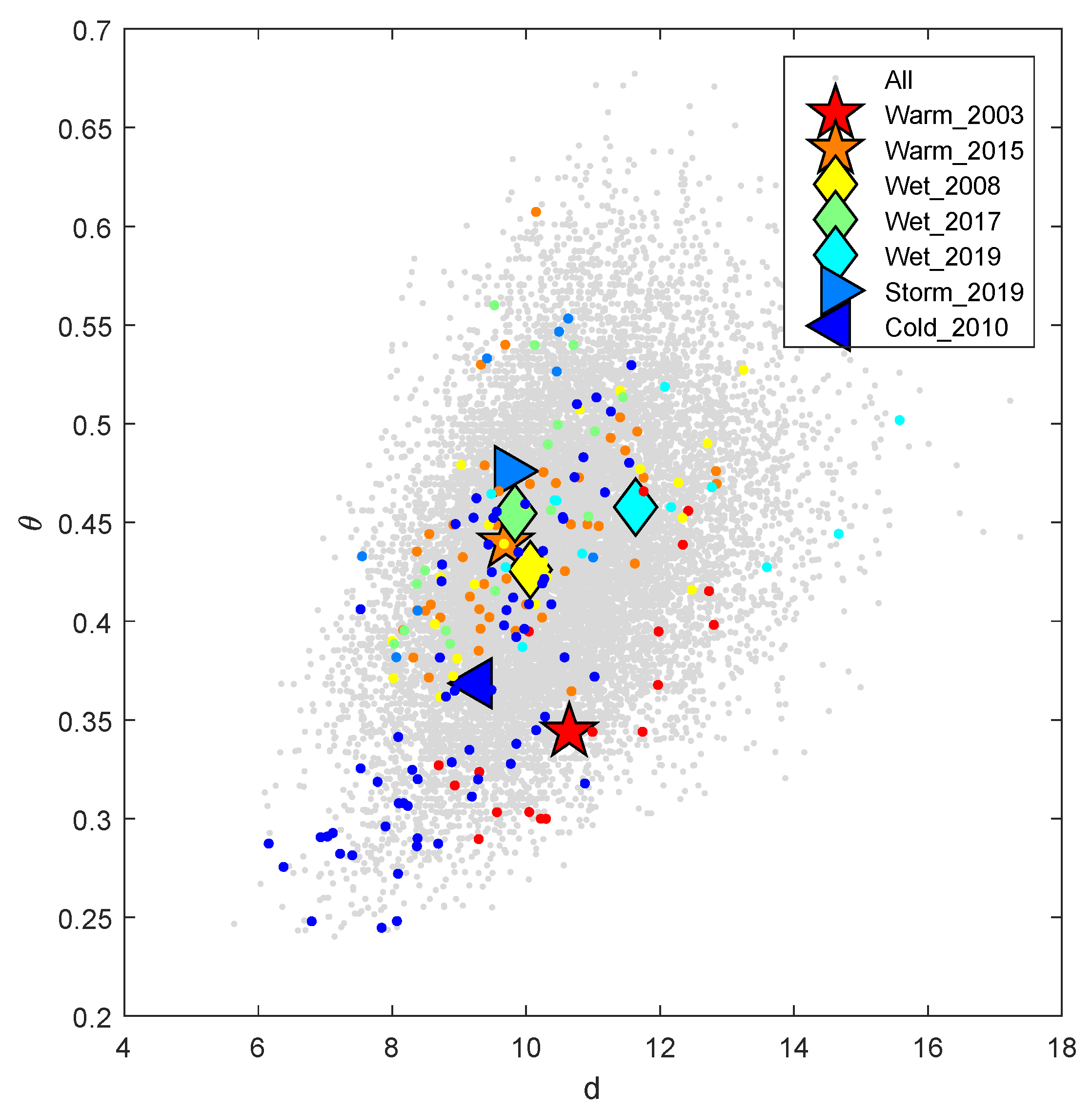
| Date of Event | Cold | Warm | Wet | Storm | d | |
|---|---|---|---|---|---|---|
| 31 July 2003–17 August 2003 | X | 10.64 | 0.34 | |||
| 09 March 2008–01 April 2008 | X | 10.06 | 0.43 | |||
| 11 December 2009–18 February 2010 | X | 9.27 | 0.37 | |||
| 01 December 2015–13 January 2016 | X | 9.70 | 0.44 | |||
| 25 December 2017–09 January 2018 | X | 9.83 | 0.45 | |||
| 13 October 2019–25 October 2019 | X | 11.63 | 0.46 | |||
| 06 December 2019–15 December 2019 | X | X | 9.75 | 0.48 |
Publisher’s Note: MDPI stays neutral with regard to jurisdictional claims in published maps and institutional affiliations. |
© 2021 by the authors. Licensee MDPI, Basel, Switzerland. This article is an open access article distributed under the terms and conditions of the Creative Commons Attribution (CC BY) license (https://creativecommons.org/licenses/by/4.0/).
Share and Cite
Yiou, P.; Faranda, D.; Thao, S.; Vrac, M. Projected Changes in the Atmospheric Dynamics of Climate Extremes in France. Atmosphere 2021, 12, 1440. https://doi.org/10.3390/atmos12111440
Yiou P, Faranda D, Thao S, Vrac M. Projected Changes in the Atmospheric Dynamics of Climate Extremes in France. Atmosphere. 2021; 12(11):1440. https://doi.org/10.3390/atmos12111440
Chicago/Turabian StyleYiou, Pascal, Davide Faranda, Soulivanh Thao, and Mathieu Vrac. 2021. "Projected Changes in the Atmospheric Dynamics of Climate Extremes in France" Atmosphere 12, no. 11: 1440. https://doi.org/10.3390/atmos12111440
APA StyleYiou, P., Faranda, D., Thao, S., & Vrac, M. (2021). Projected Changes in the Atmospheric Dynamics of Climate Extremes in France. Atmosphere, 12(11), 1440. https://doi.org/10.3390/atmos12111440