Article

Impacts of Vegetation and Topography on Land Surface Temperature Variability over the Semi-Arid Mountain Cities of Saudi Arabia

1
Department of Architecture and Planning, College of Engineering, King Khalid University, Abha 61411, Saudi Arabia
2
Department of Civil Engineering, College of Engineering, King Khalid University, Abha 61411, Saudi Arabia
3
Department of Energy and Environment, TERI School of Advanced Studies, New Delhi 110070, India
4
Urban Environmental & Remote Sensing, Natural Science, Jamia Millia Islamia, New Delhi 110025, India
*
Author to whom correspondence should be addressed.
Atmosphere 2020, 11(7), 762; https://doi.org/10.3390/atmos11070762
Submission received: 14 June 2020 / Revised: 14 July 2020 / Accepted: 16 July 2020 / Published: 18 July 2020
(This article belongs to the Special Issue Interaction between Urban Microclimates and the Buildings)

Abstract

:
Land surface temperature (LST) can fully reflect the water–heat exchange cycle of the earth surface that is important for the study of environmental change. There is little research on LST in the semi-arid region of Abha-Khamis-Mushyet, which has a complex topography. The study used LST data, retrieved from ASTER data in semi-arid mountain areas and discussed its relationship with land use/land cover (LULC), topography and the normalized difference vegetation index (NDVI). The results showed that the LST was significantly influenced by altitude and corresponding LULC type. In the study area, during the summer season, extreme high-temperature zones were observed, possibly due to dense concrete surfaces. LST among different types of land use differed significantly, being the highest in exposed rocky areas and built-up land, and the lowest in dense vegetation. NDVI and LST spatial distributions showed opposite trends. The LST–NDVI feature space showed a unique ABC obtuse-angled triangle shape and showed an overall negative linear correlation. In brief, the LST could be retrieved well by the emissivity derived NDVI TES method, which relied on upwelling, downwelling, and transmittance. In addition, the LST of the semi-arid mountain areas was influenced by elevation, slope zenith angle, aspect and LULC, among which vegetation and elevation played a key role in the overall LST. This research provides a roadmap for land-use planning and environmental conservation in mountainous urban areas.

1. Introduction

Mountains are well-known drivers of climate change and growth in global mass and energy balance. Extreme topographical variability introduced in mountain areas creates complex spatial–temporal patterns of meteorological and hydrological process, and ecological parameters with high gradients of attitude at short distances [1,2,3,4]. Mountain ecosystems are also very vulnerable to natural and anthropogenic changes, compared to lowland ecosystems. Mountain ecosystem restoration from disruptions is usually slow or failing. Analysis of atmospheric surface processes in mountain regions has become an integral aspect of mountain environment research, to quantitatively understand the role of mountain climate, its status and trends.
Satellite-borne thermal infrared remote (TIR) sensors receive electromagnetic radiation (EMR) that can be directly measured as Top of Atmosphere (TOA) radiance measurements. The TOA radiances are transformed to LST by correction for three major influences; angular effects [5], atmospheric absorption and scattering [6], and surface spectral emissivity values [7]. Such corrections are carried out using complex algorithms, alongside thorough validation and evaluation, resulting in a final product that a climate scientist might use [8].
Satellite-borne TIR data are connected directly to the LST through the radiative transfer equation. LST retrieval from TIR data received extensive interest, and its history dates from the 1970s [9]. In an attempt to comprehend the Earth system on a regional scale and to have the evapotranspiration with accuracy better than 10%, LST must be derived at an accuracy of 1 K or more [10]. Even so, it is difficult to make a direct LST estimation of the radiation emitted in the spectral region of the TIR with high accuracy, as radiation measured by radiometers onboard satellites depends not only on surface parameters (temperature and emissivity), but also on atmospheric conditions [11]. Thus, in addition to radiometric calibration and cloud cover analysis, the estimation of LSTs from space-based TIR observations requires both atmospheric correction and surface emissivity [12]. A number of studies were performed, and various techniques were suggested to retrieve LSTs from satellite TIR data, using a range of methods to mitigate emissivity and atmospheric impacts [7,10,13,14,15,16,17,18,19,20,21,22]. The retrieving LST and relationship with biophysical parameters were studied by Mallick [23], El-Nahry and Rashash [24], Ali and Mohammed [25]; Mujabar and Rao [26]; and Sheik Mujabar [27].
Land surface temperature (LST) is a crucial factor in the control of interface energy transfers during surface–atmosphere exchange [28,29]. Remote sensing is based on the temperature of the Earth’s surface shell called skin temperature, which is available for the entire earth surface [30]. Remote sensing related LST products have a surface skin kinetic temperature estimate [31]. Several researchers used remote sensing technology to estimate and understand LST [29,32]. Vlassova et al. [33] stated that LST is one of the main inputs of soil vegetation modelling in terrestrial ecosystems. LST relates to the heat transfer between the earth’s surface and the atmospheric boundary layer [34,35] and enables sensitive heat flux estimation [36] and evapotranspiration or latent heat flux [37]. Linh et al. [38] reported that monitoring of LST in densely populated areas is problematic, as the relatively high density and continuous operation of meteorological stations in these areas are not feasible. Spatio-temporal heterogeneity of surface energy fluxes suggests variations in LST at various spatial and temporal scales; commonly used in a broad wide range of studies of the environmental field, including surface energy budget analysis [39,40,41,42], vegetation monitoring [43], hydrological cycle [44,45,46], and urban thermal environmental studies [47,48].
LST information offers useful information on major water and heat-related land-surface processes in the mountain areas. The spatial–temporal variations of the LST in the mountainous area, however, are highly affected by meteorological impacts, topographical gradients, and altitude zoning. Among such results, topography exhibited significant effects as observed by the difference in surface illumination under various aspects and slopes. Consequently, the complex LST trend poses key constraints in the determination of surface energy exchanges in the mountains, and significantly restricts the application of land surface temperature. For example, in previous studies of evapotranspiration; mountain pixels with topography far away from average altitude were evaluated to avoid misdefined well-watered pixels [49,50]. Although surface energy and heat flux techniques are estimated well over the specific area, the omission of the relatively low or high elevation surface cannot satisfy the requirements under different topographical conditions.
Developing remote sensing techniques to incorporate LST knowledge and other ecological variables from different spatiotemporal scales provide a vital means of determining LST’s spatial–temporal pattern and evolving framework. Van De Kerchove et al. [1] performed a spatial–temporal variations assessment, based on data from the MODIS LST time-series in the Russian Altay Mountains. The correlation between the five physiographical variables (solar insolation, topographical integration, elevation, vegetation, and duration of snow cover) and important LST-derived Fourier components was studied, with specific effects on the day and night, as well as the diurnal variation. Stroppiana et al. [51] also analyzed the impact of elevation and land use/land cover on spatiotemporal LST changes from MODIS data, to better understand the nature of the LST relationship and its influencing forces.
Studies on the retrieval of LST were performed over the past few decades, using high and medium resolution satellites such as Landsat, ASTER, MODIS, and others [19,20,22,52]. Nonetheless, several studies noted that LST retrieval using medium- and low-resolution satellite data has many spectral and spatial limitations affecting its accuracy. In Saudi Arabia, the retrieval of LST and the relationship to biophysical parameters (i.e., NDVI) were also used [23,24,25,26,27]. This study aimed to analyze the algorithms used to extract LST from NASA’s Terra ASTER sensor, using the VNIR channels and TIR channels. While these algorithms currently exist, their use in LST retrieval is not a simple process. Due to the complexity of incorporating these algorithms into the currently available software, and the cost of procuring geographic information systems and image processing software, a lot of consumers are still unable to execute such algorithms. A ready-to-use LST retrieval method not only promotes the use of an efficient algorithm but also allows a user to use sensor data in a variety of many other areas.
A rise in vegetation areas is the critical alternative for local climate mitigation [53]. This is because the atmosphere is controlled mainly by shading [54], CO2 sequestration [55], and evapotranspiration [56]. Densely vegetated areas have a general declining trend in the LST (exhibited by the rise in NDVI), as it prevents incident solar radiation and increases the evaporative cooling effect of the vegetation, which reduces an increase in surface temperature [23,57,58,59]. The terrain impact evaluation on the LST indicates that the change in temperature pattern shows significant variations with respect to the main factors associated with elevation, vegetation cover, and solar radiation [57].
LST is an essential element that reflects changes in the environment, in the landscape, and the physical processes underlying the semi-arid urban mountain area. Thus, it is necessary to evaluate LST retrieval by using the proportion of vegetation cover in conjunction with normalized difference vegetation index (NDVI) and integrate it into the Temperature and Emissivity Separation (TES) algorithm, and the impact of LST and LULC, NDVI and topographical parameters in semi-arid mountainous areas should also be explored. To reveal land surface temperature characteristics in semi-arid mountainous regions, we have chosen a typical urban environment, i.e., Abha-Khamis-Mushayet Twin Cities, Asir Province, and Saudi Arabia, as a study area; and estimated the LST and NDVI from ASTER to assess the aforementioned problems. Meanwhile, the LULC was generated by the MLC classification technique. The objectives of this study were (1) analyze LST spatial distribution characteristics and accuracy in the study area using proportion of vegetation cover in conjunction with NDVI and integrate it into the TES algorithm and validate the accuracy level based on ground-measurement (in-situ); (2) investigate the relationship between LST and its impact factors in mountainous semi-arid urban areas, (3) evaluate the relationship between LST and LULC while considering the elevation; and (4) determine the relationship between NDVI and LST.

2. Study Area

The area selected for this research was the Abha-Khamis-Mushayet Twin Cities (Figure 1) in the South-Western province of Saudi Arabia. The urban high hills are a vital tourist area with the richest biodiversity of flora and fauna in the Asir region and KSA [60]. The study site had a total area of 1291 km2 (Figure 1) and a vegetation type dominated by J. procera trees, Acacia origena and A. gerrardii. Geographically, the Abha-Khamis-Mushayet twin cities extend between 18°9′33.126″ N and 18°30′56.566″ N latitudes and 42°23′52.477″ E to 42°51′42.832″ E longitude, and the elevation varied from 1564 m to 2736 m with a mean of 2102 m at the mean sea level. As per the Saudi Geological Society, the study area had hard silt, soft clay, and sedimentary soil. The study area had a heterogeneous landscape in terms of the terrain complexity. It was situated in an essential zone of Afromontane, where cold and semi-arid climates characterize the city’s environment [61]. The mean annual rainfall for the last 55 years (1965–2019) was 245 mm, among which most of the precipitation occurred during the months of February to June, while the mean minimum and maximum air temperature were 9.4 °C and 30.8 °C, respectively. The watershed is vulnerable to high-intensity rainfall, and several rural areas undergo flash flooding in or during the winter season [62].

3. Methodology

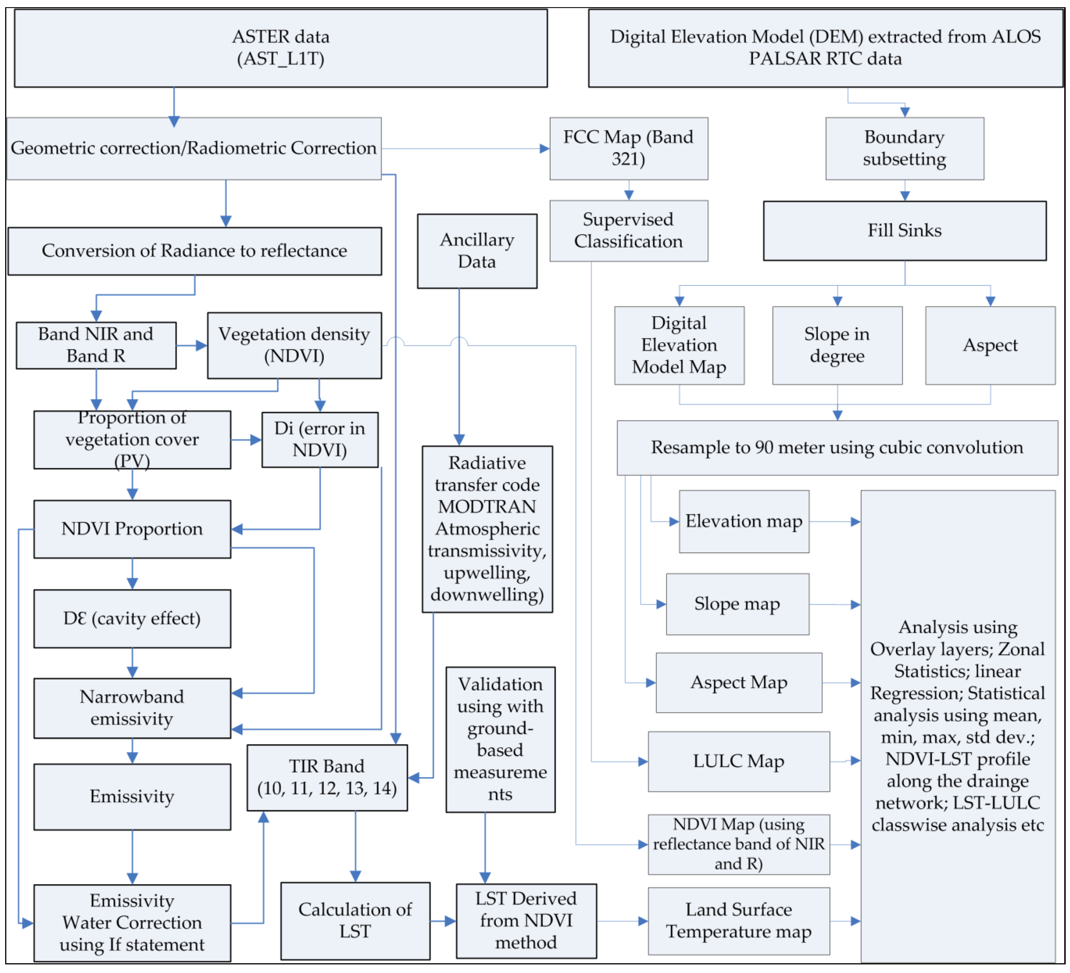
In this study, ASTER was used and radiometric calibration and geometric co-registration was carried out and used for the preparation of land use/land cover, vegetation density map (NDVI), and estimating the LST. Topographic elevation map was developed for the study area using the Digital Elevation Model (DEM) obtained from ALOS PALSAR RTC data [63]. The raw DEM data was processed by filling the sinks to cover local depressions. Slope, aspect, and drainage network maps were derived directly from the elevation data (i.e., DEM). A field survey was conducted from 24–27 June 2019, comparing the estimated satellite surface temperature values with ground-based measurements (in-situ). The ArcGIS and image processing software, i.e., ArcGIS 10.3, ENVI 4.8, ERDAS imagine 9.2, FLAASH 4.8, and Microsoft Office 2010 software and statistics computation, SPSS 24 software were used to carry out this study. For field observations of surface temperature, infrared thermometer and Garmin-GPS were used. Figure 2 demonstrates the flow diagram for the adopted methodology.

3.1. ASTER Sensor

ASTER is a multi-spectral high-spatial-resolution image that was launched on NASA’s Terra spacecraft in 1999, which transmits data from a visible to the thermal infrared region, covering an area of 3600 km2 in 14 spectral bands. ASTER comprises three different spectral band categories; in the first category there are four bands with a spatial resolution of 15 m in the region of visible and near-infrared (VNIR); in the second category there are 6 bands with a spatial resolution of 30 m in the region of shortwave infrared (SWIR); and in the third category, there are five bands with a spatial resolution of 90 m in the region of thermal infrared (TIR) [64].

3.2. Radiometric Calibration

Radiometric calibration is crucial to the development of high-quality scientific data. The ability to detect and quantify changes in the Earth’s environment depends on the sensors, which can quantify the surface of the earth over time. A comprehensive description of scientific data from a global range of remote sensor data requires the identification of product artefacts and the study of earth process changes [65]. Determining the spectral emission of the sensor is the crucial step for the transfer of image data from the number of sensors to a standard radiometric scale. “The radiometric calibration of the ASTER sensors involve the rescaling of the raw digital numbers (Q) transmitted from the satellite to the calibrated digital numbers (Qcal), using the same radiometric scale for all scenes processed on the ground for a specific period”.
Digital number (DN) values conversion to radiance (at-sensor) using Equation (1) is expressed in Wm 2 sr 1 μ m 1 .
L λ = ( D N 1 ) * U C C
“where, UCC is unit conversion coefficients from the HDF file” (Source: ASTER User Handbook [42]).

3.3. Atmospheric Correction for the ASTER Channel

The electromagnetic energy that goes through the atmosphere attenuates the radiation before reaching the sensor. Therefore the elimination of the atmospheric influences is important. ASTER’s atmospheric thermal data correction uses a clear-sky approach that cannot be applied near the clouds. This is based on the equation of radiative transfer and uses the “MODerate resolution atmospheric TRANsmission (MODTRAN)”, Version 3.5 radiative transfer code. The system includes all the required standard atmospheric and geometric parameters, including temperature, channel reflection, water vapor, aerosol, CO2 mixing ratio (ppm), ozone, number of disort stream, radiance image scale factor, etc. This atmospheric module used an algorithm that was based on observations by Kaufman et al. [6], and the parameters were associated with each image’s geometry as input for atmospheric correction. For more information, please see Palluconi et al. [66].

3.4. Retrieval of Emissivity and LST

In terms of emissivity variation, natural surfaces at a pixel scale are not homogeneous. The surface emissivity value of Earth shows a strong seasonal presence and dependence on the landscape. “Emissivity depends in particular on the type of land cover, soil moisture, organic soil composition, vegetation density and structure i.e., broadband emissivity for densely vegetated areas, which are usually around 0.96–0.98, but for bare soils, it can be lower than 0.90 [67]” because of the variations in TES’s scaling of high-low MMD emissivity spectra. It is appropriate, irrespective of the TIR data, to use ASTER’s VNIR data to estimate vegetation proportion cover and surface emissivity. Various methods for determining emissivity from NDVI were formulated [58,68,69].
ASTER satellite data were used to derive the land surface emissivity (LSE) by taking the vegetation cover ratio per pixel in combination with NDVI. The “proportion of vegetation cover” was calculated as given in Equation (2) [70]:
P v = ( 1 i i g ) ( 1 i i g ) k ( 1 i i v )
“where, i g = NDVI value of pure soil; i v = NDVI value of pure vegetation pixel; i is the NDVI value of mixed pixels”.
k = ( ρ N I R v ρ R E D v ) ( ρ N I R g ρ R E D g )
“where ρ N I R v ρ R E D v are reflectance in the NIR (band5) and red (band4) for pure pixels of vegetation; ρ N I R g ρ R E D g are reflectance in the NIR (band5) and red (band4) for pure pixels of the soil, respectively”.
For this, the model had two phases—in the first phase, the pure pixel vegetation and the bare soil properties were derived from the NDVI, and in the second phase, the emissivity was determined by integrating the vegetation cover proportion per pixel with the NDVI and the emissivity value error estimate. The proportion of mixed pixel NDVI (consisting of mixed pixels of vegetation and bare soil) was calculated in Equation (4) below
N D V I = ( i v * P v ) + i g ( 1 P v ) + d i
“where, i v Pure pixel of vegetation NDVI; i g Pure pixel of soil NDVI; d i NDVI error”
The “emissivity and cavity effects” was estimated as mentioned below, using Equations (5) and (6)
ε ( 8 14 ) = ( ε v ε s i v i g ) * N D V I + ( ε s ( i v + d i ) ε v ( i g + d i ) ( i v i g ) ) + d ε
where Δ ε was calculated from Equation (6)
d ε = ( 1 ε s ) ε v F ( 1 P v ) + ( 1 P v ) ε s G + ( 1 ε v ) ε v F ´ P s
or, on a simplified form:
d ε = 4 ( d ε ) * P v ( 1 P v )
“where, P v vegetation cover proportion,   P s fraction of soil cover, ε v emissivity vegetation canopy, ε s emissivity bare soil, F , G ,   F ´ shape factors considered the ratio of radiation from the vegetation to the ground, the ratio from the ground to the side and the ratio from the other side [70], respectively”.
The d ε term refers to the radiation that enters the sensor indirectly through internal reflections between the walls and the rugged terrain because the natural surfaces are not black.
Such an impact meant that the radiation that the sensor detected was higher than that emitted directly by the roughness components called the cavity effect of a rough surface [70]. The cavity effects value estimation of the term “ d ε is the mean weighted value” was considered to be the emissivity value of different land covers. “Weighted value d ε of 0.04 was adopted in this study”. The emissivity values calculated the term. “ ε v and ε s , i.e., pure vegetation emissivity values and soil pixels were considered to be 0.978 and 0.914”, respectively, from the literature referred to in “Valor and Caselles [15]”.
Elvidge and Chen [71], Sutherland [72], reported that “vegetation exhibits near-grey-body behavior at a bandwidth of 8–14 μm, hence the emissivity value in the narrow bands was equal to the emissivity of 8–14 μm bandwidth”. Owing to their distinct spectrum features, exposed rocks and soils did not show grey-body-behavior [73]. Jimenez-Munoz et al. [74], proposed Equation (7) for narrowband emissivity, ASTER = ε 10 , ε 11 , ε 12 , ε 13 , ε 14 , respectively.
ε 10 = 0.946 + 0.044 P v ; ε 11 = 0.949 + 0.041 P v ; ε 12 = 0.941 + 0.049 P v ; ε 13 = 0.948 + 0.022 P v ; ε 14 = 0.970 + 0.020 P v
to achieve accurate surface temperatures, the brightness temperatures with emissivity and other atmospheric parameters need to be corrected.
The spectral radiance of thermal bands at the sensor is stated in Equation (8)
L S j = [ ε j L B B j ( T ) + ( 1 ε j ) L j s k y ] × τ j + L j a t m
where,
  • L S j = “spectral radiance observed by the sensor”,
  • ε j = “surface emissivity at wavelength j”,
  • L B B j ( T ) = “spectral radiance from a blackbody at surface temperature T”,
  • L j s k y = “spectral radiance incident upon the surface from the atmosphere (downwelling), from MODTRAN”,
  • L j a t m = “spectral radiance emitted by the atmosphere (upwelling), from MODTRAN”
  • τ j = “spectral atmospheric transmission, from MODTRAN”.
Using the MODTRAN radiative transfer model, the radiance data for atmospheric effects was adjusted to achieve the radiance produced by the surface (Lj).
The basic data files were provided as inputs to perform the MODTRAN 4, which were calculated for the parameters required to further the investigation. The standard atmospheric parameter (tropical climate) was taken from this analysis. The resulting parameters were used to measure the radiance using the equation below:
L j = [ L S j L j a t m ÷ τ j ] ( 1 ε j ) L j s k y = ε j L B B j ( T )
where, L B B j ( T ) = C 1 λ j 5 [ exp ( C 2 / λ j T ) 1 ] .
Hence,
L j = ε j × C 1 λ j 5 [ exp ( C 2 / λ j T ) 1 ]
where,
  • C 1 = “First radiation constant = 3.74151 × 10⁻¹⁶ (W m2)”
  • C 2 = “Second radiation constant = 1.44 × 10⁴ (μm K)”
  • λ j = “wavelength of channel j, (m)”
  • T = “temperature”
If the surface emissivity was known, the reflected sky radiation could be corrected using the aforementioned equation. The surface temperature could then be determined using Equation (11):
T j = C 2 λ 1 n [ ( ε j C 1 / L λ λ 5 π ) + 1 ]

4. Results

4.1. LST Result from Emissivity Derived from the Proportion of Vegetation Cover in Conjunction with NDVI

It is reasonable to use ASTER’s VNIR data to estimate vegetation cover and surface emissivity, regardless of TIR bands, due to differences in the scaling of low and high MMD emissivity spectra in TES. Figure 3 shows the LST spatial distribution retrieval from emissivity derived from the proportion of vegetation cover, in conjunction with NDVI. The result obtained from the satellite-derived LST of 2019, ranged from 22.00 °C to 55.16 °C, with an average of 44.01 °C and a standard deviation of 3.37. A field survey was conducted from 24–27 June 2019, comparing the estimated satellite surface temperature values with ground-based measurements (in-situ). All in-situ temperature measurements were taken for various surface areas and were measured at a typical distance of 1–2 m, based on the ease of access of the feature in a given place. Temperature measurements were carried out for dense vegetation (tree cover), exposed rocky area, and the concrete material, that was more dominant in the area in Table 1, illustrates vegetation cover temperature of 29.46 °C for field observation and 31.26 °C for satellite measurement. In contrast, concrete (asphalt: parking area) and concrete built-up field observation indicated a temperature of 50.42 °C and 41.12 °C and satellite measurement indicated a temperature of 48.77 °C and 43.29 °C, respectively. The error in these two surface temperature measurement methods was within the range of 1–3 °C. The coefficient of correlation between the derived satellite and the observed surface temperature field was very high, at 0.98 (significant at 0.01 level). Considering the high atmospheric attenuation in semi-arid mountainous urban climate, it was a reasonable value. Therefore, the comparison between satellite-driven LST and ground-based observed LST was in good agreement with the relative surface temperature analysis of the thermal environmental studies [75,76].
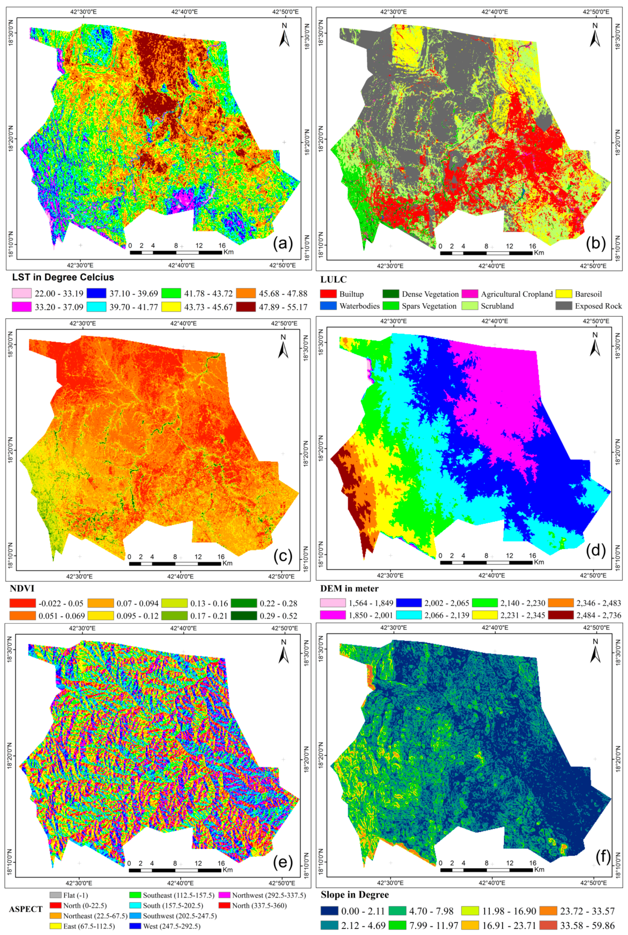
The LST was strong in north and east and low in west and south, showing a relatively steady decline from northeast to southwest. Additionally, the LST created a high-value area in downtown Abha-Khamis-Mushyet cities and other land-intensive building areas, showing a daily high-temperature (heat island) geographical phenomenon. In the Eastern part of the study area, i.e., the Khamis-Mushyet town, the LST formed a high-value area whereas, in the western part, i.e., Abha City, LST was low-value. The combination of elevation, NDVI, and LULC data were used to overlay analysis, which showed that the trend was mainly attributable to the cumulative effects of LULC, NDVI, and elevation. Moreover, the integration of high-resolution thermal maps revealed high-temperature zones distinct from the city’s typical urban thermal environment. Apart from this, the highest LST was noted in the northern study area, due to exposed rocky area.

4.2. Relationship between LST and LULC

LST was ranked as follows, among different types of LULC-exposed rock > built-up land > bare soil > scrubland > agricultural cropland > sparse vegetation > dense water bodies (Table 2). LST of sparse vegetation and built-up land was high, including its standard deviation. Generally, the LST of built-up, bare soil, and agricultural cropland with high a anthropogenic influence was higher than other LULC classes; the LST of the water body and, dense vegetation that had low anthropogenic influence was significantly low. Hence, LULC classes should be planned realistically, and the effect of coolness should be encouraged by water and vegetation. Table 2 presents the results of the post-hoc test related to the LST and NDVI variations between various classes of LULC in the study area.
Agricultural cropland was predominantly dry land with limited plant density, while sparse vegetation was mostly dry soil, Acacia woodlands, i.e., Acacia origena and A. gerrardii and low vegetation coverage. Agricultural cropland and sparse vegetation coverage showed only a substantial difference in surface emissivity, with no significant difference in LSTs; these influences could also be seen in the mean NDVI value of agricultural land and sparse vegetation. Influenced by differing heat flux, thermal conductivity and thermal radiation properties, the surface temperature of dense vegetation, water bodies, exposed and built-up rock showed significant variations, indicating that the various forms of LULC contributed significantly to the local thermal environment (Figure 3). Analysis of surface temperature distribution over built-up land revealed that high impermeable surface densities and low vegetation cover led to adverse shifts in the study area’s thermal environment.

4.3. LST and NDVI Relationship

Characteristics LST and NDVI Distribution

The statistics of surface temperature and NDVI by LU/LC types were obtained by superimposing LULC with surface temperature, and NDVI. Figure 4a,c infer that the NDVI and LST displayed patterns of inverse spatial distribution. The LST showed opposite patterns in two separate ways, with the corresponding NDVI. The histogram profile of NDVI and LST over different LULC is shown in Figure 5. The surface temperature in Abha-Khamis-Mushyet twin cities developed a high-value area, showing an urban thermal pattern phenomenon that is exceptional for exposed rocky areas; further, the low-value NDVI zones in this region exhibited a small impact. The high LST peaks were related to the low NDVI value; meanwhile, the high NDVI peak areas, corresponded exactly to the low LST value.
On the contrary, the low LST and NDVI water body indicated its effective cooling effect. Compared to the built-up areas, the vegetation has “shown a significantly lower surface temperature, as dense vegetation can reduce the heat stored and surface structures by transpiration and minimize the soil” background. The LST of water bodies appeared to be low because the water slowly warmed up during the day, “possessing high thermal inertia and convection and turbulence” (for example, wave action). The water temperature was generally consistent with a vegetable coverage of about zero, and the water LST correlated positively with NDVI [77]. Meanwhile, the main part of the bare soil and the exposed rocky area was the absence of vegetation coverage.
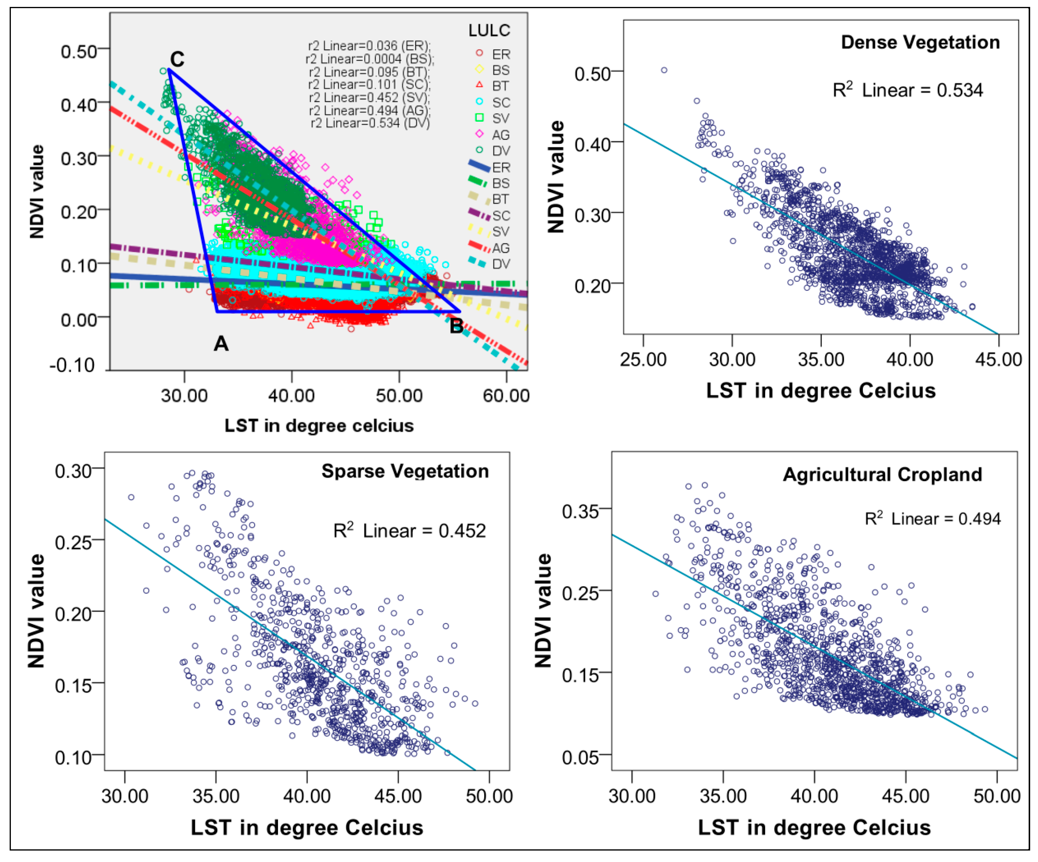
Consequently, in the discussion of the linear coefficient relationship between NDVI and LST, between various LULC, the bare soil, exposed rock area, and water bodies were not taken into account. Figure 6 shows the linear regression coefficient between LST and NDVI for the LULC class as a whole, dense vegetation, agricultural land, and sparse vegetation. The most significant “coefficient of regression between LST and NDVI values found in dense vegetation (R2 = −0.534) tailed agricultural cropland vegetation (R2 = −0.494) and sparse vegetation (R2 = −0.452)”. In dense vegetation, agricultural croplands and sparse vegetation, with high to moderate correlation was observed between NDVI with surface temperature, which could use linear regression to simulate summer surface temperature, if the NDVI values were known (Figure 6). The surface temperature could, therefore, be precise and reasonably simulated using the NDVI value during the summer or lower precipitation periods. Figure 4 illustrates that the LSTs of the various LULC classes had a negative linear regression coefficient with the NDVI value. In the linear regression coefficient, the values were ranked as follows—dense vegetation > agricultural cropland > sparse vegetation > scrubland, representing that the surface temperature of the dense vegetation decreased rapidly with increased NDVI value, followed by agricultural cropland and sparse vegetation, whereas the scrubland surface temperature declined slower rate. Thus, the surface temperature of dense and sparse vegetation and agricultural cropland was more influenced by vegetation cover than the scrubland and built-up land, and its cooling impact was more apparent than that of other types of LULC. Consequently, an adequate increase in green areas in urban lands improved the thermal environment in the city.

4.4. Spatial Structure of LST and LULC Relationship

Due to the unusual occurrence of single land use, the LST-NDVI relationship should be studied in a spatial combination of various forms of LULC. In Figure 6, the LST–NDVI feature space represents a unique triangle shape with an obtuse-angled ABC. A represents a low LST water body and a relatively negative NDVI value; B represents bare soils, exposed rock and built-up with high-LST and low-NDVI value; and C represents dense vegetation with the lowest-LST value and highest-NDVI value. In Figure 6, the different types coincided with each other in the LST–NDVI feature space; built-up, mostly mixed with exposed rock and bare soil had high evaporation and low moisture content; sparse vegetation was spread in the transitional zone between the agricultural cropland and dense vegetation, with high vegetation cover, relatively abundant soil moisture and low evapotranspiration. The dense vegetation’s main distribution was localized mainly and followed Wadi from north-east to south-west (Figure 7).

4.5. Relationship between LST and Topographical Parameters

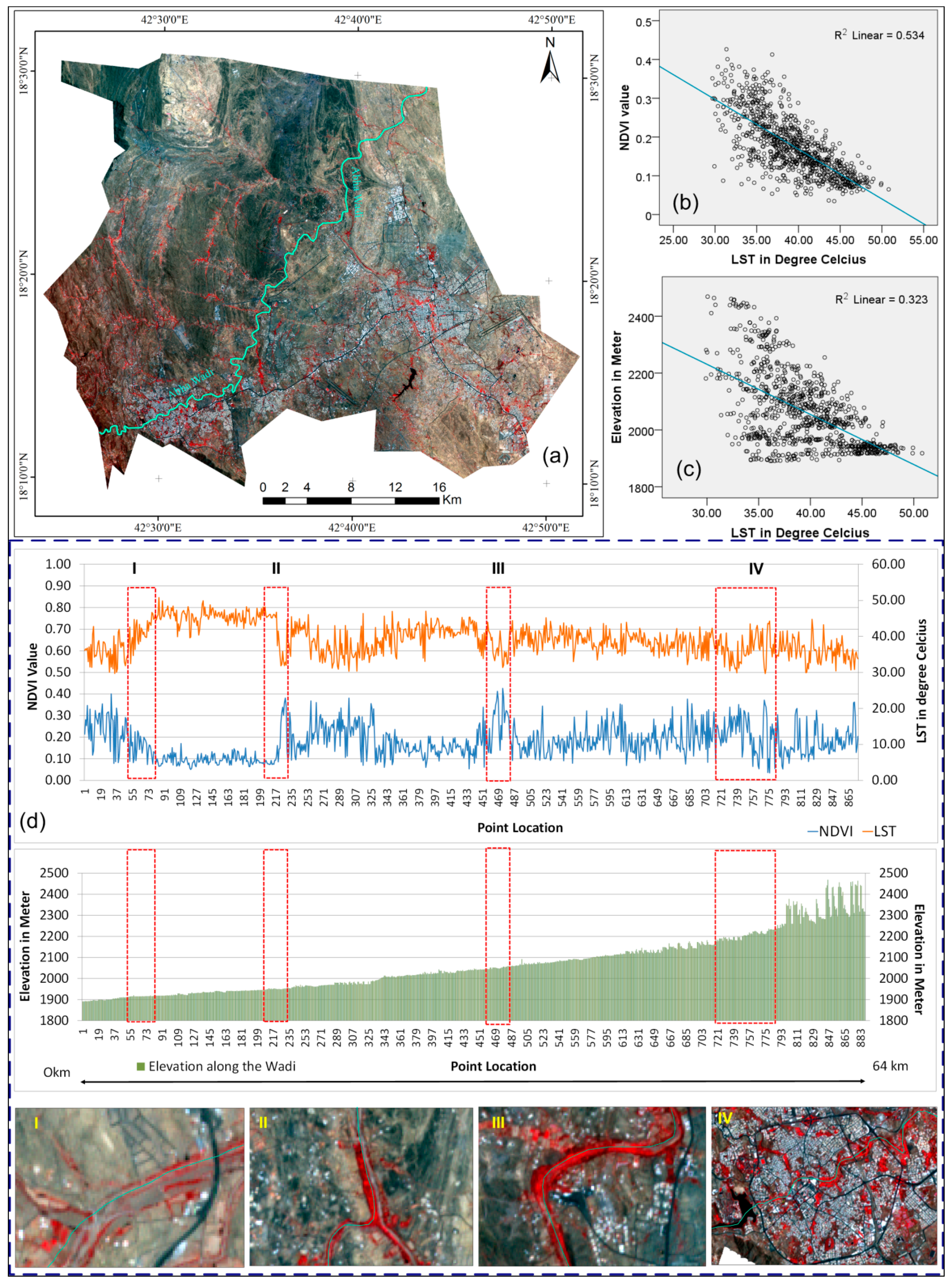
The topographical impacts on surface temperature were examined in-depth, in terms of elevation, slope, and aspect with a basic understanding of surface temperature change patterns, as shown in Figure 4 and Figure 6. The surface temperature and altitude spatial distribution exhibited an inverse pattern. With increasing altitude, the surface temperature gradually decreased. Topographical distribution alternated between the valleys and hills in east-west and northeast–southwest directions. Accordingly, the high-value peaks and low-value valleys of the surface temperature were distributed alternately. Moreover, the surface temperature had a notably vertical variation rule in the region, with a relatively high altitude difference. Taking Alsouda mountain (located in western part; elevation 2730 m MSL) and Khamish-Mushayet city (located in the eastern part) as examples, Figure 4d shows a low altitude in the Khamish-Mushayet area (Elevation 2000 m MSL), where there is a high surface temperature value. Figure 7 illustrates that the surface temperature of high hills gradually declined with the increase in elevation.

4.5.1. Effect of Elevation on the LST

To determine the effect of elevation on the surface temperature over different LULC, the relationship between the LST and the elevation was investigated through zonal statistical analysis, using ArcGIS software (Table 3) and scatter plot (Figure 7c), which showed the effect of elevation on the LST, similar to the effect of elevation in the air temperature [78]. Table 3 shows the statistical analysis LST over the various LULC, at the classified elevation zone. The elevation effect on the LST was clearly expressed over various LULC. The built-up land, the mean NDVI and LST at the elevation of 1564–2000 m was 0.061 and 46.14 °C, respectively, whereas at the elevation of 2501–2736 m, NDVI increase gradually and LST decrease gradually to 0.123 and 39.29 °C. A similar pattern of a gradual decrease in LST was found in the overall LULC classes because of the holistic impacts from surface type, solar radiation, meteorological conditions, the thermal property of the underlying materials, etc. The major gradual decrease in inclination was found over the densely vegetated area. However, statistical analysis of LST and elevation revealed that with a rise in elevation, the overall trend of LST declined. Due to the strong interactive effects from different factors, the relationship was thus more complex.

4.5.2. Effect of Aspect on the LST

In mountainous regions, the slope and aspect are known to affect radiation conditions. Different aspects alter the conditions of sun shading and cause the thermal interactions of the land surfaces. To strengthen the knowledge of the topographic effect on LST, the changing LST trends were assessed in eight cardinal directions “(North (0–22.5 and 337.5–360), Northeast (22.5–67.5), East (67.5–112.5), Southeast (112.5–157.5), South (157.5–202.5), Southwest (202.5–247.5), West (247.5–292.5), and Northwest (292.5–337.5)” derived from the aspects (Figure 4e). Zonal statistics of the elevation zone was performed on each direction using NDVI and LST values to obtain the corresponding statistics. As depicted in Table 4, analysis findings from the variances in the cardinal directions was the highest in the east (67.5–112.5) and the southeast (112.5–157.5), at an elevation of 1564–2000 m, with a temperature of 47.05 °C and 47.11 °C, respectively. The statistical analysis between the LST and the aspect demonstrated the overall trend of the surface temperature going down with increasing elevation in all eight cardinal directions.
Moreover, the highest LST value found in the east (67.5–112.5) and the southeast (112.5–157.5) at an elevation of 2501–2736 m were 39.81 °C and 40.69 °C, respectively. The highest LST found over the east (67.5–112.5) and southeast (112.5–157.5) cardinal direction were attributed to variations in local radiative and weather conditions. Therefore, the scattering distribution between the LST and the elevation for each direction was substantially reduced due to the different aspects. Whereas, the lowest LST found in the southwest (202.5–247.5) and the west (247.5–292.5), at an elevation of 1564–2000 m was 45.23 °C and 45.03 °C, respectively. Moreover, the lowest LST found in the southwest (202.5–247.5) and the west (247.5–292.5) at an elevation of 2501–2736 m was 35.93 °C and 35.84 °C, respectively. The statistical analysis of aspect with NDVI also drew some valuable finding. The lower NDVI value was found in the east (67.5–112.5) and the southeast (112.5–157.5), at an elevation of 2501–2736 m. This could be attributed to higher temperatures and shifts in precipitation trends over the past three decades, which could account for the observed rise in junipers’ drought stress at these altitudes [79]. These situations seem to suggest that the influence of aspect difference on LST should be a strong feature for various locations with different seasons. As for the process, the difference in surface solar radiation in each cardinal direction would cause directional changes. Slopes facing the sun receive more solar radiation, allowing faster heating than the slopes away from sunlight. Additionally, the LST of slopes facing the sun was higher than the LST of slopes faced away from the sun.

4.5.3. Effect of Slope on the LST

Besides the aspect impact, the slope factor also significantly regulated the quantity of direct radiation exposure that is commonly more global radiation percentage than the sky diffuse radiation, through both the angle between the normal slope and the solar beam. This might be why incoming solar radiation on earth’s surface was quite susceptible to the slope and influenced the heating process of the surface. The image acquisition time for the Abha-Khamish-Mushyet area was 10:49:09 a.m., and the research area’s mountain path was southeast for the sunlit slope and the shady north-west slope (Figure 4f). In the analysis, the average sunlit slope LST was 2.32 °C above the shady slope. To analyze the slope impact separately, we categorized the local solar zenith angle into five zones, as per the natural break method, and the zonal statistics of the elevation zone was performed at each slope range, using the NDVI and LST values, to obtain the corresponding statistics (Table 5). A specific phenomenon could be identified from the LST value presented in Table 5, which showed that there was a significant declining trend with a higher slope angle. Variations in LST values at various angles could range from 1564–2000 to 2501–2736, approximately 3–4 °C, indicating an important effect of the surface slope on LST. Though under different slope conditions, the frequency of the influence changed and it was linked to the atmospheric impacts and types of LULC.

4.5.4. Effect of Vegetation on the LST

It was evident that changes in the LST values were highly linked with changes in the topographical conditions. However, the relationship was not unique, and the vegetation often played a crucial role in the changes to the LST. Sandholt et al. [80] reported that the vegetation not only regulated the LST through the surface energy balance, but also affected the sensor’s visible bare soil and vegetation coverage and changes in the radiative temperature between the vegetation canopy and the soil influence on the LST. In addition, the thermal characteristics of the surface were also partially affected by the vegetation conditions. For example, the LST assessment of the study area was chosen to explore the impacts to examine the LST variations under different vegetation conditions. As seen in Table 3 and Table 4, NDVI was used as an indicator of vegetation and categorized into different ranges. In most circumstances, the areas with lower NDVI value could be considered as the bare surfaces (Figure 4c). Though a declining trend could be observed with the increase in the NDVI value, and this trend indicated the vegetation’s thermal impacts, including evaporative control, thermal properties, and surface radiative balance. With vegetation canopy increases, the LST decreased within a relatively low-temperature range. This decrease might be reflected in part from the triangle space investigated in many studies between LST and NDVI.

4.6. Spatial Characteristics of NDVI and LST Distribution

Examining surface temperature patterns, transect (profile) was drawn across the image, i.e., north-east and south-west, along the Abha Wadi shown in Figure 7. This transect was made to observe a relationship in LST–NDVI-Elevation. Such transects enabled us to understand the factors that influence the city’s thermal environment, as well as the role of vegetation with topographical variation. From the spatial profile of transects, it could be seen that there were high peaks LST value (box I) related to a low ‘peaks’ of the NDVI. Meanwhile, the zone highlighted with boxes (II and III) depicted the high peaks of NDVI value, which corresponded exactly to the low LST ‘valley’. Two boxes in the Abha Wadi profile, i.e., I and IV, were characterized by comparatively low NDVI and LST. The low LST and NDVI suggest its strong cooling effect, as seen in box IV. In addition, in the spatial profile of transects, LST correlated negatively with elevation and moderately with the low linear coefficient of R2 = −0.323. In contrast, LST was negatively correlated with the NDVI and showed a high linear coefficient of R2 = −0.534.

5. Discussion

In this study, LSE retrieved from NDVI-derived emissivity method and its integration into the TES algorithm was applied to ASTER multi-spectral thermal data to accurately estimate LST. In the TES algorithm, surface emissivities were determined based on TIR image data alone, which led to scaling errors in the estimation of emissivity in heterogeneous surfaces, especially in the vegetated areas. The TES algorithm problem MMD threshold was where the target emissivities were close to the threshold value of 0.03. It related to the scaling errors that ultimately resulted in a scaling-value jump that induced discontinuity in the image of a transition from bare soil to the vegetation. Due to variations in the scaling of high-low MMD emissivity spectra in TES, it was appropriate to use ASTER’s VNIR data to estimate vegetation proportion cover and surface emissivity, irrespective of TIR data. The results showed that emissivity derived from the NDVI method was more reliant on the upwelling, downwelling, and transmittance and would provide the best results [74]. The main strength of emissivity derived from the NDVI algorithms was the potential within the algorithms to incorporate atmospheric correction [81].
There are various advantages and disadvantages in contrasting the emissivity approach derived from NDVI with the TES methods. The TES algorithm provided a significant accuracy for LSE. However, the TES accuracy for surfaces with low MMD values was expected to decrease, as was the case with vegetated areas [74]. The results from the NDVI approaches were predicted to be marginally better in this case of LSE. Nevertheless, the emissivity-derived NDVI approach did not extend to surfaces with negative NDVI values, i.e., water, the emissivity spectra were also well-known for all surfaces. The efficiency of the TES method over low MMD surfaces need further studying and validation, besides adapting the NDVI method to rock covers. The ability to retrieve LST, together with LSE, was one advantage of the emissivity derived from the NDVI approach [74,81]. The emissivity method derived from NDVI offered improvements in surface emissivity prediction from visible and NIR data. This point should be considered when evaluating the NDVI-derived emissivity method; it referred to the estimation of the vegetation proportion cover from NDVI values (Equation (2)), according to Carlson and Ripley [82]. This was a simple method of estimating the vegetation proportion cover and was sufficiently accurate for using the NDVI method. Furthermore, a multi-spectral analysis by endmembers might result in an improvement in the estimation of vegetation proportion; although the principal source of error in the NDVI methodology is the selection of soil emissivity.
An increase in vegetation areas is the main option discussed for local climate mitigation [53]. Vegetation in urban areas governs climate mainly through shading [54], carbon dioxide sequestration [55], and evapotranspiration [56]. The mitigation potential of urban vegetation requires additional research because vegetation and local climate are strongly associated, and local plant species should be preferred as a strong mitigation option; however, exotic trees are common in the urban context. When vegetation becomes denser, there is a general decreasing trend in the LST (exhibited by the increase in NDVI). The dense vegetation canopy effectively prevents incident solar radiation and improves the evaporative cooling effect of vegetation, which prevents a rise in surface temperature [23,57,58,59]. Therefore, the surface temperature decreases with the increase in vegetation cover. The terrain impact evaluation on the LST indicates that the change in temperature pattern shows significant variations with respect to the main factors associated with elevation, vegetation cover, slope and aspect, consistent with He et al. [57] findings. The general geographic phenomenon was observed for LST spatio-temporal variation at different seasons or different latitudinal locations. The seasonal MODIS LST correlation analysis [51,78] not only confirmed the important impact of topography and land cover on LST variation but also offered insights into the topography effect on LST by quantitatively examining temperature drop variability concerning various factors, slope, aspect, vegetation, and solar radiation.
The urban thermal effect of the built-up and densely populated area was notable in Abha-Khamis-Mushayet cities during the summer season (June). As such, apart from those induced by the classical urban thermal effect, several zones of high LST with various sizes and shapes were noticed in the study area’s northern and central portion. From the LST distribution, the highest LST of more than 53 °C was observed where no construction was found. Abnormal regions of high LST were located mostly in the northern and central sections of the study region, with no vegetation cover and exposed rocky areas (Figure 4b). Bare soil contributed to low vegetation cover [83], surface water infiltration, loss of water [84], human intrusion, and degradation causes extreme soil erosion [20], resulting in exposed rock exposure and rocky desertification [85]. Therefore, surface substances’ specific heat capacity and thermal inertia were low. Consequently, the LST area grew rapidly during the day and was higher in the surrounding area, producing an abnormal zone of high LST. Thereby, the LST of the exposed rocky areas characterized not only by the classical urban thermal effect but also the abnormal zone of high LST, exacerbated by the desertification in the rocky area. In future studies, LST could be used as a critical element and index to examine and assess the degree of desertification in rocky areas.
Twin cities Abha-Khamis-Mushayet have prominent mountain features, with mountains representing a more significant portion of the study area. Figure 5D indicates a tilting of the terrain from southwest to northeast, while a decrease in LST from northeast to southwest stretched along the mountains, suggesting a dominant role in the LST of the region by altitude, and there was a negative correlation between LST and elevation in the quantitative relation. Two principal factors were responsible for this pattern. (1) Surface temperature influenced by air-temperature, was also decreased with height. (2) In semi-arid mountainous regions, Abha-Khamis-Mushayet twin cities, the vegetation cover on the southwest side was relatively good compared to the north and the northeast. So the solar radiation that the ground surface received was often spread in latent heat, and low LST. In the meantime, the intensity and length of solar radiation varied in various slope directions. In this analysis, the LST also differed across multiple slope directions, consistent with the Wen et al. [86] findings. Different types of LULC show different thermal conductivity, thermal capacity, roughness, and albedo, resulting in LST variations. In the analysis, the LSTs of different LULC types differed in the same direction at the same elevation. In overview, the LST in this present study area was affected by altitude, slope aspect, and LULC type, in which elevation and vegetation played a key role in the overall LST pattern.
Current literature on the LST–NDVI relationship varied substantially in combinations of different LULC classes (Table 6). In this research, the LST and NDVI scatter plot diagram showed an obtuse-angled triangle distribution in combinations of different LULC classes, consistent with the Zhou et al. [87] findings.
Still, it varied from what was found by other researchers, due to variations between quantitative and qualitative analyses or variations in soil backgrounds and the sensor used in the studied area. The LST–NDVI feature space showed a unique ABC obtuse-angled triangle shape an overall showed a negative linear correlation. Clearly, A characterized a water body with low-LST and somewhat negative NDVI value; B characterized bare soils, exposed rock, and built-up with high-LST and low NDVI value; and C characterized dense vegetation with the lowest LST value and the highest NDVI value, which was compatible with the findings of Zhou et al. [87]. Nevertheless, it should be noted that the analysis still had limitations. Soil moisture should be a very significant factor affecting LST’s evolution. Several studies showed their indirect relationship and established methods to infer soil surface moisture, based on LST variation [28,44,76]. Consequently, in future research, the surface moisture effect should be known to some degree.

6. Conclusions

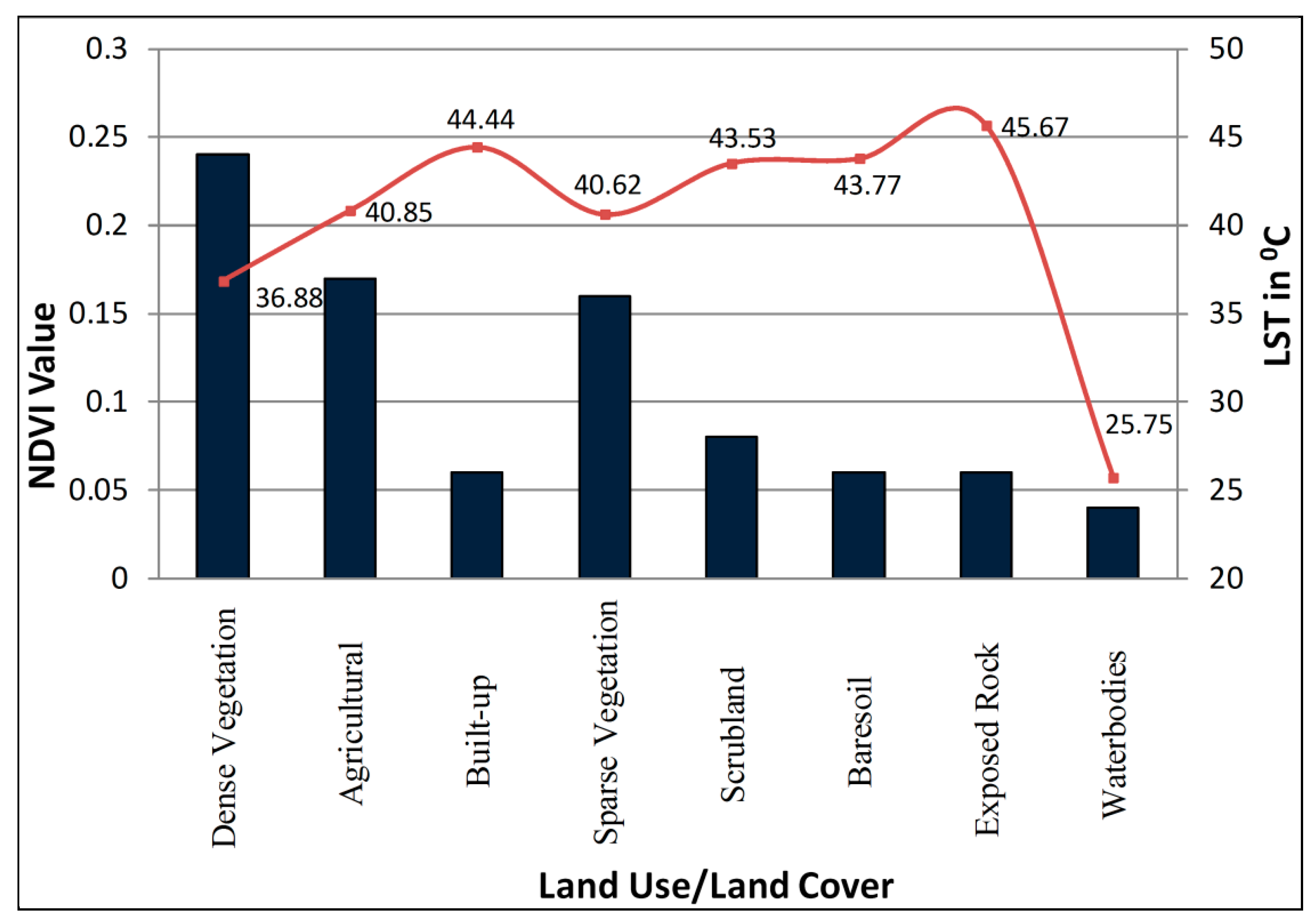
In the present study, LSE was retrieved from the proportion of vegetation cover in conjunction with NDVI and integrated into the TES algorithm to derive LST from ASTER data. The spatial distribution patterns of LST and factors of influence in the semi-arid mountain cities of Abha-Khamish-Mushayet were summarized by combining LULC classes and NDVI with DEM data. The LST variations between various LULC classes were then investigated and the characteristics of the distribution of NDVI and LST in the study area and their quantitative relationship were discussed. The main contributions of this research were described (1) retrieving LST from the proportion of vegetation cover in conjunction with NDVI integrated into the TES algorithm and comparing the estimated satellite surface temperature values with ground-based measurements (in-situ), which was consistent with the actual value. Influenced by topographical parameters, i.e., elevation, slope, aspect, and underlying types of LULC, LST exhibited an overall decreasing trend from northeast to southwest and stretched across the extent of the mountain, suggesting a role of LST by altitude. The imaging time, i.e., summer, abnormal regions of high-temperature were located mainly in the northern and central sections of the study region, with no vegetation cover and exposed rocky areas. Bare soil contributed to low vegetation cover, surface water infiltration, loss of water, human intrusion, and degradation caused extreme soil erosion, resulting in exposed rock exposure and rocky desertification. Therefore, surface substances’ specific heat capacity and thermal inertia were low. Consequently, the LST area grew rapidly during the day and was higher in the surrounding area, producing an abnormal zone of high LST. (2) Several comparative analysis indicated that the difference in LST was important among most types of LULC; the exposed rock area exhabited the highest mean LST of 45.67 °C, followed by built-up land of 44.44 °C, and water bodies and dense vegetation exhibited the lowest LST of 25.75 °C and 36.88 °C, respectively. LSTs were ranked as follows, among different types of land use/land cover: exposed rock > built-up > bare soil > scrubland > agricultural > sparse vegetation > dense water bodies. Generally, the LST of built-up, bare soil, and agricultural cropland with high anthropogenic influence intensity was higher than other LULC classes; the LST of the water body and, dense vegetation, which had low anthropogenic influence intensity, and was significantly low. Hence, LULC classes should be planned realistically, and the effect of coolness should be encouraged by water and vegetation. (3) For the LULC type, water bodies, bare soil, and exposed rocky area were not considered in the discussion on the linear coefficient relationship between NDVI and LST, as it had a nonlinear relationship. The most significant “coefficient of regression between the LST and NDVI values were found in dense vegetation (R2 = −0.534), tailed agricultural cropland vegetation (R2 = −0.494), sparse vegetation (R2 = −0.452)”. In dense vegetation, agricultural croplands and sparse vegetation, with a high to moderate correlation was observed between NDVI with surface temperature, which could use linear regression to simulate summer surface temperature, if the NDVI values were known. The surface temperature could, therefore, be precise and reasonably simulated using the NDVI value during the summer or lower precipitation periods. (4) The LST–NDVI feature space showed a unique ABC obtuse-angled triangle shape. Conclusively, A represented a water body with low LST and relatively negative NDVI value; B represented bare soils, exposed rock, and built-up with high LST and low NDVI value; and C represented dense vegetation with the lowest LST value and the highest corresponding NDVI value. (5) The vegetation cover on the southwest side was relatively good compared to the north and the northeast. So the solar radiation that the ground surface received often spreads in latent heat, and low LST. In the meantime, the solar radiation length and intensity varied in various directions of the slope. The LST also varied in different slope directions. Different types of LULC had varied thermal conductivity, thermal capacity, roughness, and albedo, resulting in LST variations. In the analysis, the LSTs of different LULC types differed in the same direction at the same elevation. The LST was affected by elevation, slope aspect, and LULC class, in which elevation and vegetation played a key role in the overall LST pattern. This study offers a framework for land-use planning and environmental protection in urban mountainous areas.

Author Contributions

Conceptualization, A.A.B. and J.M.; Data curation, J.M.; Formal analysis, A.A.B., C.K.S. and H.T.H.; Investigation, J.M. and S.A.; Methodology, J.M. and H.T.H.; Project administration, A.A.B. and J.M.; Resources, S.A., C.K.S. and H.T.H.; Software, H.T.H.; Supervision, S.A.; Validation, A.A.B. and S.A.; Writing–original draft, A.A.B. and J.M.; Writing–review & editing, C.K.S. All authors have read and agreed to the published version of the manuscript.

Funding

Funding for this research was given under award numbers R.G.P2/75/41 by the Deanship of Scientific Research; King Khalid University, Ministry of Education, Kingdom of Saudi Arabia.

Acknowledgments

Authors thankfully acknowledge the Deanship of Scientific Research for proving administrative and financial supports, and the NASAUSGS personnel at the land DAAC for providing the latest ASTER-Terra satellite image.

Conflicts of Interest

The authors declare no conflict of interest.

References

  1. Van De Kerchove, R.; Lhermitte, S.; Veraverbeke, S.; Goossens, R. Spatio-temporal variability in remotely sensed land surface temperature, and its relationship with physiographic variables in the Russian Altay Mountains. Int. J. Appl. Earth Obs. Geoinf. 2012. [Google Scholar] [CrossRef] [Green Version]
  2. Aguilar, C.; Herrero, J.; Polo, M.J. Topographic effects on solar radiation distribution in mountainous watersheds and their influence on reference evapotranspiration estimates at watershed scale. Hydrol. Earth Syst. Sci. 2010. [Google Scholar] [CrossRef] [Green Version]
  3. Ivanov, V.Y.; Bras, R.L.; Vivoni, E.R. Vegetation-hydrology dynamics in complex terrain of semiarid areas: A mechanistic approach to modeling dynamic feedbacks. Water Resour. Res. 2008. [Google Scholar] [CrossRef] [Green Version]
  4. Rolland, C. Spatial and seasonal variations of air temperature lapse rates in alpine regions. J. Clim. 2003. [Google Scholar] [CrossRef] [Green Version]
  5. Dash, P.; Göttsche, F.M.; Olesen, F.S.; Fischer, H. Land surface temperature and emissivity estimation from passive sensor data: Theory and practice-current trends. Int. J. Remote Sens. 2002. [Google Scholar] [CrossRef]
  6. Kaufman, Y.J.; Wald, A.E.; Remer, L.A.; Gao, B.C.; Li, R.R.; Flynn, L. MODIS 2.1-μm channel—Correlation with visible reflectance for use in remote sensing of aerosol. IEEE Trans. Geosci. Remote Sens. 1997. [Google Scholar] [CrossRef]
  7. Gillespie, A.; Rokugawa, S.; Matsunaga, T.; Cothern, J.S.; Hook, S.; Kahle, A.B. A temperature and emissivity separation algorithm for advanced spaceborne thermal emission and reflection radiometer (ASTER) images. IEEE Trans. Geosci. Remote Sens. 1998. [Google Scholar] [CrossRef]
  8. Guillevic, P.; Göttsche, F.; Nickeson, J.; Hulley, G.; Ghent, D.; Yu, Y.; Trigo, I.; Hook, S.; Sobrino, J.A.; Remedios, J.; et al. Land surface temperature product validation best practice protocol version 1.1. Best Pract. Satell.-Deriv. Land Prod. Valid. 2018. [Google Scholar] [CrossRef]
  9. McMillin, L.M. Estimation of sea surface temperatures from two infrared window measurements with different absorption. J. Geophys. Res. 1975. [Google Scholar] [CrossRef]
  10. Wan, Z. A generalized split-window algorithm for retrieving land-surface temperature from space. IEEE Trans. Geosci. Remote Sens. 1996. [Google Scholar] [CrossRef] [Green Version]
  11. Prata, A.J.; Casellescoll, C.V.; Sobrino, J.A.; Ottle, C. Thermal remote sensing of land surface temperature from satellites: Current status and future prospects. Remote Sens. Rev. 1995. [Google Scholar] [CrossRef]
  12. Li, Z.L.; Becker, F. Feasibility of land surface temperature and emissivity determination from AVHRR data. Remote Sens. Environ. 1993. [Google Scholar] [CrossRef]
  13. Hook, S.J.; Gabell, A.R.; Green, A.A.; Kealy, P.S. A comparison of techniques for extracting emissivity information from thermal infrared data for geologic studies. Remote Sens. Environ. 1992. [Google Scholar] [CrossRef]
  14. Kealy, P.S.; Hook, S.J. Separating temperature and emissivity in thermal infrared multispectral scanner data: Implications for recovering land surface temperatures. IEEE Trans. Geosci. Remote Sens. 1993. [Google Scholar] [CrossRef]
  15. Valor, E.; Caselles, V. Mapping land surface emissivity from NDVI: Application to European, African, and South American areas. Remote Sens. Environ. 1996. [Google Scholar] [CrossRef]
  16. Vázquez, D.P.; Reyes, F.J.O.; Arboledas, L.A. A comparative study of algorithms for estimating land surface temperature from AVHRR data. Remote Sens. Environ. 1997. [Google Scholar] [CrossRef]
  17. Qin, Z.; Karnieli, A.; Berliner, P. A mono-window algorithm for retrieving land surface temperature from Landsat TM data and its application to the Israel-Egypt border region. Int. J. Remote Sens. 2001. [Google Scholar] [CrossRef]
  18. Jiménez-Munoz, J.C.; Sobrino, J.A. A generalized single-channel method for retrieving land surface temperature from remote sensing data. J. Geophys. Res. Atmos. 2003. [Google Scholar] [CrossRef] [Green Version]
  19. Baldridge, A.M.; Hook, S.J.; Grove, C.I.; Rivera, G. The ASTER spectral library version 2.0. Remote Sens. Environ. 2009. [Google Scholar] [CrossRef]
  20. Mallick, J.; Rahman, A.; Singh, C.K. Modeling urban heat islands in heterogeneous land surface and its correlation with impervious surface area by using night-time ASTER satellite data in highly urbanizing city, Delhi-India. Adv. Space Res. 2013. [Google Scholar] [CrossRef]
  21. Li, Z.L.; Wu, H.; Wang, N.; Qiu, S.; Sobrino, J.A.; Wan, Z.; Tang, B.H.; Yan, G. Land surface emissivity retrieval from satellite data. Int. J. Remote Sens. 2013. [Google Scholar] [CrossRef]
  22. Vostikolaei, F.S.; Akhoondzadeh, M. A comparison of four methods for extracting land surface emissivity and temperature in the thermal infrared hyperspectral data. Earth Obs. Geomat. Eng. 2018, 2, 56–63. [Google Scholar] [CrossRef]
  23. Mallick, J. Land characterization analysis of surface temperature of semi-arid mountainous city Abha, Saudi Arabia using remote sensing and GIS. J. Geogr. Inf. Syst. 2014. [Google Scholar] [CrossRef] [Green Version]
  24. El-Nahry, A.H.; Rashash, A. Impact of industrial areas on surface temperature using thermal infrared remote sensing and GIS techniques: A case study of Jubail City, KSA. In Proceedings of the 8th National GIS Symposium in Saudi Arabia, Dammam, Saudi Arabia, 8 June 2013. [Google Scholar]
  25. Rashash, A.A.; Mohammed, E.S. Impact of industrial activities on land surface temperature using remote sensing and GIS techniques—A case study in Jubail, Saudi Arabia. J. Geogr. Nat. Disasters 2016. [Google Scholar] [CrossRef] [Green Version]
  26. Mujabar, S.; Rao, V. Estimation and analysis of land surface temperature of Jubail Industrial City, Saudi Arabia, by using remote sensing and GIS technologies. Arab. J. Geosci. 2018. [Google Scholar] [CrossRef]
  27. Mujabar, P.S. Spatial-temporal variation of land surface temperature of Jubail Industrial City, Saudi Arabia due to seasonal effect by using Thermal Infrared Remote Sensor (TIRS) satellite data. J. Afr. Earth Sci. 2019. [Google Scholar] [CrossRef]
  28. Berg, A.; Lintner, B.R.; Findell, K.L.; Malyshev, S.; Loikith, P.C.; Gentine, P. Impact of soil moisture-atmosphere interactions on surface temperature distribution. J. Clim. 2014. [Google Scholar] [CrossRef] [Green Version]
  29. Li, Z.L.; Tang, B.H.; Wu, H.; Ren, H.; Yan, G.; Wan, Z.; Trigo, I.F.; Sobrino, J.A. Satellite-derived land surface temperature: Current status and perspectives. Remote Sens. Environ. 2013. [Google Scholar] [CrossRef] [Green Version]
  30. Dickinson, R.E. Satellite systems and models for future climate change. In Future Climates of the World: A Modelling Perspective, 16th ed.; Henderson-Sellers, A., Ed.; World Survey of Climatology Elsevier: Amsterdam, The Netherlands, 1994; p. 27. [Google Scholar]
  31. Becker, F.; Li, Z.L. Surface temperature and emissivity at various scales: Definition, measurement and related problems. Remote Sens. Rev. 1995. [Google Scholar] [CrossRef]
  32. Zareie, S.; Khosravi, H.; Nasiri, A.; Dastorani, M. Using Landsat Thematic Mapper (TM) sensor to detect change in land surface temperature in relation to land use change in Yazd, Iran. Solid Earth 2016. [Google Scholar] [CrossRef] [Green Version]
  33. Vlassova, L.; Perez-Cabello, F.; Nieto, H.; Martín, P.; Riaño, D.; Riva, J.D. Assessment of methods for land surface temperature retrieval from Landsat-5 TM images applicable to multiscale tree-grass ecosystem modeling. Remote Sens. 2014, 6, 4345–4368. [Google Scholar] [CrossRef] [Green Version]
  34. Kustas, W.; Anderson, M. Advances in thermal infrared remote sensing for land surface modeling. Agric. For. Meteorol. 2009. [Google Scholar] [CrossRef]
  35. Quattrochi, D.A.; Luvall, J.C. Thermal Remote Sensing in Land Surface Processing; CRC Press: Boca Raton, FL, USA, 2004. [Google Scholar]
  36. Jia, L.; Menenti, M.; Su, Z.; Li, Z.-L.; Djepa, V.; Wang, J. Modeling sensible heat flux using estimates of soil and vegetation temperatures: The HEIFE and IMGRASS experiments. In Remote Sensing and Climate Modeling: Synergies and Limitations; Springer: Dordrecht, The Netherlands, 2001. [Google Scholar]
  37. Kalma, J.D.; McVicar, T.R.; McCabe, M.F. Estimating land surface evaporation: A review of methods using remotely sensed surface temperature data. Surv. Geophys. 2008. [Google Scholar] [CrossRef]
  38. Linh, N.T.; Huy, T.Q.; Jungwon, H.; Dongyeob, H. Land Surface temperatures of industrial complexes in Jeonnam using Landsat 7 ETM+ satellite images. J. KRSA 2015, 15, 87–95. [Google Scholar]
  39. Xu, T.; Bateni, S.M.; Margulis, S.A.; Song, L.; Liu, S.; Xu, Z. Partitioning evapotranspiration into soil evaporation and canopy transpiration via a two-source variational data assimilation system. J. Hydrometeorol. 2016. [Google Scholar] [CrossRef]
  40. Peng, J.; Loew, A.; Chen, X.; Ma, Y.; Su, Z. Comparison of satellite-based evapotranspiration estimates over the Tibetan Plateau. Hydrol. Earth Syst. Sci. 2016. [Google Scholar] [CrossRef] [Green Version]
  41. Anderson, M.C.; Allen, R.G.; Morse, A.; Kustas, W.P. Use of Landsat thermal imagery in monitoring evapotranspiration and managing water resources. Remote Sens. Environ. 2012. [Google Scholar] [CrossRef]
  42. Li, Z.L.; Tang, R.; Wan, Z.; Bi, Y.; Zhou, C.; Tang, B.; Yan, G.; Zhang, X. A review of current methodologies for regional Evapotranspiration estimation from remotely sensed data. Sensors 2009, 9, 3801–3853. [Google Scholar] [CrossRef] [Green Version]
  43. Amiri, R.; Weng, Q.; Alimohammadi, A.; Alavipanah, S.K. Spatial–temporal dynamics of land surface temperature in relation to fractional vegetation cover and land use/cover in the Tabriz urban area, Iran. Remote Sens. Environ. 2009, 113, 2606–2617. [Google Scholar] [CrossRef]
  44. Leng, P.; Song, X.; Duan, S.B.; Li, Z.L. A practical algorithm for estimating surface soil moisture using combined optical and thermal infrared data. Int. J. Appl. Earth Obs. Geoinf. 2016. [Google Scholar] [CrossRef]
  45. Holzman, M.E.; Rivas, R.; Piccolo, M.C. Estimating soil moisture and the relationship with crop yield using surface temperature and vegetation index. Int. J. Appl. Earth Obs. Geoinf. 2014. [Google Scholar] [CrossRef]
  46. Rahimzadeh-Bajgiran, P.; Berg, A.A.; Champagne, C.; Omasa, K. Estimation of soil moisture using optical/thermal infrared remote sensing in the Canadian Prairies. ISPRS J. Photogramm. Remote Sens. 2013, 83, 94–103. [Google Scholar] [CrossRef]
  47. Weng, Q. Thermal infrared remote sensing for urban climate and environmental studies: Methods, applications, and trends. ISPRS J. Photogramm. Remote Sens. 2009. [Google Scholar] [CrossRef]
  48. Zhou, J.; Chen, Y.; Zhang, X.; Zhan, W. Modelling the diurnal variations of urban heat islands with multi-source satellite data. Int. J. Remote Sens. 2013. [Google Scholar] [CrossRef]
  49. Tang, R.; Li, Z.L.; Tang, B. An application of the Ts-VI triangle method with enhanced edges determination for evapotranspiration estimation from MODIS data in arid and semi-arid regions: Implementation and validation. Remote Sens. Environ. 2010. [Google Scholar] [CrossRef]
  50. Li, Z.; Jia, L.; Lu, J. On uncertainties of the Priestley-Taylor/LST-Fc feature space method to estimate evapotranspiration: Case study in an arid/semiarid region in northwest China. Remote Sens. 2015, 7, 447–466. [Google Scholar] [CrossRef] [Green Version]
  51. Stroppiana, D.; Antoninetti, M.; Brivio, P.A. Seasonality of MODIS LST over Southern Italy and correlation with land cover, topography and solar radiation. Eur. J. Remote Sens. 2014. [Google Scholar] [CrossRef]
  52. Sobrino, J.A.; Jiménez-Munoz, J.C.; El-Kharraz, J.; Gómez, M.; Romaguera, M.; Sòria, G. Single-channel and two-channel methods for land surface temperature retrieval from DAIS data and its application to the Barrax site. Int. J. Remote Sens. 2004. [Google Scholar] [CrossRef]
  53. Li, Z.; Deng, X.; Shi, Q.; Ke, X.; Liu, Y. Modeling the impacts of boreal deforestation on the near-surface temperature in european Russia. Adv. Meteorol. 2013. [Google Scholar] [CrossRef]
  54. Emmanuel, M.R. An Urban Approach to Climate-Sensitive Design: Stategies for the Tropics; Taylor & Francis: London, UK, 2012; ISBN 9780203414644. [Google Scholar] [CrossRef]
  55. Li, J.; Song, C.; Cao, L.; Zhu, F.; Meng, X.; Wu, J. Impacts of landscape structure on surface urban heat islands: A case study of Shanghai, China. Remote Sens. Environ. 2011. [Google Scholar] [CrossRef]
  56. Chen, Y.; Wong, N.H. Thermal benefits of city parks. Energy Build. 2006. [Google Scholar] [CrossRef]
  57. He, J.; Zhao, W.; Li, A.; Wen, F.; Yu, D. The impact of the terrain effect on land surface temperature variation based on Landsat-8 observations in mountainous areas. Int. J. Remote Sens. 2019. [Google Scholar] [CrossRef]
  58. Mallick, J.; Kant, Y.; Bharath, B.D. Estimation of land surface temperature over Delhi using Landsat-7 ETM+. J. Ind. Geophys. Union 2008, 12, 131–140. [Google Scholar]
  59. Weng, Q. A remote sensing? GIS evaluation of urban expansion and its impact on surface temperature in the Zhujiang Delta, China. Int. J. Remote Sens. 2001. [Google Scholar] [CrossRef]
  60. Vincent, P. Saudi Arabia: An Environmental Overview; CRC Press: Boca Raton, FL, USA, 2008. [Google Scholar]
  61. Bindajam, A.A.; Mallick, J. Impact of the spatial configuration of streets networks on urban growth: A case study of Abha City, Saudi Arabia. Sustainability 2020, 12, 1856. [Google Scholar] [CrossRef] [Green Version]
  62. Mallick, J.; Khan, R.A.; Ahmed, M.; Alqadhi, S.D.; Alsubih, M.; Falqi, I.; Hasan, M.A. Modeling groundwater potential zone in a semi-arid region of aseer using Fuzzy-AHP and geoinformation techniques. Water 2019, 11, 2656. [Google Scholar] [CrossRef] [Green Version]
  63. Laurencelle, J.; Logan, T.; Gens, R. ASF Radiometrically Terrain Corrected ALOS PALSAR Productsi; Product Guide, Revision 1.2; Alaska Satellite Facility: Fairbanks, AK, USA, 2015. [Google Scholar]
  64. Abrams, M. The advanced spaceborne thermal emission and reflection radiometer (ASTER): Data products for the high spatial resolution imager on NASA’s Terra platform. Int. J. Remote Sens. 2000. [Google Scholar] [CrossRef]
  65. Roy, D.P.; Lewis, P.E.; Justice, C.O. Burned area mapping using multi-temporal moderate spatial resolution data-a bi-directional reflectance model-based expectation approach. Remote Sens. Environ. 2002. [Google Scholar] [CrossRef]
  66. Palluconi, F.; Hoover, G.; Alley, R.; Jentoft-Nilsen, M.; Thompson, T. An Atmospheric Correction Method for ASTER Thermal Radiometry over Land. Jet Propuls Lab Pasadena, California Institute of Technology. 1999. Available online: http://www.science.aster.ersdac.or.jp/en/documnts/pdf/2b01t.pdf (accessed on 10 July 2020).
  67. Jin, M.; Liang, S. An improved land surface emissivity parameter for land surface models using global remote sensing observations. J. Clim. 2006. [Google Scholar] [CrossRef]
  68. Sobrino, J.A.; Raissouni, N. Toward remote sensing methods for land cover dynamic monitoring: Application to Morocco. Int. J. Remote Sens. 2000. [Google Scholar] [CrossRef]
  69. Jacob, F.; Lesaignoux, A.; Olioso, A.; Weiss, M.; Caillault, K.; Jacquemoud, S.; Nerry, F.; French, A.; Schmugge, T.; Briottet, X.; et al. Reassessment of the temperature-emissivity separation from multispectral thermal infrared data: Introducing the impact of vegetation canopy by simulating the cavity effect with the SAIL-Thermique model. Remote Sens. Environ. 2017. [Google Scholar] [CrossRef]
  70. Caselles, V.; Sobrino, J.A. Determination of frosts in orange groves from NOAA-9 AVHRR data. Remote Sens. Environ. 1989. [Google Scholar] [CrossRef]
  71. Elvidge, C.D.; Chen, Z. Comparison of broad-band and narrow-band red and near-infrared vegetation indices. Remote Sens. Environ. 1995. [Google Scholar] [CrossRef]
  72. Sutherland, R.A. Broadband and spectral emissivities (2–18 μm) of some natural soils and vegetation. J. Atmos. Ocean. Technol. 1986. [Google Scholar] [CrossRef] [Green Version]
  73. Salisbury, J.W.; D’Aria, D.M. Emissivity of terrestrial materials in the 8–14 μm atmospheric window. Remote Sens. Environ. 1992. [Google Scholar] [CrossRef]
  74. Jiménez-Muñoz, J.C.; Sobrino, J.A.; Gillespie, A.; Sabol, D.; Gustafson, W.T. Improved land surface emissivities over agricultural areas using ASTER NDVI. Remote Sens. Environ. 2006. [Google Scholar] [CrossRef]
  75. Caselles, V.; Coll, C.; Valor, E. Land surface emissivity and temperature determination in the whole HAPEX-sahel area from AVHRR data. Int. J. Remote Sens. 1997. [Google Scholar] [CrossRef]
  76. Mallick, J.; Singh, C.K.; Shashtri, S.; Rahman, A.; Mukherjee, S. Land surface emissivity retrieval based on moisture index from Landsat TM satellite data over heterogeneous surfaces of Delhi city. Int. J. Appl. Earth Obs. Geoinf. 2012. [Google Scholar] [CrossRef]
  77. Lo, C.P.; Quattrochi, D.A.; Luvall, J.C. Application of high-resolution thermal infrared remote sensing and GIS to assess the urban heat island effect. Int. J. Remote Sens. 1997. [Google Scholar] [CrossRef] [Green Version]
  78. Khandelwal, S.; Goyal, R.; Kaul, N.; Mathew, A. Assessment of land surface temperature variation due to change in elevation of area surrounding Jaipur, India. Egypt. J. Remote Sens. Space Sci. 2018. [Google Scholar] [CrossRef]
  79. Warrag, E.I.; Mallick, J.; Singh, R.K.; Khan, R.A. Status of dieback of Juniperus Procera (African pencil cedar) in natural stands and plantation in Alsouda highlands, Saudi Arabia. Appl. Ecol. Environ. Res. 2019. [Google Scholar] [CrossRef]
  80. Sandholt, I.; Rasmussen, K.; Andersen, J. A simple interpretation of the surface temperature /vegetation index space for assessment of surface moisture status. Remote Sens. Environ. 2002, 79, 213–224. [Google Scholar] [CrossRef]
  81. Mallick, J.; Bindajam, A.A.; AlQadhi, S.; Ahmed, M.; Hang, H.T.; Thanh, N.V. A comparison of four land surface temperature retrieval method using TERRA-ASTER satellite images in the semi-arid region of Saudi Arabia. Geocarto Int. 2020. [Google Scholar] [CrossRef]
  82. Carlson, T.N.; Ripley, D.A. On the relation between NDVI, fractional vegetation cover, and leaf area index. Remote Sens. Environ. 1997. [Google Scholar] [CrossRef]
  83. Tian, Y.; Bai, X.; Wang, S.; Qin, L.; Li, Y. Spatial-temporal changes of vegetation cover in Guizhou Province, Southern China. Chin. Geogr. Sci. 2017. [Google Scholar] [CrossRef] [Green Version]
  84. Qin, L.; Bai, X.; Wang, S.; Zhou, D.; Li, Y.; Peng, T.; Tian, Y.; Luo, G. Major problems and solutions on surface water resource utilisation in karst mountainous areas. Agric. Water Manag. 2015. [Google Scholar] [CrossRef]
  85. Mallick, J.; Al-Wadi, H.; Rahman, A.; Ahmed, M. Landscape dynamic characteristics using satellite data for a mountainous watershed of Abha, Kingdom of Saudi Arabia. Environ. Earth Sci. 2014. [Google Scholar] [CrossRef]
  86. Wen, L.; Yang, H.; Wang, H.; Dong, L.; Shang, X. An analysis of land surface temperature (LST) and its influencing factors in summer in western Sichuan Plateau: A case study of Xichang City. Remote Sens. Land Resour. 2017, 29, 207–214. [Google Scholar]
  87. Zhou, Y.; Shi, T.M.; Hu, Y.M.; Liu, M. Relationships between land surface temperature and normalized difference vegetation index based on urban land use type. Chin. J. Ecol. 2011, 30, 1504–1512. [Google Scholar]
  88. Ghobadi, Y.; Pradhan, B.; Shafri, H.Z.M.; Kabiri, K. Assessment of spatial relationship between land surface temperature and landuse/cover retrieval from multi-temporal remote sensing data in South Karkheh Sub-basin, Iran. Arab. J. Geosci. 2015, 8, 525–537. [Google Scholar] [CrossRef]
  89. Liang, B.P.; Li, Y.; Chen, K.Z. A research on land features and correlation between NDVI and land surface temperature in Guilin City. Remote Sens. Technol. Appl. 2012, 27, 429–435. [Google Scholar]
  90. Deng, Y.; Wang, S.; Bai, X.; Tian, Y.; Wu, L.; Xiao, J.; Chen, F.; Qian, Q. Relationship among land surface temperature and LUCC, NDVI in typical karst area. Sci. Rep. 2018. [Google Scholar] [CrossRef] [PubMed]
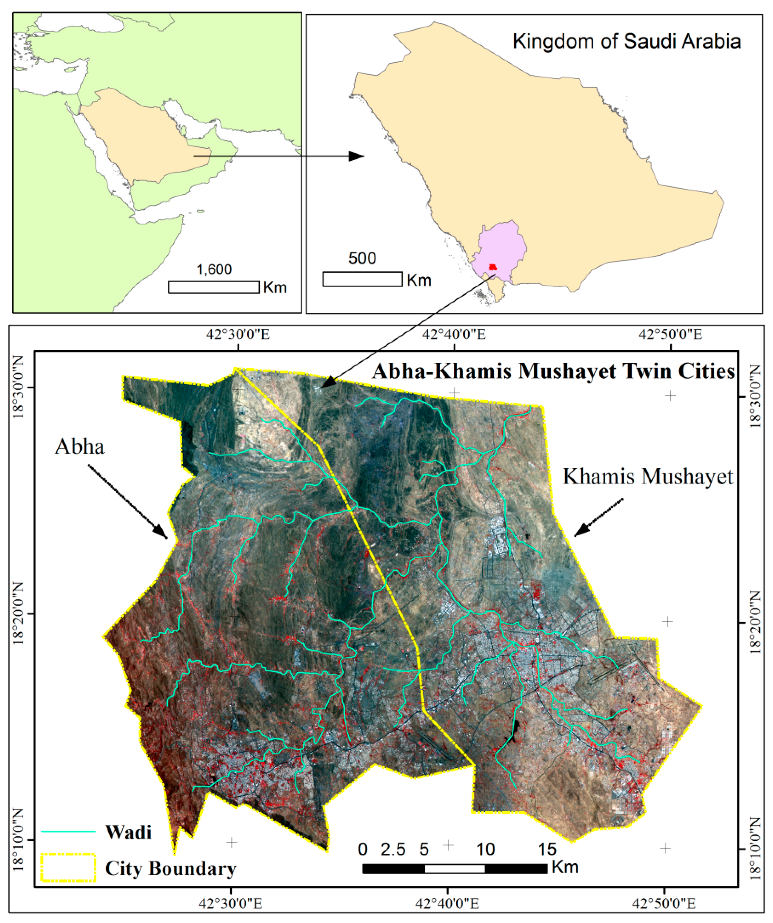
Figure 1. Study Area.
Atmosphere 11 00762 g001
Figure 2. Flow diagram for the adopted methodology.
Atmosphere 11 00762 g002
Figure 3. Graphical distribution of mean Land surface temperature (LST) and normalized difference vegetation index (NDVI) in different land use/land cover (LULC) class.
Atmosphere 11 00762 g003
Figure 4. Spatial distribution of LST (a), LULC (b), NDVI (c), DEM (d), Aspect (e), and Slope (f).
Atmosphere 11 00762 g004
Figure 5. Histogram profile of NDVI and LST over different LULC.
Atmosphere 11 00762 g005
Figure 6. Linear regression coefficient between LST and NDVI for LULC class as a whole, dense vegetation, agricultural land, and sparse vegetation.
Atmosphere 11 00762 g006
Figure 7. A profile map drawn along the Abha wadi (a); linear regression between LST–NDVI along the Abha wadi (b); linear regression between LST–elevation along the Abha wadi (c) and graphic representation of the data distribution of NDVI and LST along the Abha wadi; elevation variability and closer field of view of the False Color Composite Image of ASTER to their respective boxes (i.e., red) (d).
Atmosphere 11 00762 g007
Table 1. Comparison of field observation temperature with satellite LST observation.
FeaturesGround Based Measurements on 24–27 June 2019 (10.00–11.30 Local time) in °CSatellite Observation
ASTER 26 June 2019 °C
GCS Coordinates WGS 84 Decimal Degrees
Dense Vegetation29.46 °C31.26 °C42.587765 E 18.251733 N
Concrete (built-up)41.12 °C43.29 °C42.724764 E 18.302471 N
Asphalt (Parking)50.42 °C48.77 °C42.560936 E 18.252881 N
Exposed Rocky area52.45 °C50.52 °C42.617576 E 18.389468 N
Table 2. The LST and NDVI and their SDs in various LULC class, calculated through zonal statistics analysis using ArcGIS.
LULC Class NameNDVILST in °C
MinMaxMeanSDMinMaxMeanStd.dev.
Built up−0.020.120.06050.02125.4052.6944.443.339
Waterbodies0.020.110.04410.02222.0037.1725.752.568
Dense Vegetation0.150.500.2420.05426.1743.5036.882.783
Sparse Vegetation0.100.300.16330.04430.3549.2140.623.255
Agricultural0.100.380.17120.05431.2949.3340.853.202
Scrubland0.010.160.08480.021724.6854.3143.533.061
Baresoil0.010.090.06030.011133.5951.5443.772.569
Exposed Rock−0.020.080.05580.013228.6055.1745.673.238
Table 3. Statistical analysis LST and NDVI over the various LULC at the classified elevation zone.
LULC1564–20002001–21002101–23002301–25002501–2736
AreaMean NDVIMean LSTAreaMean NDVIMean LSTAreaMean NDVIMean LSTAreaMean NDVIMean LSTAreaMean NDVIMean LST
Built-up43.340.06146.14166.220.06744.4462.820.08242.4612.440.10441.331.180.12339.29
Waterbodies------0.390.07228.550.1620.07628.020.020.17627.01------
Dense Vegetation0.920.16641.151.390.15238.373.390.16238.101.940.15737.710.490.17633.95
Sparse Vegetation2.920.13043.8110.910.11942.5915.700.13340.9622.380.13639.7318.830.14638.46
Agricultural Cropland3.370.13242.965.400.11742.912.020.14141.030.650.12940.570.420.14239.23
Scrubland66.590.07245.40162.190.08043.7273.770.09342.8724.850.11041.128.690.12840.02
Baresoil43.790.05944.9356.950.06742.914.550.07242.520.020.06641.470.110.11638.76
Exposed Rocks85.480.05547.71165.100.06145.70183.380.06843.7418.190.09240.910.020.10235.25
Table 4. Statistical analysis LST and NDVI over the aspect classes at the classified elevation zone.
Aspect1564–20002001–21002101–23002301–25002501–2736
AreaMean NDVIMean LSTAreaMean NDVIMean LSTAreaMean NDVIMean LSTAreaMean NDVIMean LSTAreaMean NDVIMean LST
Flat30.07246.346.40.07743.931.60.10042.840.180.11040.060.090.16138.74
North (0–22.5 and 337.5–360)290.06546.2271.60.07444.3539.20.08642.8280.12039.922.670.14438.15
Northeast (22.5–67.5)410.06246.5892.50.07144.725810.08243.7314.70.11241.156.250.13739.57
East (67.5–112.5)340.06247.0583.60.06844.8965.60.07744.0719.10.10742.266.820.13540.81
Southeast (112.5–157.5)260.06147.1160.10.06644.8243.40.07243.809.50.10841.253.00.13239.69
South (157.5–202.5)230.06546.4056.40.06644.4331.90.07942.785.80.11039.862.340.13538.30
Southwest (202.5–247.5)310.06445.2362.80.06943.8633.90.07942.098.30.12038.643.530.13835.93
West (247.5–292.5)320.06545.0368.80.07343.6938.60.08241.899.40.12038.513.080.14735.84
Northwest (292.5–337.5)270.06745.6668.90.07743.9035.60.08542.326.00.12638.972.160.15136.57
Table 5. Statistical analysis LST and NDVI over the slope classes at the classified elevation zone.
Slope in Degree1564–20002001–21002101–23002301–25002501–2736
AreaMean NDVIMean LSTAreaMean NDVIMean LSTAreaMean NDVIMean LSTAreaMean NDVIMean LSTAreaMean NDVIMean LST
0.00–3.00178.660.06646.45395.40.07344.43107.580.08643.136.860.12140.741.590.13639.56
3.01–7.0060.240.05945.97150.40.06744.37150.600.07843.4422.250.11540.856.470.14139.22
7.01–13.005.200.06443.8222.100.06743.8570.100.07543.0130.340.11240.6511.280.14038.88
13.01–23.000.790.05739.081.800.06642.7915.720.07441.6619.540.11140.469.230.14138.70
23.01–59.862.120.03236.671.520.06636.213.750.08736.781.990.12039.701.390.15037.48
Table 6. Research findings relationships between LST and NDVI.
DataStudy AreaAuthorsResults
Landsat−7 Delhi, India[58]LST-NDVI showed a negative correlation
ASTERDelhi, India[20]Day-Night LST with impervious surface, positive correlation
Landsat-5 & Landsat-7 South Karkheh, Iran[88]LST-NDVI showed a negative correlation
Landsat-5Shenyang, China[87]“LST and NDVI scatter plots showed triangle relation, the three directions represent water area, green land and cultivated land, construction land, respectively”
Landsat-5Guilin, China[89]LST-NDVI showed a negative correlation
Landsat-8Guizhou, China[90]“LST and NDVI scatter plots showed an obtuse-angled triangle distribution”
ASTERAbha, Saudi ArabiaCurrent research LST-NDVI showed a negative correlation and NDVI scatter plots showed an “obtuse-angled triangle” distribution