Article

Evaluation of Historical CMIP5 GCM Simulation Results Based on Detected Atmospheric Teleconnections

1
Department of Meteorology, Eötvös Loránd University, Pázmány P. s. 1/A, H-1117 Budapest, Hungary
2
Excellence Centre, Faculty of Science, Eötvös Loránd University, Brunszvik u. 2, H-2462 Martonvásár, Hungary
3
Faculty of Forestry and Wood Sciences, Czech University of Life Sciences Prague, Kamýcká 129, 165 21 Prague 6, Czech Republic
*
Author to whom correspondence should be addressed.
Atmosphere 2020, 11(7), 723; https://doi.org/10.3390/atmos11070723
Submission received: 27 May 2020 / Revised: 30 June 2020 / Accepted: 2 July 2020 / Published: 7 July 2020

Abstract

:
Atmospheric teleconnections are characteristic to the climate system and exert major impacts on the global and regional climate. Accurate representation of teleconnections by general circulation models (GCMs) is indispensable given their fundamental role in the large scale circulation patterns. In this study a statistical method is introduced to evaluate historical GCM outputs of the fifth phase of the Coupled Model Intercomparison Project (CMIP5) with respect to teleconnection patterns. The introduced method is based on the calculation of correlations between gridded time series of the 500 hPa geopotential height fields in the Northern Hemisphere. GCMs are quantified by a simple diversity index. Additionally, potential action centers of the teleconnection patterns are identified on which the local polynomial regression model is fitted. Diversity fields and regression curves obtained from the GCMs are compared against the NCEP/NCAR Reanalysis 1 and the ERA-20C reanalysis datasets. The introduced method is objective, reproducible, and reduces the number of arbitrary decisions during the analysis. We conclude that major teleconnection patterns are positioned in the GCMs and in the reanalysis datasets similarly, however, spatial differences in their intensities can be severe in some cases that could hamper the applicability of the GCM results for some regions. Based on the evaluation method, best-performing GCMs can be clearly distinguished. Evaluation of the GCMs based on the introduced method might help the modeling community to choose GCMs that are the most applicable for impact studies and for regional downscaling exercises.

1. Introduction

Atmospheric teleconnections are persistent, large-scale phenomena that link the variability of meteorological parameters across large geographical distances. Teleconnections are studied by the identification of distant geographical areas with co-varying meteorological state variables and are visualized by teleconnection patterns. The most intense regions of the teleconnections are called action centers [1,2,3]. Patterns of the large-scale atmospheric circulation in the Northern Hemisphere (hereinafter referred to as NH) were identified by Wallace and Gutzler [1] by examining teleconnectivity maps. These maps were obtained from the calculation of empirical correlations of gridded geopotential height datasets at the isobaric surface of the 500 hPa field (Z500). Horel [2] applied rotated principal component analysis (RPCA) on the Z500 to detect teleconnections. Barnston and Livezey [3] also conducted RPCA but on the geopotential height field at the 700 hPa isobaric surface for the detection of the teleconnections.
General circulation models (GCMs) are widely used to quantify climate change signal for historical time periods and for the future as well [4,5]. Reanalysis datasets provide observation-based, long term, high quality reference dataset for the climate system [6,7] that enables the comparison of GCM simulations with the real world circulation patterns. The number of studies dealing with the comparison of GCM outputs to reanalysis datasets has growing since the Coupled Model Intercomparison Project (CMIP) was launched within the framework of the World Climate Research Program (WCRP) in 1995. To get reliable results from GCM projections, identification of their associated large-scale circulation systems is required to benchmark their ability to simulate the major circulation features including the location of the polar front, the jet stream, and the synoptic systems. As teleconnection patterns are supposed to be represented by state-of-the-art GCMs, their analysis provides a mechanism to evaluate the quality of GCMs [8].
In the last decade, numerous studies focused on the datasets of the fifth phase of the CMIP (CMIP5), which were disseminated within the framework of the Fifth Assessment Report (AR5) of the Intergovernmental Panel on Climate Change (IPCC) [5]. A growing number of studies focus on winter circulation patterns in the NH in the Euro-Atlantic region [9,10,11,12]. Teleconnections and their effects on atmospheric variables were also studied in the region of the Mediterranean Sea both by using regional climate models (RCMs) [13,14] and GCMs [15]. Recently, the connection between teleconnections detected in the Eurasian region (e.g., the East Atlantic/West Russia and the Scandinavian patterns) and distant areas in Asia were examined [16] while in the region of the Pacific Ocean, among others, the North Pacific Oscillation (NPO) was analyzed [17].
To assess the possible socio-economic effects of the changing climate in the 21st century is a highly relevant task. For that purpose, GCM results are used in downscaling exercises to provide regional scale, relatively fine resolution projections, i.e., RCM outputs, for impact studies [8,18,19,20]. Since RCMs are driven by GCM outputs [21,22], GCM biases may affect the results obtained from RCMs [23]. Consequently, incorrect representation of the teleconnections directly affects RCM results and has the potential to provide a false climate change signal. Exploitation of GCMs that are characterized by biased circulation patterns could seriously jeopardize policy relevant decisions.
Various studies attempted to rank GCMs of the CMIP5 by using different model metrics [11,12,24,25,26,27]. In this study we introduce a method with the aim to rank the GCMs with respect to the location and intensity of the teleconnections. For that purpose, first an information entropy-computing technique (a simple diversity index-calculation method) is applied on the correlation fields of the Z500. Those diversity fields are adequate to decide whether or not a teleconnection pattern is stable in time in a specific region. Second, the position of pairs of grid cells with a strongly co-varying geopotential height time series (i.e., potential action centers) is examined by fitting a local polynomial regression model on them. GCM evaluation is done by quantitative comparison of diversity fields and regression models to those obtained from the reanalysis datasets. Results of the comparisons are used to select the best-performing GCMs taking into account both quality metrics.
The study contributes to the practical applicability of GCM outputs in regional downscaling exercises and impact studies. Though the study focuses on the CMIP5 dataset, the introduced method can be applied on any other GCM.

2. Data and Methods

2.1. Data

Signals of atmospheric teleconnections are detected in the Z500, as it was demonstrated that teleconnections, e.g., the signals of the North Atlantic Oscillation (NAO), become stronger with increasing altitude in the troposphere [28].
Two atmospheric reanalysis datasets were used in the study to provide observation based reference for the geographical location and magnitude of the teleconnections. Those are the twentieth century reanalysis (hereinafter referred to as ERA-20C) of the European Centre for Medium-Range Weather Forecasts (ECMWF; [6]), which is available for the period of 1900–2010, and the NCEP/NCAR Reanalysis 1 (hereinafter referred to as NCEP-NCAR R1; [7]) of the National Centers for Environmental Prediction (NCEP) and the National Center for Atmospheric Research (NCAR), which provides data from 1948 to present. The spatiotemporal resolution and time coverage of these two reanalysis datasets are adequate to validate historical GCM outputs. The usage of multiple reanalysis products is beneficial because of their differences in the ability to reproduce low-frequency atmospheric circulation in the troposphere [29]. Due to the expected differences between the two reanalysis datasets, different ranking of GCMs is expected [30].
The climate signal of teleconnections can be detected on decadal or longer time scales, consequently 10-year-long and 30-year-long periods were examined. The analysis of 30-year-long periods is beneficial because the average position of the teleconnections can be determined while the selection of 10-year-long periods provides us with enough data to conduct analysis on the potential action centers. The identification method was applied on the daily temporal resolution because action centers, e.g., in case of the less-intense teleconnection in the region of the Mediterranean Sea, can fade away if weekly or monthly time aggregation is used. In this study six 30-year-long and ten 10-year-long overlapping periods were investigated for the period of 1951–2005. The 30-year-long periods were 1951–1980, 1956–1985, 1961–1990, 1966–1995, 1971–2000, and 1976–2005 while the 10-year-long periods were 1951–1960, 1956–1965, 1961–1970, 1966–1975, 1971–1980, 1976–1985, 1981–1990, 1986–1995, 1991–2000, and 1996–2005.
This period selection logic was supported by the temporal availability of the historical Z500 GCM datasets, which are available on a daily scale mainly for the interval from 1951 to 2005 [31]. Only winter months (December, January, and February) were examined in this study when the effects of large-scale atmospheric circulation are the most prominent. To get an equally long time series, only 30 days were kept in December and January while 28 days were kept in February. To reduce seasonality and noise in the data obtained from the Z500 fields, detrended and standardized daily anomaly datasets were created. For that purpose, first, daily means from the averaging period were subtracted from each daily data to calculate anomalies. Then, the anomalies were divided by the daily standard deviations for the averaging period. Finally the linear trend was removed by fitting least square regression [32].
GCM datasets were selected from the CMIP5 project [31] and data were accessed via the website of the German Climate Computing Centre (DKRZ) (https://esgf-data.dkrz.de/projects/esgf-dkrz/). GCMs with atmospheric models that are characterized by at least 2.5° × 2.5° original horizontal resolution were analyzed. After careful consideration and analysis of the CMIP5 database, 19 GCMs were selected that fulfilled the requirements. The full list of GCMs that are used in this study are listed in Table 1. The simulation outputs were interpolated to the common 2.5° × 2.5° horizontal grid by applying bilinear interpolation, which means 37 × 144 grid cells in the NH. This model selection and interpolation method was used to minimize the inevitable errors introduced by interpolation.

2.2. Statistical Analysis

2.2.1. Identification of the Teleconnections

Teleconnections are defined as geographical areas with associated geopotential height time series that are negatively correlated with each other [1,3]. Identification of teleconnections is performed by the analysis of correlations between the time series of the Z500 field using the teleconnection method [1,48].
We applied our analysis on the basis of empirical Pearson correlation coefficients (hereinafter referred to as correlations), which are computed as follows. First, each of the Z500 time series was correlated with all the other Z500 time series. As a result, 37 × 144 correlation values were obtained concerning each grid cell from which the minimum value was selected and was referred as the strongest negative correlation [1,48]. Those were concentrated in several centers (i.e., local minima) as it is demonstrated in Figure 1 with blue-shaded dots. Then, pairs of grid cells were selected with identical strongest negative correlations indicating a one-to-one correspondence (i.e., mutually unambiguous correspondence between the selected grid cells). Each pair of grid cells connected two local minima. If the associated correlation value was statistically significant the pair can be the potential action center (hereinafter abbreviated as PotAC) of a single teleconnection. PotACs are also exemplified in Figure 1 with red circles, which are connected with red lines. In our analysis teleconnections were represented with PotACs, therefore teleconnections were considered as dipoles. Consequently, each grid cell of the PotAC represents a single pole of the teleconnection hereinafter referred to as pole.
To decide whether correlations were statistically significant or not, a permutation test was carried out. According to this method, time series of the Z500 field associated with each grid point in a PotAC were replaced with randomly generated data series. Subsequently, correlations with all the other time series were computed again. The limit of statistically significant correlations was determined by examining the distribution of the randomly generated correlations. This test was repeated 1000 times in the case of each pole. Two sets of random data series were constructed. In the case of the first set, we assumed that the original Z500 time series were the realizations of normally distributed random variables, therefore datasets were generated, which follow normal distribution. The parameters of the distribution were estimated by using the method of moments. In the case of the second set, the significance test was conducted on datasets, which were the random permutation of the original time series. The results suggest that strongest negative correlations below −0.3 could be considered to be statistically significant at a significance level of 0.1%.
Note that our analysis focused only on the NH because majority of the grid cells with statistically significant strongest negative correlations can be found here. This phenomenon is clearly visible in Figure 1. For the sake of brevity, the term strongest negative correlation hereinafter implies statistically significant correlations. Global correlation maps including PotACs for 30-year-long periods were exemplified by the NCEP-NCAR R1 in Figure S1 while correlation maps concerning only the NH for both reanalyses are shown in Figure S2 of the Supplementary Material. The similarity of Figure 1 and Figure S2b suggest that the applied method was less dependent on the selected area.
An investigation was carried out in the case of each reanalysis and GCM for all periods listed above in Section 2.1. It means the analysis of 21 × 6 cases for the 30-year-long periods and the examination of 21 × 10 cases for the 10-year-long periods.

2.2.2. Evaluation of the GCMs

In this study we evaluated the GCM performance by comparing historical model outputs with the results obtained from the two reanalysis datasets. Evaluation of the GCMs consists of the following two steps: (1) the comparison of the distribution of the strongest negative correlations using the temporal stability method, and (2) the analysis of spatiotemporal distribution of the PotACs.

GCM Evaluation: Stability Patterns

The first step of the GCM evaluation is the comparison of the distribution of the strongest negative correlations obtained from each GCM with those obtained from the reanalyses. An information entropy based method was applied, therefore a simple diversity index was constructed to quantify uncertainty. Details about the measurement of information entropy can be found in Shannon [49], Simpson [50], and Rényi [51]. In the case of each reanalysis and GCM with respect to each grid cell, the number of periods was determined when the strongest negative correlations were statistically significant. We restricted the analysis to the examination of strongest negative correlations below the 25th percentile of their distribution, which means that values below the 25th percentile were summarized in the case of 30-year-long and 10-year-long periods, respectively. This procedure enabled us to distinguish regions in the NH where the presence of teleconnections was considered to be stable in time. Furthermore, it facilitated the identification of grid cells containing substantial amount of information within the analyzed field. From this point of view, grid cells were the most common in which correlations below the 25th percentile never appeared while the most important grid cells were those where correlations below 25th percentile appear six (ten) times in the case of the six 30-year-long (ten 10-year-long) periods. The above defined diversity index was visualized in the form of maps and were referred to as stability patterns.
We assumed that GCMs did not perform equally well in every region relative to the reanalysis datasets. In order to take into account these GCM related differences and to avoid the arbitrary selection of the study region, Monte Carlo simulations were carried out based on the stability patterns. At first, the same 1% of the grid cells were selected randomly from each GCM and reanalysis dataset. Then, root-mean-square error values (RMSE) were computed between the selected GCM and the reanalyses to quantify their similarities/dissimilarities. To get significant results, this method was repeated 500,000 times. As a result, 500,000 × 19 RMSE values were calculated to evaluate each GCM with respect to each reanalysis dataset, both in the cases of 30-year-long and 10-year-long periods. Consequences are drawn from the distribution of those RMSE values. If the performance of a GCM (quantified by the RMSE) depends on the selection of the study region, the range between the minimum and maximum of its RMSE values will be larger.

GCM Evaluation: Loess

The second step of the GCM evaluation is the analysis of the distribution of the PotACs with the application of the local polynomial regression technique (locally estimated scatterplot smoothing, abbreviated as loess; [52]). Some GCMs might reproduce the spatial dimensions of the teleconnections accurately while some might fail to locate the PotACs accurately in comparison with the reanalyses. Since PotAC, which are pairs of grid cells, are typically aligned north-to-south in the reanalyses, the southerly and northerly located poles could be considered as parts of two hypothetical belts that surround the NH. Though the poles were not considered to be the realizations of continuous random variables, due to their large number in the case of the 10-year-long periods, regression curves fitted on them could be compared to each other. In this approach these regression curves were used to evaluate GCMs.
To fit regression curves, PotACs were used from all 10-year-long periods where the predictand (predictor) was the realization of geographic latitudes (longitudes). In accordance with Tukey’s method [53] based on the interquartile range (IQR), data were considered as outliers and were omitted when they fall outside the range defined by the IQR of the latitudes ±1.5∙IQR. After that, the values of the predictand, which belong to the same longitude were averaged. The span parameter was estimated by using the bias-corrected version of the Akaike information criterion [54].
Regression curves fitted on the PotACs obtained from the historical outputs of the GCMs were compared to the regression curves obtained from the reanalyses by calculating RMSE over a common area. To cover the largest possible area in the NH, regression curves were fitted on a map with an Atlantic view (from 177.5° W eastward to 175° E) and on another map with a Pacific view (from 0° eastward to 2.5°W). With this method a total of four regression models were fitted for each GCM and reanalysis dataset: two on the southerly located PotAC poles and two on the northerly located PotAC poles.
Based on the objective metrics described above, GCMs were ranked in terms of performance relative to the reanalysis datasets. Climate Data Operators [55] were used to pre-process data including to apply bilinear interpolation on the gridded datasets. Computation and visualization were carried out in the R statistical computing software version 3.6.1 [56]. Functions of the ncdf4 R package [57] were applied to handle netCDF files while the following R packages were used to plot the data (polar stereographic maps are created by the functions matrix.poly and val2col downloaded from the websites: http://menugget.blogspot.com/2012/04/create-polygons-from-matrix.html and http://menugget.blogspot.com/2011/09/converting-values-to-color-levels.html. Last accessed on 04.07.2020.): fields [58], maps [59], maptools [60], mapproj [61], and RColorBrewer [62]. The loess method was applied by the functions of the fANCOVA package [63].

3. Results

3.1. Teleconnections in the Reanalyses and the GCMs

According to the reanalyses, teleconnections can be identified in the NH in each examined time period over the North Pacific Ocean, over the North Atlantic Ocean, and in the region of the West Siberian Plain and the Gobi Desert (referred to as Asia). Teleconnections can be detected in almost all periods in the region of the Mediterranean Sea and the Red Sea (referred to as the Mediterranean region; Figure 1 and Figures S1 and S2 in the Supplementary Material). The most intense correlations were associated with grid cells over the North Pacific Ocean while the weakest correlations were detected in the Mediterranean region. This leads to less-pronounced local minima in the Mediterranean region if time-averaged strongest negative correlation fields were plotted (Figure S3 of the Supplementary Material). The two reanalysis datasets provided teleconnections with similar magnitudes, which was the consequence of the similarly distributed correlations exemplified by histograms in Figure S4 of the Supplementary Material. However some differences in the positions of the teleconnections could be observed especially in the Euro-Atlantic region (Supplementary Material Figure S2).
In the case of the GCMs, the strongest negative correlations (i.e., local minima) could be detected in similar areas as in the reanalyses (Supplementary Material Figure S3; all PotACs obtained from the GCMs are shown in Figure S5 in the Supplementary Material). However the magnitudes of those correlations were different in the case of some GCMs. With the exception of the HadGEM2-AO, the strongest negative correlation fields of the GCMs and the reanalyses were associated with median values between −0.3 and −0.35 regarding the 30-year-long periods while those were between −0.3 and −0.4 concerning the 10-year-long periods. The main difference was observable in the shape of the distribution of the strongest negative correlations. According to Supplementary Material Figure S4, the strongest negative correlations had left-skewed distributions in the reanalyses, which was less pronounced in some GCMs. As a consequence, GCMs underestimate the intensity of teleconnections relative to the reanalyses. The HadGEM2-AO was exceptional because it produced remarkably stronger correlations. The associated medians were below −0.4 for the 30-year-long periods and −0.6 for the 10-year-long periods.

3.2. Stability Patterns

3.2.1. Comparison of the Distribution of Stability Patterns

Figure 2 shows the spatial distribution of the number of 30-year-long (10-year-long) periods in which the strongest negative correlation was below the 25th percentile of the correlations in a given grid cell for selected GCMs and for the two reanalyses (note that the application of the 25th percentile means variable threshold for the reanalyses and also for the GCMs; see Section 2.2.2). Selected GCMs that are presented in Figure 2 were representative to the whole set of GCMs. (similar maps for all GCMs are shown in Figure S6 of the Supplementary Material) Stability of the teleconnection was increasing with an increasing number of time periods. A small, non-zero number in a specific grid cell indicates temporal changes in the intensity of the teleconnection in that cell, while zero means that teleconnection did not occur in any period (according to the method used in this study).
According to the stability patterns of the reanalyses presented in Figure 2, the most stable teleconnection was located in the region of the North Pacific Ocean. The second most stable could be detected in the North Atlantic Ocean. However, due to the eastward shift of the most intense regions of the teleconnection (Figures S1 and S2 in the Supplementary Material), the phenomenon shows more stability in the north-eastern part of the Atlantic Ocean. A stable but smaller teleconnection can be found in Asia. The least stable teleconnection was located in the Mediterranean region with correlations often not reaching −0.4 in this area.
Difference maps were created based on the stability maps to get further insight into the similarity/dissimilarity of the GCMs and the reanalyses, and also of the two reanalyses. Difference maps for selected GCMs are presented in Figure 3 while all maps can be found in Figure S7 of the Supplementary Material. In the followings we presented cases where differences between the two datasets were remarkably large. Concerning the 30-year-long periods (Figure 3a), over the south-eastern part of the North Pacific Ocean the teleconnection was more stable in the NCEP-NCAR R1 relative to the ERA-20C dataset. On the contrary, in the ERA-20C, teleconnections were more stable over a larger area in Asia and in the Mediterranean region compared to the NCEP-NCAR R1. In the case of the 10-year-long periods (Figure 3b) similar differences could be detected over the North Pacific Ocean as in case of the 30-year-long periods. However, over the eastern part of the North Atlantic Ocean, in the ERA-20C the number of periods with the strongest negative correlation below the 25th percentile was larger in comparison with the NCEP-NCAR R1 while the opposite was true for the western part of that region. This indicates a more easterly located teleconnection in the ERA-20C relative to the NCEP-NCAR R1.
In case of the GCMs similar consequences could be drawn from the examination of the 30-year-long and the 10-year-long periods. The GCMs typically reproduced the teleconnections in similar geographical areas as the reanalyses, but there were significant differences concerning their intensities and the position of the most intense regions (Figure 3). The GCMs captured the most stable regions of the teleconnection over the North Pacific Ocean relatively well, though there was a tendency to locate it north-eastward relative to the reanalyses. Major discrepancies were noticed over the North Atlantic Ocean. Several GCMs, e.g., the ACCESS1-0 and the HadGEM2-CC, reproduced the most stable part of the teleconnection over the western part of the North Atlantic Ocean while in some GCMs, e.g., the MPI-ESM-LR, the MPI-ESM-MR and the MPI-ESM-P, the teleconnection is captured with smaller intensity as in the reanalyses. In Asia more than half of the GCMs underestimate the stability of the teleconnection. The representation of the teleconnection in the Mediterranean region is considered to be poor. The GCMs tended to produce weaker correlations than the reanalyses with the exception of the MIROC5, the NorESM1-M, and the HadGEM2-AO. The main areas with the discrepancies in the cases of the MIROC5 and the NorESM1-M were the North Pacific region and the subtropical areas. As it was mentioned, correlation field associated with the HadGEM2-AO was remarkably intense compared to any other reanalyses/GCMs (Supplementary Material Figure S3). However, red-shaded areas in Figure 3 imply an underestimation of teleconnections relative to the reanalyses. The reason behind this finding is the following. The HadGEM2-AO did not capture the structure of teleconnections, which were detected in the reanalyses and in other GCMs, but teleconnections covered almost the entire NH. As a consequence, the correlations were not as intense in those regions where teleconnections were detected in the reanalyses.

3.2.2. Comparison of Stability Patterns Based on Monte Carlo Simulations

In order to quantitatively analyze the performance of the models, the stability pattern of each GCM was compared with the stability patterns of the two reanalyses. As a reference the two reanalyses were also compared to each other (quantiles of the calculated RMSE values can be found in Table S1 of the Supplementary Material). We distinguished four cases depending on the chosen reanalysis and the length of the time periods analyzed. Results of the Monte Carlo simulations are summarized in the form of boxplots in Figure 4.
If the median values of the RMSE values—henceforth referred to as the RMSE median—are examined then the largest similarities are observable between the two reanalyses with an RMSE median of 1 (Figure 4; red dots). The RMSE median obtained from all GCMs was 2 and 2.5 based on the examination of 30-year-long and 10-year-long periods, respectively (red lines in Figure 4). Consequently, the analyzed GCMs differed from the reanalyses with 2–2.5 time periods on average, which was higher than the RMSE median associated with the reanalyses. In all four cases, the RMSE median of the ACCESS1-0, the CMCC-CM, the CMCC-CMS, the GFDL-ESM2M, the HadGEM2-CC, the MPI-ESM-LR, and the MPI-ESM-P were below the RMSE median obtained from all GCMs.
For each reanalysis/GCM pairs the difference between the RMSE median obtained from the Monte Carlo simulations and the RMSE value calculated for the entire NH was negligibly small (<0.05). Consequently, the median values could not be used to quantify area-sensitivity of the GCMs. For that purpose, the range between the maximum and minimum values of the distributions of the RMSE values—hereinafter referred to as the RMSE range—were applied. RMSE ranges associated with the reanalyses were remarkably smaller than those associated with the GCMs. There was no simulation among the half-million in which the RMSE exceeded two while the RMSE range for the GCMs was three on average in all four cases presented in Figure 4. With a few exceptions, the RMSE ranges increased with increasing RMSE median. Note that a relatively small range did not necessarily imply good overall GCM performance in all areas, which can be exemplified by the HadGEM2-AO (Figure 4). In the worst cases the RMSE range exceeded 3.5 while the largest RMSE values even reached or exceeded the RMSE value of 4 (e.g., in the case of the MRI-ESM1; Figure 4).
The variability of the RMSE values (therefore the RMSE range) was larger when 10-year-long periods were examined. Therefore, we avoided the comparison of RMSE values against each other obtained from the analysis of time periods with different lengths. To get further information regarding the sensitivity of the GCMs with respect to the selected area/reanalysis, the GCMs were plotted on the two-dimensional space defined by the RMSE medians and the RMSE ranges. The results are presented in Figure 5 for the four cases presented in Figure 4. In general, the distribution of the GCMs shows a large similarity in all four cases. However, some discrepancies can be noticed. The CMCC-CMS performs exceptionally well in all four cases with relatively small RMSE medians and RMSE ranges. Two other GCMs performed similarly well as the CMCC-CMS, namely the MPI-ESM-LR on shorter time scales and the HadGEM2-CC when the ERA-20C was used as a reference dataset. Largest discrepancies relative to the reanalyses were associated with the HadGEM2-AO and the MRI-ESM1, which were considered as offscale GCMs in Figure 5.

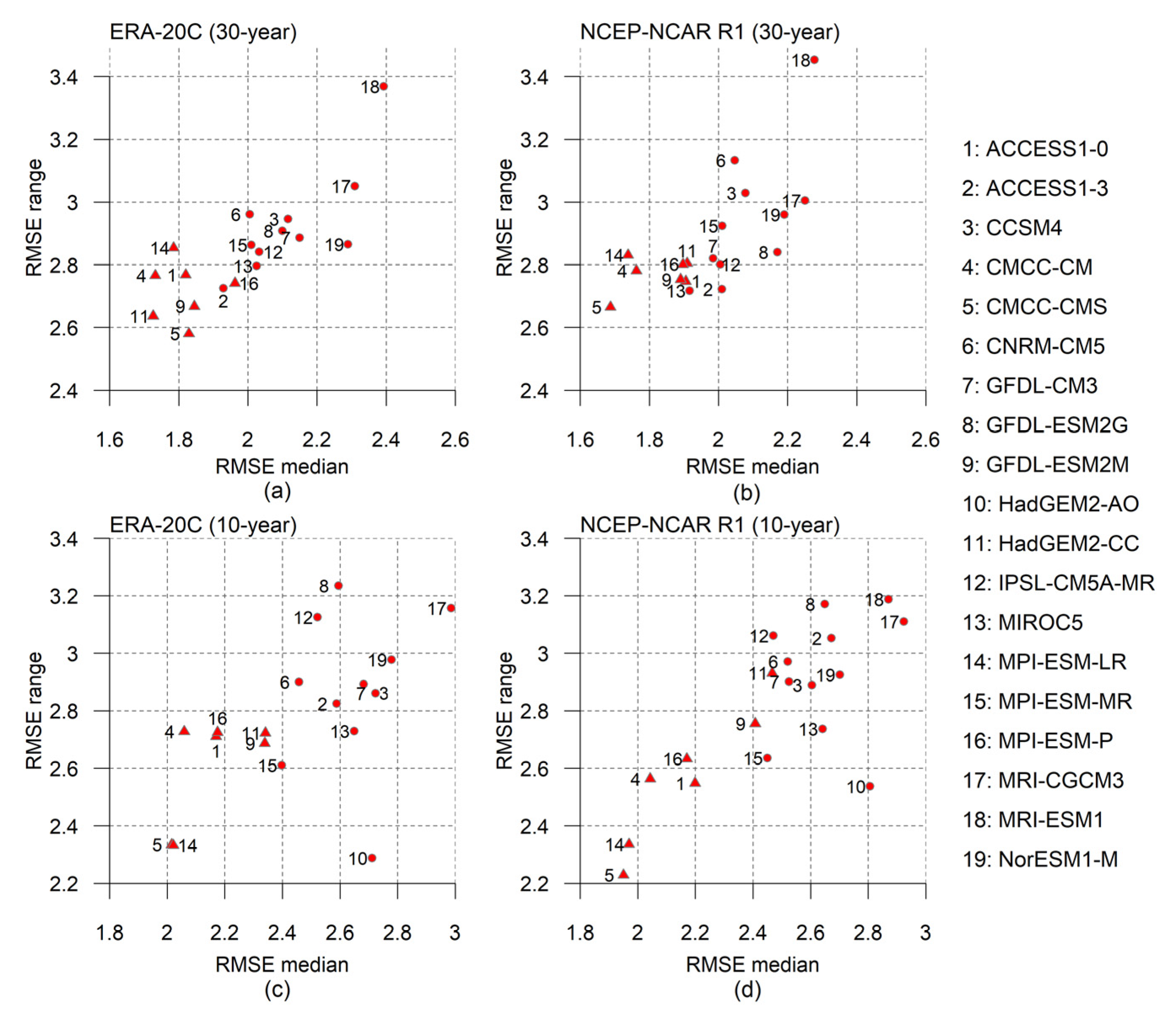
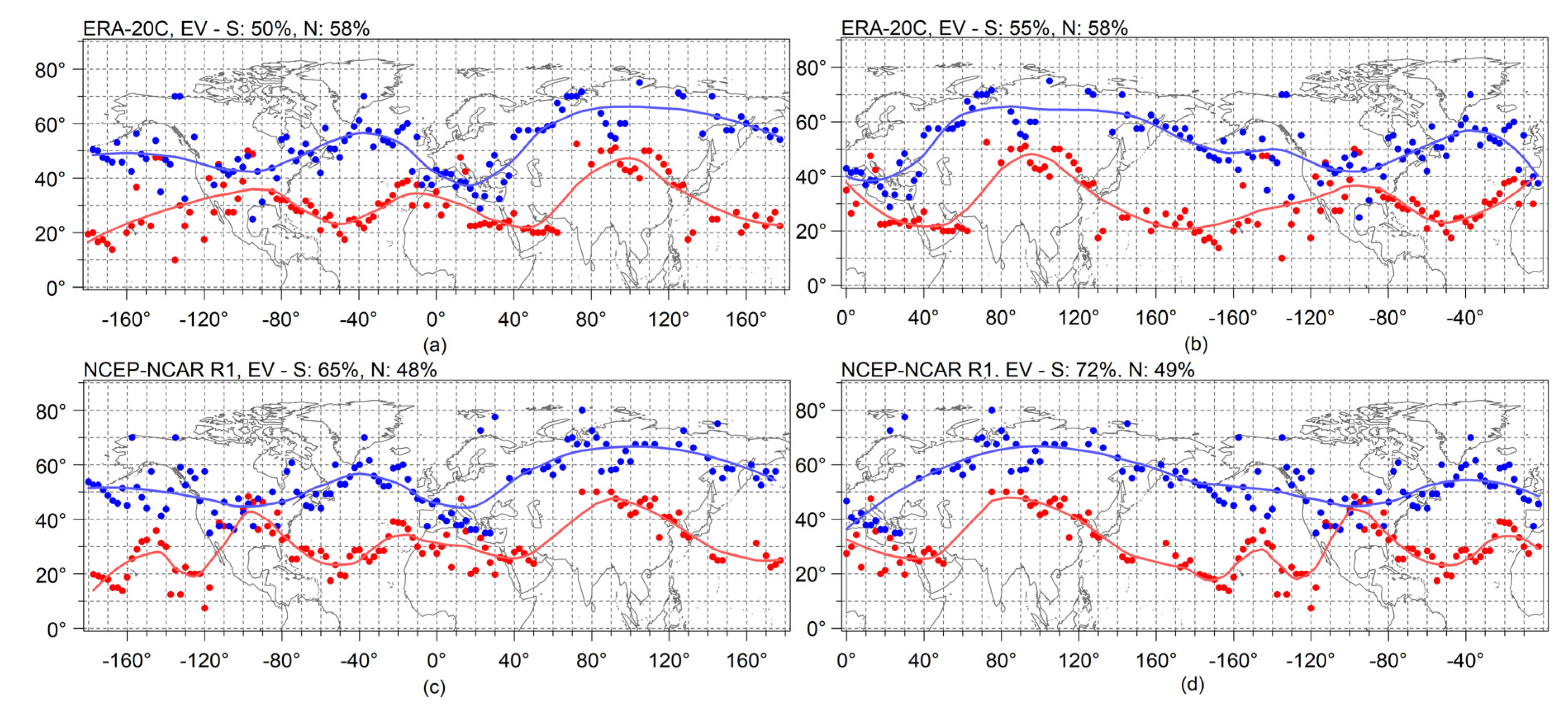
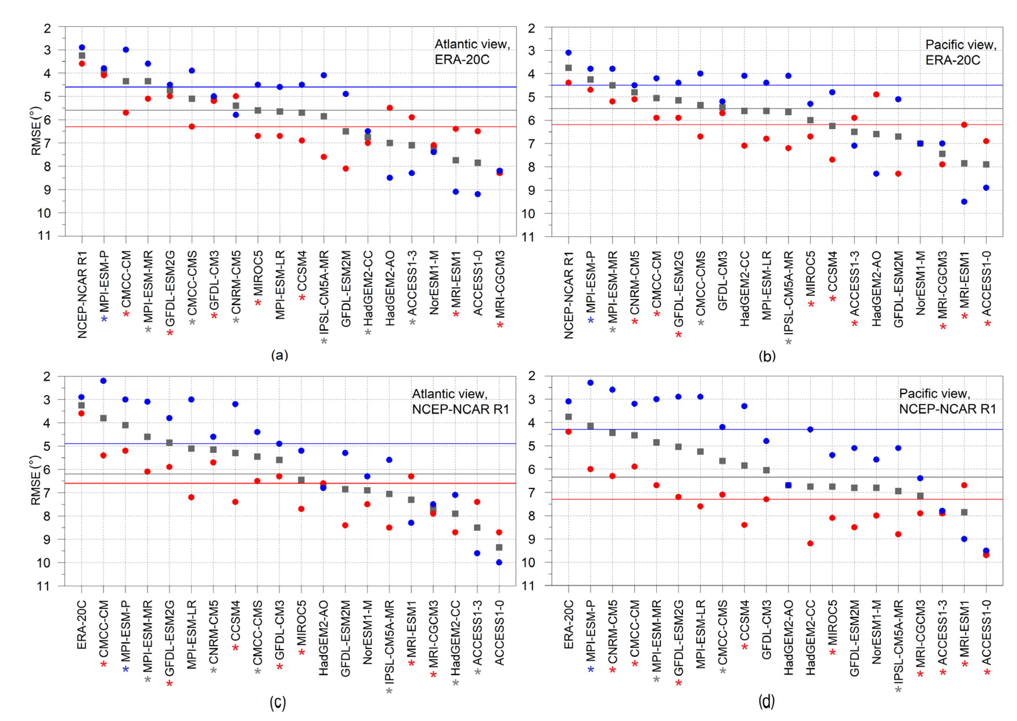
3.3. Comparison of Loess-Based Regression Applied on the PotACs

Loess regression curves fitted on the PotACs in the case of the reanalyses are shown in Figure 6 while regression curves of selected GCMs and their comparison against the reanalyses can be found in Figure 7. Maps for all GCMs are presented in Figure S8 of the Supplementary Material. Parameters of the loess models (span parameter, explained variance (EV), and residual sum of squares (RSS)) are presented in Table S2 of the Supplementary Material. We would like to stress here that the PotACs were not supposed to be present in the fitted curve in all locations (i.e., their geographical areas were localized rather than continuous in space). We used the fitting technique to quantify the similarity/dissimilarity between the observation based and the modeled circulation patterns.
In the case of the reanalyses the PotAC poles surround the planet in two hypothetical belts (hereinafter referred to as southern and northern belts), which are more pronounced above oceanic areas compared to continental areas due to the larger number of PotACs over the oceans as it can be seen in Figure 6. Each of the loess regression curves represents one of those belts. In general, the distance between the southerly and the northerly located regression curves was smaller in continental regions than above the oceans. The reanalyses were rather similar with RMSE values between 2.9° and 4.4° (RMSE values are presented in Table S3 of the Supplementary Material). The agreement between the two reanalyses was larger in the Euro-Atlantic region than in the region of the North Pacific Ocean and over North America. The above-mentioned areas were regions where teleconnections were detected, consequently the application of maps with an Atlantic and Pacific view that are centered on those regions was highly beneficial. The RMSE value between the loess regression curves centered on the North Pacific Ocean reached 4.4° in the southern belt. Smaller but remarkable differences could be found in the Middle East region. Regarding the northern belt smaller discrepancies could be detected with RMSE values between 2.9° and 3.1°. The largest difference was found over Europe.
In the case of the GCMs, generally higher EVs can be computed for the loess models fitted in the southern belt than in the northern belt. Relatively low EV values were associated with the distribution of the PotAC poles, which were more scattered in some GCMs than in the reanalyses. A good example is the MPI-ESM-P with respect to the southern belt or the HadGEM2-AO for which the NH was mostly covered by PotACs (Figure S5 in the Supplementary Material). Due to this anomalous behavior those GCMs were unable to reproduce the shape of the loess regression curves obtained from the reanalyses.
RMSE values associated with each GCM and medians for all GCMs are presented in Figure 8. We chose the best-performing GCMs from those that had EVs at least around 50% for all four loess models (i.e., models fitted on the Atlantic and Pacific view in the southern and northern belts). The CMCC-CMS and the MPI-ESM-MR were those GCMs that met the above-mentioned criterion and were among the best-performing 50% of the GCMs in all cases based on their RMSE values. According to their associated RMSE values, the MPI-ESM-P and the CMCC-CM could also be considered as best-performing GCMs, though their associated EVs were around or below 30% at least in one case, therefore the quality of those loess models were considered as poor. It is worth mentioning that the CNRM-CM5 was unique among the examined GCMs because its RMSE values obtained from the two belts were relatively close to each other in most cases. This implies good performance in both belts.
Regarding the CMCC-CM and the MPI-ESM-MR similar RMSE values can be obtained from the loess models fitted on maps with Atlantic and Pacific views (the largest difference was smaller than 0.6). Concerning the southern belt, major discrepancies can be observed not only in the North Pacific region but also in the Euro-Atlantic region. Over North America their regression curves were neither similar to the ERA-20C nor to the NCEP-NCAR R1. The associated RMSE values regarding the CMCC-CMS were between 6.3° and 7.1° while RMSE values were between 5.1° and 6.7° in the case of the MPI-ESM-MR. With respect to the northern belts a high degree of similarity can be noticed in the North Atlantic region. The largest discrepancies were observable over the North Pacific region. It is worth mentioning that over Europe the loess regression curve obtained from the MPI-ESM-MR was closer to the regression curve of the NCEP-NCAR R1. RMSE values associated with the CMCC-CMS were between 3.9° and 4.4° while the RMSE values obtained from the MPI-ESM-MR were between 3° and 3.8°.
As the reanalyses show significant differences in the above-mentioned regions in the NH, the similarity between some GCMs and the given reanalysis was higher than the similarity between the two reanalyses, which was never observable during the analysis of the stability patterns in Section 3.2.

3.4. Synthesis

Based on the comparison of the results of the stability patterns and the loess regression curves, the CMCC-CMS was the only GCM that performed well with respect to both aspects (i.e., the stability patterns and loess regression curves) for both the 30-year and 10-year periods. The MPI-ESM-LR, the MPI-ESM-MR, and the MPI-ESM-P performed relatively well for the 10-year-long periods, however not for both aspects. The MPI-ESM-LR and the MPI-ESM-P performed better in the case of the analysis of the stability patterns while the MPI-ESM-MR was among the best-performing GCMs when loess regression curves were examined. The GFDL-ESM2M and the HadGEM2-CC were only among the best-performing GCMs when 30-year-long periods were analyzed, consequently those were not expected to perform well in the analysis of loess curves, which was only performed on 10-year-long periods. The MRI-CGCM3, the MRI-ESM1, and the NorESM1-M were among the least precise GCMs concerning both aspects. Results obtained from the HadGEM2-AO shall be treated with caution due to the anomalously low correlations produced by that model.

4. Discussion

In our study circulation patterns of GCMs were compared to those of two selected reanalyses, which means that reanalyses were considered as the appropriate realizations of the atmospheric processes. However, as it is suggested by Stryhal and Huth [30], the selection of the reanalysis as a reference dataset may have important effects on the GCM validation. Stryhal and Huth [30] pointed out on the basis of the statistical comparison of reanalyses of winter circulation patterns in different Euro-Atlantic sectors that the agreement between the ERA-20C and the NCEP-NCAR R1 was relatively good with the exception of the Icelandic and the Eastern Mediterranean region. Recently, studies claim that reanalyses have limited value as they represent only one realization of the many hypothetical atmospheric circulations. They propose to use an ensemble of climate model simulations to understand the behavior of the climate system, thus the teleconnection systems [64,65]. Since state-of-the-art reanalyses are considered to be the best possible reconstructions of the real atmospheric circulations, they are indispensable to quantify existing circulation patterns, with some degree of uncertainty. In our study the application of two different reanalyses enabled the quantification of uncertainties related to the detection of teleconnection systems.
The analysis of the correlation fields obtained from the Z500 is used as an objective tool for detecting teleconnections. Principal component analysis (PCA) is widely used in the literature to analyze atmospheric circulations and to evaluate GCMs. There are studies that apply PCA [9,10] while other studies use its rotational version (RPCA) [11,12]. There is no consensus about which version of PCA should be used [32,66]. Here we claimed that the correlation field analysis is a suitable alternative of the RPCA because of the simpler interpretation of the results that is more consistent with the observations. By computing correlations, PotACs are considered to be parts of teleconnections, and their uncertainty is quantified by associated significance levels. In PCA patterns, opposite-signed grid cells do not necessarily imply codependency [67], therefore the detection of teleconnection. Furthermore, the number of principal components (PCs) that are rotated should be carefully chosen to avoid both under and over-rotation. The former may lead to loss of information on relevant signals while the latter may lead to the over-regionalization of the signals [68].
The method of the teleconnection analysis affects the appropriate detection of the signal, thus the result of the GCM evaluation. The application of the teleconnection identification method proposed by Wallace and Gutzler [1] was used in this study. This technique enables the detection of teleconnections over the North Pacific Ocean and the North Atlantic Ocean as well as in regions of the Mediterranean Sea and the inner part of Asia simultaneously, which may indicate the presence of oscillations such as the NPO and the NAO. In our method the NH was not divided into different areas to detect atmospheric patterns such as the NAO or teleconnection in the region of the Mediterranean Sea. In the case of NAO, PCA can be performed over an Atlantic sector [5] but the boundaries of the target area are not precisely defined. Concerning the Mediterranean region, a predefined domain between 30° N–60° N and 30° W–40° E is recommended to be analyzed [69]. Clearly, subjective selection of the target domain affects the results of PCA [66]. The presented method does not suffer from subjective decisions on the domain selection, which is an advantage compared to the PCA method.
By the application of the teleconnection method, based on the time series associated with the PotACs, teleconnection indices can be constructed similarly to the mobile index introduced by Portis et al. [70]. With those teleconnection indices shifts in the position of the most intense regions of the teleconnections can be examined and their relationships with atmospheric variables in distant areas can be identified. Monitoring shifts in the circulation patterns due to anthropogenic forcing is an important task, i.e., expansion of the Hadley cell is studied in Lu et al. [71] using GCM outputs. The NAO moved easterly in the last few decades of the 20th century [72], though this tendency cannot be observed in the years after the millennium due to less intense westerly winds [73]. The eastward shift can also be observed over the North Pacific Ocean where the Aleutian low relocated eastward after 1970 [74]. Correlation maps obtained from the reanalyses and presented in Figure S1 of the Supplementary Material are in accordance with those detected eastward shifts over the oceanic areas. Furthermore, on correlation maps closer to the present (Figure 1) it is clearly visible that the above-mentioned eastward shift over the North Atlantic Ocean cannot be observed anymore. According to our comparisons, only a few GCMs (e.g., the CMCC-CMS) captured the eastward shift of the most intense regions of the NAO (Figure S5 of the Supplementary Material). In the region of the North Pacific Ocean the larger part of the GCMs relocated the most intense regions of the teleconnections more easterly than the reanalyses. Exceptions were, for example, the CMCC-CMS in the case of the 30-year-long time periods and MPI-ESM-MR in the case of the 10-year-long time periods.
Our analysis was based on the examination of Pearson correlation fields, therefore linear components of the teleconnections were analyzed. However, nonlinear components may also have an important role to govern atmospheric processes, thus atmospheric circulation and their shifts [75]. In the last decade studies applying nonlinear approach became popular, for example using the method of self-organizing maps [76]. In the present approach the linear method was used for simplicity, but it is possible to extend it to take into account both linear and nonlinear effects.
We applied an information theory-based statistical method on the correlation fields of different time periods to evaluate the quality of CMIP5 GCMs. Usage of the diversity index and the loess-method enabled the evaluation of GCMs with respect to the intensity of various teleconnections without fading their signals. The application of information entropy to evaluate atmospheric models and to examine atmospheric teleconnections is gaining popularity recently [77,78]. The usage of the loess-method as a GCM evaluation tool with respect to atmospheric teleconnections is a novel method to the authors’ knowledge. As it was demonstrated, comparing GCM regression curves against the reanalysis regression curves by calculating RMSE values are not sufficient to select the best-performing GCMs. The quality of the regression (i.e., EV) should also be taken into consideration.
The results of our analysis are in line with other studies. According to Stryhal and Huth [11] the HadGEM2-CC is also among those GCMs that simulate the winter atmospheric circulation well in the Euro-Atlantic region on a longer time scale (i.e., 1961–2000). In our analysis the HadGEM2-CC performed well on longer time scales. According to our findings that the CMCC-CMS could be chosen as the best-performing model might be connected to the fact that the CMCC-CMS is a GCM in which the atmosphere is vertically well resolved [79]. Atmospheric processes in the upper-troposphere and the lower-stratosphere can modulate teleconnections. Feldstein [28] pointed out that the signal of NAO intensifies with increasing height. A recent study [80] found that the CMCC-CMS is able to reproduce climate change in the North Pacific region in winter relative to a reanalysis dataset. However, it relocates the geopotential height anomalies over the North Pacific Ocean southerly.
To evaluate the circulation pattern of GCMs, computing model metrics (e.g., RMSE) using the fields of significant correlations and establishing a GCM-ranking for each period and arbitrary-selected areas in the NH would provide little practical information because of the followings. (1) The GCMs must perform equally well both within the regions where teleconnections are detected and outside of them as well. If we restrict the analysis to some predefined areas where teleconnections can be detected, then GCMs (e.g., the HadGEM2-AO and the NorESM1) that perform less reliably outside those regions might be (incorrectly) considered to be of similar quality than GCMs that perform well in extensive areas (e.g., the CMCC-CMS and the HadGEM2-CC). We proposed that the Monte Carlo method (i.e., random sampling of grid cells in the NH) that we applied on the stability patterns is an appropriate, completely objective technique to compare the GCMs as the method considers each grid cell. In other words, the proposed Monte Carlo method avoids subjective selection of the target area. (2) There are GCMs that are characterized by improved/deteriorated performance closer to the end of the historical period (i.e., 2005) while the performance of other GCMs is not changing temporally. Consequently, if a GCM performs well in the last examined historical time period, there is no guarantee that it remains among the best performing GCMs if the representative concentration pathway (RCP) scenarios are examined (i.e., after 2006). The results of the study might support GCM selection for downscaling studies and for the quantification of the climate change signal in specific geographical regions.

5. Conclusions

In this paper an information theory-based statistical method was used to evaluate 19 GCMs from the CMIP5 project with respect to atmospheric teleconnections. To analyze temporal stability of the teleconnections, a simple diversity index was calculated based on the fields of strongest negative correlations obtained from the Z500 in the Northern Hemisphere’s winter. Comparison of stability patterns based on the Monte Carlo method enabled us to take into account area-dependency of the GCMs and to avoid getting highly fluctuating GCM rankings regarding the selected time period/area.
The vast majority of the GCMs reproduced the signal of teleconnections in a similar position as the reference datasets (the ERA-20C and the NCEP-NCAR R1 reanalyses). However, there are major differences regarding the most intense regions of the teleconnections. For example, the GCMs tend to underestimate the intensity of the negative correlations (thus teleconnections themselves) in the eastern regions of the North Atlantic Ocean. To assess those differences, grid cells in the strongest negative correlations fields that are in mutually unambiguous correspondence with each other, i.e., potential action centers, were analyzed. The examined 10-year-long time periods provide enough data to enable us fitting local polynomial regression models on them and compare them with the reanalyses. Based on the analyses of stability patterns and loess regression models, the GCMs that perform relatively best can be selected. Among them the CMCC-CMS performed exceptionally well on both time scales. The best-performing GCMs can reproduce the teleconnections in a similar position and with similar intensity as the reanalyses. Information about the specific GCMs might support model development in the future.
It was found that teleconnections in the Euro-Atlantic region are highly variable in time and space. Due to the role of those teleconnections in the European weather events, future studies should focus on the analysis of the teleconnections and the expected changes, e.g., in the Carpathian Basin. GCM selection for such an analysis will be straightforward and easy based on the presented results.
The R code and the calculated datasets are available from the first author upon request.

Supplementary Materials

The following are available online at https://www.mdpi.com/2073-4433/11/7/723/s1, Table S1: Comparison of stability patterns by RMSE values computed in the entire NH and percentiles of RMSE values obtained from Monte Carlo simulations. Table S2: Span parameter, explained variance and residual sum of squares of the models based on local polynomial regression (loess). Table S3: Comparison of the GCM loess regression curves against the reanalysis loess regression curves by calculating RMSE. Figure S1: Global correlation maps obtained from the Z500 field of the NCEP-NCAR R1 for 30-year-long periods. Figure S2: Hemispherical correlation maps of the Z500 fields obtained from the ERA-20C and the NCEP-NCAR R1 in cases of 30-year-long periods. Figure S3: Averages of the strongest negative correlations in each grid cell obtained from the Z500 in case of each reanalysis/GCM based on the 30-year-long periods and the 10-year-long periods. Figure S4: Distribution of the strongest negative correlations obtained from the Z500 in case of each reanalysis/GCM based on the 30-year-long periods and the 10-year-long periods. Figure S5: Potential action centers (PotACs) obtained from the analysis of correlation maps in case of all 30-year-long periods and 10-year-long periods. Figure S6: Stability pattern of each reanalysis/GCM. Figure S7: Difference map of each reanalysis/GCM relative to the ERA-20C and the NCEP-NCAR R1. Figure S8: Loess regression curves fitted on the southerly and northerly located PotACs of each GCM on maps with Atlantic view and on maps with Pacific view. Comparison of the GCM loess regression curves against the reanalysis regression curves.

Author Contributions

Conceptualization, E.K., Z.B., R.H., J.B. and R.P.; methodology, E.K., Z.B., R.H.; software, E.K.; validation, E.K.; formal analysis, E.K.; investigation, E.K.; resources, E.K.; data curation, E.K.; writing—original draft preparation, E.K., Z.B.; writing—review and editing, E.K., Z.B., R.H. visualization, E.K.; supervision, Z.B., J.B. and R.P.; project administration, Z.B.; funding acquisition, Z.B., J.B. and R.P. All authors have read and agreed to the published version of the manuscript.

Funding

The research has been supported by the Széchenyi 2020 program, the European Regional Development Fund, the Hungarian Government (GINOP-2.3.2-15-2016-00028) and by the Hungarian Scientific Research Fund (K-129162 and K-120605). Supported by grant “Advanced research supporting the forestry and wood-processing sector’s adaptation to global change and the 4th industrial revolution”, No. CZ.02.1.01/0.0/0.0/16_019/0000803 financed by OP RDE.

Acknowledgments

We acknowledge the World Climate Research Program’s Working Group on Coupled Modeling, which is responsible for CMIP, and we thank the climate modeling groups for producing and making available their model output. NCEP Reanalysis data provided by the NOAA/OAR/ESRL PSD, Boulder, Colorado, USA, from their website at https://www.esrl.noaa.gov/psd/. ERA-20C data is provided by the ECMWF.

Conflicts of Interest

The authors declare no conflict of interest.

References

  1. Wallace, J.M.; Gutzler, D.S. Teleconnections in the Geopotential Height Field during the Northern Hemisphere Winter. Mon. Weather Rev. 1981, 109, 784–812. [Google Scholar] [CrossRef]
  2. Horel, J.D. A Rotated Principal Component Analysis of the Interannual Variability of the Northern Hemisphere 500 mb Height Field. Mon. Weather Rev. 1981, 109, 2080–2092. [Google Scholar] [CrossRef] [Green Version]
  3. Barnston, A.G.; Livezey, R.E. Classification, Seasonality and Persistence of Low-Frequency Atmospheric Circulation Patterns. Mon. Weather Rev. 1987, 115, 1083–1126. [Google Scholar] [CrossRef]
  4. IPCC: Managing the Risks of Extreme Events and Disasters to Advance Climate Change Adaptation. A Special Report of Working Groups I and II of the Intergovernmental Panel on Climate Change; Field, C.B., Barros, T.F., Stocker, D., Qin, D.J., Dokken, K.L., Ebi, M.D., Mastrandrea, K.J., Mach, G.-K., Plattner, S.K., et al., Eds.; Cambridge University Press: Cambridge, UK; New York, NY, USA, 2012; p. 582. [Google Scholar]
  5. IPCC: Climate Change 2013: The Physical Science Basis. Contribution of Working Group I to the Fifth Assessment Report of the Intergovernmental Panel on Climate Change; Stocker, T.F.D., Qin, G.-K., Plattner, M., Tignor, S.K., Allen, J., Boschung, A., Nauels, Y., Xia, V., Bex, P.M., Midgley, Eds.; Cambridge University Press: Cambridge, UK; New York, NY, USA, 2013; p. 1535. [Google Scholar]
  6. Poli, P.; Herschbach, H.; Dee, D.P. ERA-20C: An Atmospheric Reanalysis of the Twentieth Century. J. Clim. 2016, 29, 4083–4097. [Google Scholar] [CrossRef]
  7. Kalnay, E.; Kanamitsu, M.; Kistler, R.; Collins, W.; Deaven, D.; Gandin, L.; Iredell, M.; Saha, S.; White, G.; Woollen, J.; et al. The NCEP/NCAR 40-Year Reanalysis Project. Bull. Am. Meteorol. Soc. 1996, 77, 437–472. [Google Scholar] [CrossRef] [Green Version]
  8. Harding, A.E.; Gachon, P.; Nguyen, V.-T.-V. Replication of atmospheric oscillations, and their patterns, in predictors derived from Atmosphere–Ocean Global Climate Model output. Int. J. Climatol. 2011, 31, 1841–1847. [Google Scholar] [CrossRef]
  9. Davini, P.; Cagnazzo, C. On the misinterpretation of the North Atlantic Oscillation in CMIP5 models. Clim. Dyn. 2014, 43, 1497–1511. [Google Scholar] [CrossRef]
  10. Deser, C.; Hurrell, J.W.; Phillips, A.S. The role of the North Atlantic Oscillation in European climate projections. Clim. Dyn. 2017, 49, 3141–3157. [Google Scholar] [CrossRef]
  11. Stryhal, J.; Huth, R. Trends in winter circulation over the British Isles and central Europe in twenty-first century projections by 25 CMIP5 GCMs. Clim. Dyn. 2019, 52, 1063–1075. [Google Scholar] [CrossRef]
  12. Stryhal, J.; Huth, R. Classifications of winter atmospheric circulation patterns: Validation of CMIP5 GCMs over Europe and the North Atlantic. Clim. Dyn. 2019, 52, 3575–3598. [Google Scholar] [CrossRef]
  13. Ciarlo, J.M.; Aquilina, N.J. An analysis of teleconnections in the Mediterranean region using RegCM4. Int. J. Climatol. 2016, 36, 797–808. [Google Scholar] [CrossRef]
  14. Beranová, R.; Kyselý, J. Links between circulation indices and precipitation in the Mediterranean in an ensemble of regional climate models. Theor. Appl. Climatol. 2016, 123, 693–701. [Google Scholar] [CrossRef]
  15. Redolat, D.; Monjo, R.; Paradinas, C.; Pórtoles, J.; Gaitán, E.; Prado-Lopez, C.; Ribalaygua, J. Local decadal prediction according to statistical/dynamical approaches. Int. J. Climatol. 2020, 1–17. [Google Scholar] [CrossRef] [Green Version]
  16. Shi, N.; Zhang, D.; Wang, Y.; Tajie, S. Subseasonal Influences of Teleconnection Patterns on the Boreal Wintertime Surface Air Temperature over Southern China as Revealed from Three Reanalysis Datasets. Atmosphere 2019, 10, 514. [Google Scholar] [CrossRef] [Green Version]
  17. Wang, X.; Chen, M.; Wang, C.; Yeh, S.-W.; Tan, W. Evaluation of performance of CMIP5 models in simulating the North Pacific Oscillation and El Niño Modoki. Clim. Dyn. 2019, 52, 1383–1394. [Google Scholar] [CrossRef]
  18. Dobor, L.; Barcza, Z.; Hlásny, T.; Havasi, Á.; Horváth, F.; Ittzés, P.; Bartholy, J. Bridging the gap between climate models and impact studies: The FORESEE Database. Geosci. Data J. 2015, 2, 1–11. [Google Scholar] [CrossRef]
  19. Giorgi, F.; Torma, C.; Coppola, E.; Ban, N.; Schär, C.; Somot, S. Enhanced summer convective rainfall at Alpine high elevations in response to climate warming. Nat. Geosci. 2016, 9, 584–589. [Google Scholar] [CrossRef]
  20. Torma, C.; Giorgi, F. On the evidence of orographical modulation of regional fine scale precipitation change signals: The Carpathians. Atmos. Sci. Lett. 2020, e967. [Google Scholar] [CrossRef] [Green Version]
  21. Hewitt, C.D. Ensembles-Based Predictions of Climate Changes and Their Impacts. Eos Trans. AGU 2004, 85, 565–567. [Google Scholar] [CrossRef]
  22. Giorgi, F.; Jones, C.; Asrar, G.R. Addressing climate information needs at the regional level: The CORDEX framework. WMO Bulletin. 2009, 58, 175–183. [Google Scholar]
  23. Sørland, S.L.; Schär, C.; Lüthi, D.; Kjellström, E. Bias patterns and climate change signals in GCM-RCM model chains. Environ. Res. Lett. 2018, 13, 074017. [Google Scholar] [CrossRef]
  24. Belleflamme, A.; Fettweis, X.; Lang, C.; Erpicum, M. Current and future atmospheric circulation at 500 hPa over Greenland simulated by the CMIP3 and CMIP5 global models. Clim. Dyn. 2013, 41, 2061–2080. [Google Scholar] [CrossRef]
  25. McSweeney, C.F.; Jones, R.G.; Lee, R.W.; Rowell, D.P. Selecting CMIP5 GCMs for downscaling over multiple regions. Clim. Dyn. 2015, 44, 3237–3260. [Google Scholar] [CrossRef] [Green Version]
  26. Chhin, R.; Yoden, S. Ranking CMIP5 GCMs for Model Ensemble Selection on Regional Scale: Case Study of the Indochina Region. J. Geophys. Res. Atmos. 2018, 123, 8949–8974. [Google Scholar] [CrossRef]
  27. Ruan, Y.; Yao, Z.; Wang, R.; Liu, Z. Ranking of CMIP5 GCM Skills in Simulating Observed Precipitation over the Lower Mekong Basin, Using an Improved Score-Based Method. Water 2018, 10, 1868. [Google Scholar] [CrossRef] [Green Version]
  28. Feldstein, S.B. The dynamics of NAO teleconnection pattern growth and decay. Q. J. R. Meteorol. Soc. 2003, 129, 901–924. [Google Scholar] [CrossRef]
  29. Dell’Aquila, A.; Corti, S.; Weisheimer, A.; Hersbach, H.; Peubey, C.; Poli, P.; Berrisford, P.; Dee, D.; Simmons, A. Benchmarking Northern Hemisphere midlatitude atmospheric synoptic variability in centennial reanalysis and numerical simulations. Geophys. Res. Lett. 2016, 43, 5442–5449. [Google Scholar] [CrossRef] [Green Version]
  30. Stryhal, J.; Huth, R. Classifications of Winter Euro-Atlantic Circulation Patterns: An Intercomparison of Five Atmospheric Reanalyses. J. Clim. 2017, 30, 7847–7861. [Google Scholar] [CrossRef]
  31. Taylor, K.E.; Stouffer, R.J.; Meehl, G.A. An overview of CMIP5 and the Experiment Design. Bull. Am. Meteorol. Soc. 2012, 93, 485–498. [Google Scholar] [CrossRef] [Green Version]
  32. Wilks, D.S. Statistical Methods in the Atmospheric Sciences, 2nd ed.; International Geophysics Series, 91; Academic Press: San Diego, CA, USA, 2006; pp. 180–201, 463–507. [Google Scholar]
  33. Bi, D.; Dix, M.; Marsland, S.; O’Farrell, S.; Rashid, H.; Uotila, P.; Hirst, T.; Kowalczyk, E.; Golebiewski, M.; Sullivan, A.; et al. The ACCESS coupled model: Description, control climate and evaluation. Aust. Meteorol. Ocean. 2013, 63, 41–64. [Google Scholar] [CrossRef]
  34. Gent, P.R.; Danabasoglu, G.; Donner, L.J.; Holland, M.M.; Hunke, E.C.; Jayne, S.R.; Lawrence, D.M.; Neale, R.B.; Rasch, P.J.; Worley, M.V.P.H.; et al. The Community Climate System Model Version 4. J. Clim. 2011, 24, 4973–4991. [Google Scholar] [CrossRef]
  35. Vichi, M.; Manzini, E.; Fogli, P.G.; Alessandri, A.; Patara, L.; Scoccimarro, E.; Masina, S.; Navarra, A. Global and regional ocean carbon uptake and climate change: Sensitivity to a substantial mitigation scenario. Clim. Dyn. 2011, 37, 1929–1947. [Google Scholar] [CrossRef]
  36. Bellucci, A.; Gualdi, S.; Masina, S.; Storto, A.; Scoccimarro, E.; Cagnazzo, C.; Fogli, P.; Manzini, E.; Navarra, A. Decadal climate predictions with a coupled OAGCM initialized with oceanic reanalyses. Clim. Dyn. 2013, 40, 1483–1497. [Google Scholar] [CrossRef] [Green Version]
  37. Voldoire, A.; Sanchez-Gomez, E.; Salas y Mélia, D.; Decharme, B.; Cassou, C.; Sénési, S.; Valcke, S.; Beau, I.; Alias, A.; Chevallier, M.; et al. The CNRM-CM5.1 global climate model: Description and basic evaluation. Clim. Dyn. 2013, 40, 2091–2121. [Google Scholar] [CrossRef]
  38. Donner, L.J.; Wyman, B.L.; Hemler, R.S.; Horowitz, L.W.; Ming, Y.; Zhao, M.; Golaz, J.-C.; Ginoux, P.; Lin, S.-J.; Austin, M.D.S.J.; et al. The Dynamical Core, Physical Parameterizations, and Basic Simulation Characteristics of the Atmospheric Component AM3 of the GFDL Global Coupled Model CM3. J. Clim. 2011, 24, 3484–3519. [Google Scholar] [CrossRef]
  39. Dunne, J.P.; John, J.G.; Adcroft, A.J.; Griffies, S.M.; Hallberg, R.W.; Shevalikova, E.; Stouffer, R.J.; Cooke, W.; Dunne, K.A.; Harrison, M.J.; et al. GFDL’s ESM2 Global Coupled Climate–Carbon Earth System Models. Part I: Physical Formulation and Baseline Simulation Characteristics. J. Clim. 2012, 25, 6646–6665. [Google Scholar] [CrossRef] [Green Version]
  40. Dunne, J.P.; John, J.G.; Shevliakova, E.; Stouffer, R.J.; Krasting, J.P.; Malyshev, S.L.; Milly, P.C.D.; Sentman, L.T.; Adcroft, A.J.; Griffies, S.M.; et al. GFDL’s ESM2 Global Coupled Climate–Carbon Earth System Models. Part II: Carbon System Formulation and Baseline Simulation Characteristics. J. Clim. 2013, 26, 2247–2267. [Google Scholar] [CrossRef] [Green Version]
  41. Martin, G.M.; Bellouin, N.; Collins, W.J.; Culverwell, I.D.; Halloran, P.R.; Hardiman, S.C.; Hinton, T.J.; Jones, C.D.; McDonald, R.E.; McLaren, A.J.; et al. The HadGEM2 family of Met Office Unified Model climate configurations. Geosci. Model Dev. 2011, 4, 723–757. [Google Scholar] [CrossRef] [Green Version]
  42. Dufrense, J.; Foujols, M.-A.; Denvil, S.; Caubel, A.; Marti, O.; Aumont, O.; Balkanski, Y.; Bekki, S.; Bellenger, H.; Benshila, R.; et al. Climate change projections using the IPSL-CM5 Earth System Model: From CMIP3 to CMIP5. Clim. Dyn. 2013, 40, 2123–2165. [Google Scholar] [CrossRef]
  43. Watanabe, M.; Suzuki, T.; O’ishi, R.; Komuro, Y.; Watanabe, S.; Emori, S.; Takemura, T.; Chikira, M.; Ogura, T.; Takata, M.S.K.; et al. Improved Climate Simulation by MIROC5: Mean States, Variability, and Climate Sensitivity. J. Clim. 2010, 23, 6312–6335. [Google Scholar] [CrossRef]
  44. Jungclaus, J.H.; Lorenz, S.J.; Timmreck, C.; Reick, C.H.; Brovkin, V.; Six, K.; Segschneider, J.; Giorgetta, M.A.; Crowley, T.J.; Pongratz, J.; et al. Climate and carbon-cycle variability over the last millennium. Clim. Past 2010, 6, 723–737. [Google Scholar] [CrossRef] [Green Version]
  45. Yukimoto, S.; Yoshimura, H.; Hosaka, M. Meteorological Research Institute-Earth System Model Version 1 (MRI-ESM1)—Model Description. Tech. Rep. Meteorol. Res. Inst. 2011, 64, 83. [Google Scholar] [CrossRef]
  46. Iversen, T.; Bentsen, M.; Bethke, I.; Debernard, J.B.; Kirkevåg, A.; Seland, Ø.; Drange, H.; Kristjansson, J.E.; Medhaug, I.; Sand, M.; et al. The Norwegian Earth System Model, NorESM1-M—Part 2: Climate response and scenario projections. Geosci. Model Dev. Discuss. 2012, 5, 2933–2998. [Google Scholar] [CrossRef]
  47. Bentsen, M.; Bethke, I.; Debernard, J.B.; Iversen, T.; Kirkevåg, A.; Seland, Ø.; Drange, H.; Roelandt, C.; Seierstad, I.A.; Hoose, C.; et al. The Norwegian Earth System Model, NorESM1-M—Part 1: Description and basic evaluation of the physical climate. Geosci. Model Dev. Discuss. 2013, 6, 687–720. [Google Scholar] [CrossRef] [Green Version]
  48. Wallace, J.M.; Blackmon, M.L. Observations of low-frequency atmospheric variability. In Large-Scale Dynamical Processes in the Atmosphere; Hoskins, B.J., Pearce, R.P., Eds.; Academic Press: New York, NY, USA, 1983; pp. 55–94. [Google Scholar]
  49. Shannon, C.E. A Mathematical Theory of Communication. Bell Syst. Tech. J. 1948, 27, 379–423. [Google Scholar] [CrossRef] [Green Version]
  50. Simpson, E.H. Measurement of Diversity. Nature 1949, 163, 688. [Google Scholar] [CrossRef]
  51. Rényi, A. On measures of information and entropy. In Proceedings of the Fourth Berkeley Symposium on Mathematics, Statistics and Probability, Berkeley, CA, USA, 20 June–30 July 1960; pp. 547–561. [Google Scholar]
  52. Cleveland, W.S. Robust Locally Weighted Regression and Smoothing Scatterplots. J. Am. Stat. Assoc. 1979, 74, 829–836. [Google Scholar] [CrossRef]
  53. Tukey, J.W. Exploratory Data Analysis; Addison-Wesley: Reading, UK, 1977; p. 55. [Google Scholar]
  54. Hurvich, C.M.; Simonoff, J.S.; Tsai, C.-L. Smoothing Parameter Selection in Nonparametric Regression Using an Improved Akaike Information Criterion. J. R. Stat. Soc. B. 1998, 60, 271–293. [Google Scholar] [CrossRef]
  55. Schulzweida, U. CDO User Guide (Version 1.9.8); Max Planck Institute for Meteorology: Hamburg, Germany, 2019. [Google Scholar] [CrossRef]
  56. R Core Team. R: A Language and Environment for Statistical Computing. Vienna, Austria: R Foundation for Statistical Computing, 2019. Available online: http://www.R-project.org/ (accessed on 24 May 2020).
  57. Pierce, D. ncdf4: Interface to Unidata netCDF (Version 4 or Earlier) Format Data Files. R Package Version 1.16, 2019. Available online: https://CRAN.R-project.org/package=ncdf4 (accessed on 13 December 2019).
  58. Nychka, D.; Furrer, R.; Paige, J.; Sain, S. Fields: Tools for Spatial Data. R Package Version 9.9, 2017. Available online: https://cran.r-project.org/web/packages/fields/index (accessed on 24 May 2020). [CrossRef]
  59. Brownrigg, R.; Minka, T.P.; Deckmyn, A. Maps: Draw Geographical Maps. R Package Version 3.3.0. Original S Code by R.A.; Becker, A.R. Wilks, 2018. Available online: https://CRAN.R-project.org/package=maps (accessed on 24 May 2020).
  60. Bivand, R.; Lewin-Koh, N. Maptools: Tools for Handling Spatial Objects. R Package Version 0.9-4, 2018. Available online: https://CRAN.R-project.org/package=maptools (accessed on 24 May 2020).
  61. McIlroy, D. Packaged for R by Brownrigg, R., Minka, T.P. and Transition to Plan 9 Codebase by Bivand. R. mapproj: Map Projections. R Package Version 1.2.6, 2018. Available online: https://CRAN.R-project.org/package=mapproj (accessed on 24 May 2020).
  62. Neuwirth, E. RColorBrewer: ColorBrewer Palettes. R Package Version 1.1-2, 2014. Available online: https://CRAN.R-project.org/package=RColorBrewer (accessed on 24 May 2020).
  63. Wang, X.-F. fANCOVA: Nonparametric Analysis of Covariance. R Package Version 0.5-1, 2010. Available online: https://CRAN.R-project.org/package=fANCOVA (accessed on 24 May 2020).
  64. Herein, M.; Márfy, J.; Drótos, G.; Tamás, T. Probabilistic Concepts in Intermediate-Complexity Climate Models: A Snapshot Attractor Picture. J. Clim. 2016, 29, 259–272. [Google Scholar] [CrossRef]
  65. Herein, M.; Drótos, G.; Haszpra, T.; Márfy, J.; Tamás, T. The theory of parallel climate realizations as a new framework for teleconnection analysis. Sci. Rep. 2017, 7, 44529. [Google Scholar] [CrossRef] [Green Version]
  66. Richman, M.B. Rotation of principal components. J. Clim. 1986, 6, 293–335. [Google Scholar] [CrossRef]
  67. Dommenget, D.; Latif, M. A Cautionary Note on the Interpretation of EOFs. J. Clim. 2002, 15, 216–225. [Google Scholar] [CrossRef] [Green Version]
  68. O’Lenic, E.A.; Livezey, R.E. Practical Considerations in the Use of Rotated Principal Component Analysis (RCPA) in Diagnostic Studies of Upper-Air Height Fields. Mon. Weather Rev. 1988, 116, 1682–1689. [Google Scholar] [CrossRef] [Green Version]
  69. Criado-Aldeanueva, F.; Soto-Navarro, F.J. The Mediterranean Oscillation Teleconnection Index: Station-Based versus Principal Component Paradigms. Adv. Meteorol. 2013, 36, 738501. [Google Scholar] [CrossRef] [Green Version]
  70. Portis, D.H.; Walsh, J.E.; El Hamly, M.; Lamb, P.J. Seasonality of the North Atlantic Oscillation. J. Clim. 2001, 14, 2069–2078. [Google Scholar] [CrossRef]
  71. Lu, J.; Vecchi, G.A.; Reichler, T. Expansion of the Hadley cell under global warming. Geophys. Res. Lett. 2007, 34, L06805. [Google Scholar] [CrossRef] [Green Version]
  72. Hilmer, M.; Jung, T. Evidence for a recent change in the link between the North Atlantic Oscillation and Arctic sea ice export. Geophys. Res. Lett. 2000, 27, 989–992. [Google Scholar] [CrossRef] [Green Version]
  73. Luo, D.; Gong, T. A possible mechanism for the eastward shift of interannual NAO action centres in last three decades. Geophys. Res. Lett. 2006, 33, L24815. [Google Scholar] [CrossRef]
  74. Favre, A.; Gershunov, A. Extra-tropical cyclonic/anticyclonic activity in North-Eastern Pacific and air temperature extremes in Western North America. Clim. Dyn. 2006, 26, 617–629. [Google Scholar] [CrossRef]
  75. Peterson, K.A.; Lu, J.; Greatbatch, J. Evidence of nonlinear dynamics in the eastward shift of the NAO. Geophys. Res. Lett. 2003, 30, 1030. [Google Scholar] [CrossRef]
  76. Rousi, E.; Rust, H.W.; Ulbrich, U.; Anagnostopoulou, C. Implications of Winter NAO Flavors on Present and Future European Climate. Climate 2020, 8, 13. [Google Scholar] [CrossRef] [Green Version]
  77. Sa’adi, Z.; Shiru, M.S.; Shahid, S.; Ismail, T. Selection of general circulation models for the projections of spatio-temporal changes in temperature of Borneo Island based on CMIP5. Theor. Appl. Climatol. 2020, 139, 351–371. [Google Scholar] [CrossRef]
  78. Kononova, N.K.; Lupo, A.R. Changes in the Dynamics of the Northern Hemisphere Atmospheric Circulation and the Relationship to Surface Temperature in the 20th and 21st Centuries. Atmosphere 2020, 11, 255. [Google Scholar] [CrossRef] [Green Version]
  79. Weare, B.C.; Cagnazzo, C.; Fogli, P.G.; Manzini, E.; Navarra, A. Madden-Julian Oscillation in a climate model with a well-resolved stratosphere. J. Geophys. Res. Atmos. 2012, 117, D01103. [Google Scholar] [CrossRef]
  80. Zhang, K.; Wang, T.; Xu, M.; Zhang, J. Influence of Wintertime Polar Vortex Variation on the Climate over the North Pacific during Late Winter and Spring. Atmosphere 2019, 10, 670. [Google Scholar] [CrossRef] [Green Version]
Figure 1. Correlation map of the Z500 field of the NCEP-NCAR R1 for the period of 1991–2019. Strongest negative correlations associated with the grid cells are denoted with blue-shaded dots. Grid cells of each potential action center are denoted with red circles and are connected with red lines. Brighter (darker) colors are associated with weaker (stronger) correlations.
Atmosphere 11 00723 g001
Figure 2. Stability patterns of selected reanalyses/GCMs (a) in the case of the 30-year-long periods and (b) in the case of the 10-year-long periods. The number of time periods with the strongest negative correlation below the 25th percentiles of all correlations is shown in each grid cell.
Atmosphere 11 00723 g002
Figure 3. Difference maps of selected reanalyses/GCMs based on the NCEP-NCAR R1. Difference of the number of periods with the strongest negative correlation below the 25th percentile of all correlations in the given reanalysis/GCM per grid cell (a) in the case of the 30-year-long periods and (b) in the case of the 10-year-long periods.
Atmosphere 11 00723 g003
Figure 4. Distribution of root-mean-square error (RMSE) values with respect to (a,c) the ERA-20C and (b,d) the NCEP-NCAR R1 obtained from Monte Carlo simulations based on the stability patterns of (a,b) 30-year-long and (c,d) 10-year-long periods. GCMs are ranked according to their RMSE median. The ranges of the RMSE values are displayed above the × axis. The RMSE values that were computed by taking into account all grid cells in the Northern Hemisphere (NH) are plotted with red circles while the RMSE median of the GCMs is represented with a red straight line with the corresponding value.
Atmosphere 11 00723 g004
Figure 5. Characterization of GCMs in terms of their calculated RMSE medians and RMSE ranges in the case of (a,b) the 30-year-long periods and (c,d) the 10-year-long periods. The reference dataset is the ERA-20C in (a,c) and the NCEP-NCAR R1 in (b,d). GCMs with associated RMSE median below the RMSE median obtained from all GCMs in all four cases are denoted with triangles. The HadGEM2-AO and the MRI-ESM1 are considered as offscale GCMs, therefore those are omitted from (a,b) and from (c), respectively.
Atmosphere 11 00723 g005
Figure 6. Loess regression curves of the ERA-20C (a,b) and the NCEP-NCAR R1 (c,d) plotted on maps with the (a,c) Atlantic view and (b,d) Pacific view. The curves are fitted on the southerly and on the northerly located potential action center (PotAC) poles denoted with blue and red circles, respectively. Explained variance (EV) of loess models in cases of southerly located PotACs (abbreviated as S) and northerly located PotACs (abbreviated with N) are indicated above the maps.
Atmosphere 11 00723 g006
Figure 7. Loess regression curves fitted on the PotACs of selected GCMs (first column), and comparison of the curves with the loess regression curves obtained from the reanalyses (second column). In the case of the first column see Figure 6 for the explanation of the symbols and colors.
Atmosphere 11 00723 g007
Figure 8. Comparison of the GCM loess regression curves with the reanalysis based loess regression curves on maps with the Atlantic view (a,c) and on maps with the Pacific view (b,d). The ERA-20C is used as a reference dataset in (a,b), while the NCEP-NCAR R1 is used in (c,d). Blue and red dots represent RMSE values represented by the northerly and the southerly poles, respectively, while grey squares indicate the average RMSEs. Red, blue, and grey straight lines denote the median GCM-performance (expressed by RMSE). GCMs with an EV at least around 50% are denoted with red, blue, and grey asterisks with respect to the southerly poles, the northerly poles and both poles of the PotACs, subsequently. The GCMs are ranked in decreasing order according to average RMSE values.
Atmosphere 11 00723 g008
Table 1. List of the selected general circulation models (GCMs) used in the study.
No.Name of the GCMs 1InstitutionResolution of Atmospheric Model (lon × lat)
1ACCESS1-0 [33]Commonwealth Scientific and Industrial Research Organization (CSIRO) and Bureau of Meteorology (BOM), Australia1.9° × 1.9°
2ACCESS1-3 [33]1.9° × 1.3°
3CCSM4 [34]National Center for Atmospheric Research (NCAR), United States of America1.3° × 0.9°
4CMCC-CM [35,36]Centro Euro-Mediterraneo sui Cambiamenti Climatici (CMCC)0.8° × 0.8°
5CMCC-CMS [35,36](Euro-Mediterranean Centre on Climate Change), Italy1.9° × 1.9°
6CNRM-CM5 [37]Centre National de Recherches Meteorologiques (CNRM), Meteo-France and Centre Europeen de Recherches et de Formation Avancee en Calcul Scientifique (CERFACS), France1.4 ° × 1.4°
7GFDL-CM3 [38]Geophysical Fluid Dynamics Laboratory (GFDL),2.5° × 2°
8GFDL-ESM2G [39,40]United States of America
9GFDL-ESM2M [39,40]
10HadGEM2-AO [41]National Institute of Meteorological Research (NIMR), Korea Meteorological Administration, South Korea1.9° × 1.3°
11HadGEM2-CC [41]Met Office Hadley Centre (MOHC), United Kingdom1.9° × 1.3°
12IPSL-CM5A-MR [42]Institut Pierre-Simon Laplace (IPSL), France2.5° × 1.3°
13MIROC5 [43]Atmosphere and Ocean Research Institute (The University of Tokyo), National Institute for Environmental Studies (NIES), Japan Agency for Marine-Earth Science and Technology (JAMSTEC), Japan1.4° × 1.4°
14MPI-ESM-LR [44]Max Planck Institute for Meteorology, Germany1.9° × 1.9°
15MPI-ESM-MR [44]
16MPI-ESM-P [44]
17MRI-CGCM3 [45]Meteorological Research Institute, Japan1.1° × 1.1°
18MRI-ESM1 [45]
19NorESM1-M [46,47]Norwegian Climate Centre, Norway2.5° × 1.9°
1 Experiment r1i1p1 was used except in the case of CCSM4 (where only r6i1p1 is available). In the nomenclature of Intergovernmental Panel on Climate Change (IPCC) the abbreviation r stands for the realization, i for the initialization and p for the physics. The letters r, i, and p are followed by numbers that represent different simulations.

