1. Introduction
Negative air ions (NAIs) were discovered in 1889 by German scholars Elster and Geital [
1]. When air molecules are ionized, the outer electrons of the atoms are excited and form free electrons, which quickly combine with neutral atoms in the air to form NAIs [
2]. Subsequent research has found that NAIs possess dust reduction properties and are beneficial to human health [
3,
4,
5,
6,
7,
8]. Thus, they represent one component of air quality. Green space vegetation in cities can form NAIs through the effects of tip discharge and photosynthesis, creating a cleaner environment for residents and making a valuable contribution to the ecosystem [
2,
9,
10]. Increasingly, researchers have begun to focus on changes relating to NAIs in urban green spaces and influencing factors. However, because of differences in observation times, locations, and methods, the current conclusions on NAIs are not uniform, specifically in relation to the following:
- (1)
Patterns in daily changes of NAIs vary according to location. Retalis et al. observed the concentration of air small ions in Athens, Greece, and found that the maximum values occurred from 3:00–5:00 am and 1:00–4:00 pm local time (LT; LT = GMT + 2 h). The minimum values were observed from 6:00–8:00 am and 9:00–11:00 pm [
11]. After observation of four ecologically functional areas in three major cities in the Tarim Basin in China, Zhang et al. found that the NAI concentrations (NAICs) were highest at 9:00 am, followed by 9:00 pm, and lowest at 3:00 pm [
12]. Li et al. found that the NAIC of Beijing’s typical flora generally exhibits single-peak changes. The larger values appear between 9:00 am and 3:00 pm. The time of the minimum value varies, but is usually at approximately 7:00 pm [
13]. Zhuo et al. reported that the changes to NAICs in Xishan, Beijing generally followed a sine function [
14].
- (2)
Some scholars have found that the NAIC in summer and autumn is higher than that in spring and winter [
15], but others have observed the opposite [
16,
17].
- (3)
Conclusions regarding the influencing factors of NAIs are inconsistent. Temperature and wind speed may be used as examples: Wang et al. found that when the temperature at the observation point changes significantly, changes in NAIC varied with the observation site [
18]; Wu’s research on NAIs in typical forest recreation areas found that temperature was negatively correlated with NAIC [
10]. By contrast, the German scholar Reiter and the Chinese scholar Pan found the correlation between air temperature and NAIC to be positive [
19,
20]. Wang and Retalis found that NAIC is closely related to wind speed [
11,
18], but Huang found the correlation between average air speed and NAIC to be nonsignificant through path analysis [
21]. The reason for these diverse results is that NAIs remain in the air for a short time, and the process of their generation and extinction is complex, with many influencing factors [
22]. Therefore, the concentrations of NAIs in the air fluctuate greatly and exhibit strong variability.
In summary, urban green spaces significantly affect the release of NAIs. However, many studies have examined NAIC change patterns and the factors that influence NAIC; little research has addressed the variability of NAIs and influencing factors. Therefore, this study comprised a year-long observation and data collection on NAIs and 11 other environmental factors in Shanghai City Park. The relationship between NAI variability and various environmental factors was then analyzed. To some extent, we understand NAIV as being derivative of NAIC, and study of the derivative can better reflect the driving force and dominant factors of the original function. In particular, because the relationship between NAIs and influencing factors is relatively complicated, we used the random forest (RF) algorithm to rank the importance of each influencing factor, aiming to explain the key factors that affect NAI variability and provide a reference for understanding the mechanisms of NAIC variation.
2. Materials and Methods
2.1. Sampling Site
The sampling location of this study was Zhongshan Park in the center of Shanghai, as shown in
Figure 1. Shanghai district has a subtropical monsoon climate, where rain and heat come at the same time. In summer, the average maximum temperature is around 31 °C and the average precipitation is 570 mm, while in winter, the average lowest temperature is 4 °C and the average precipitation is 181 mm [
23]. The total area of the park is 21.42 hm
2. The park has rich plant communities and unique garden landscapes. It is representative of a typical urban park. The site of the experiment was the plant community in the center of the park. The vegetation is dominated by evergreen broad-leaved tree species, and a few coniferous species are also present, including Cinnamomum camphora [
Cinnamomum camphora (L.) Presl.], Boxwood (
Euonymus japonicus Thunb), and Metasequoia glyptostroboides (
Metasequoia glyptostroboides Hu & W.C. Cheng).
2.2. Data Collection
NAIC data in this study were collected per “the negative oxygen ion concentration observation technical specifications” of the Forestry Industry Standards of China (LY/T 2586-2016). Data on other factors were collected according to the observation methodology for the long-term forest ecosystem research of the National Standards of China (GB/T 33027-2016). We adopted the Japanese COM3200 PRO (Japan COMSYSTEM INC) anion measurement instrument to monitor NAICs. The instrument was installed separately on top of the observation house and 1.2 m away from the roof in order to avoid splashing rain. It was equipped with a rain-proof cover and a waterproof device in the air inlet to prevent rain and water mist from affecting the measurements. The meteorological indicators of temperature (TEMP), air pressure (PRES), humidity (HUMI), rainfall (RAIN), wind direction (WIND.D), wind speed (WIND.S), total radiation (SOLA), and photosynthetic active radiation (ACT) were monitored by the automatic weather station (Beijing HC company, FRT X06 A automatic weather station). The Thermo ScientificTM 5014 i Beta analyzer (Waltham, MA, USA) was used for PM10 and PM2.5 measurements with an air inlet 3 m above the ground. The aforementioned observation equipment enabled automatic continuous monitoring. Data were measured every 5 min and stored on a server.
We also supplemented the dataset with four-season canopy density data at the measurement points. In each calendar month, we used the “sample line method” to measure canopy density, arranging sample lines according to the two diagonal lines in rectangular zones, with canopy density then being calculated using the following formula:
where CD represents canopy density, L represents the overall length of the crown on the diagonal, and L
0 represents the total length of the two diagonals.
From month to month, we assigned the CD value to each piece of data by using an evenly increasing (or decreasing) method (e.g., the CD of the 1st data is 0.70 and that of the 1000th is 0.80; then, the CD of the nth data between 1–1000 is equal to 0.70 + 0.1 × (n − 1)/999) to supply the canopy closure value and include it as an influential factor in the discussion of negative air ion variation (NAIV).
2.3. Data Processing
We collected observation data from January 2019 to January 2020. For the obtained data set, we first used the continuous NAIC data to construct the negative air ion variation coefficient (NAIVC) as an index of NAIV, with the formula as follows:
where
Vn represents the current negative ion variation coefficient,
Cn represents the current NAIC/(N·cm
−3), and
Cn−1 represents the previous NAIC (from 5 min previously) (N·cm
−3).
In the above formula, the variation coefficient is intended to reflect the change degree of the current NAI concentration compared with the previous value. The shorter the time interval, the more accurately the NAIC data will reflect the NAIV. But since our instrument could only collect data every five minutes, our NAIVC time-scale was 5 min.
Next, we removed outliers from the data set as per the following procedure:
- (1)
Delete data for which the same NAIC value was obtained six times consecutively;
- (2)
Delete data for which Vn was calculated to be zero, and
- (3)
Delete data for which nonpositive values or exceptionally large values (such as 9999.99) were recorded.
After the construction was completed, we normalized all data to eliminate the influence of dimension. The size of the final data matrix for analysis was 70,766 × 12. All the factors we discussed in this study and their corresponding abbreviations in the dataset are shown in
Table 1.
2.4. Data Analysis
We first used Pearson correlation analysis to calculate the correlation coefficients of NAIVC for each individual factor, and then used factor analysis to extract factor groups for data collinearity reduction. On the basis of factor analysis, we conducted a multiple linear regression analysis and used the relative weight method to compare the contribution of each factor to the model. Furthermore, we used the RF algorithm to compare and rank the importance of various factors.
The RF method was proposed by American scientist Leo Breiman in 2001 [
24]. Compared with traditional analysis methods, RF can be used more effectively for voluminous and complex, high-dimensional data, with high model accuracy and tolerance for noise and outliers. In addition, it performs excellently for evaluating the independent variables’ importance [
25]. Due to this high-level performance, RF has been widely used in the field of ecology [
25,
26,
27,
28]. In particular, RF is gradually showing up in the field of NAI research [
29,
30].
This study mainly used the importance assessment method in the RF regression model. Two methods are usually used for RF variable importance scoring. The first is the calculation of importance using the Gini index, and the second is the use of “out-of-bag” observations to calculate importance [
31]. We use R (version 3.6.1) to determine the RF importance ranking, which provides feedback for two indicators: IncMSE and IncNodePurity. These variables correspond to the Gini index method and the out-of-bag method, respectively; the larger the calculated value, the greater its importance.
All analyses in this study were conducted using R (version 3.6.1).
3. Results
This section is divided by subheadings. It is intended to provide a concise description of the experimental results, their interpretation, as well as the experimental conclusions that can be drawn.
3.1. Correlation Analysis of Environmental Characteristics and NAIVC
First, we analyzed the correlation between the NAIVC and various environmental characteristics, as shown in
Figure 2.
This analysis shows that the correlation between NAIVC and PM10 is nonsignificant, whereas TEMP, HUMI, RAIN, and CD are significantly negatively correlated; PM2.5, PRESS, SOLA, ACT, WIND.D, and WIND.S are significantly positively correlated with NAIVC.
Figure 2 indicates a greater degree of collinearity among environmental factors. For example, the correlation between temperature and pressure reaches −0.82, indicating a very good linear relationship. Therefore, we used factor analysis to analyze and extract environmental factors for the purpose of weakening factor collinearity.
3.2. Factor Analysis of Environmental Characteristics and Multiple Linear Regression
First, we used a scree test to calculate the optimal number of factor groups to use. The scree plots are presented in
Figure 3.
The scree test identified the optimal number of groups as five. Therefore, we took five as the number of factor groups and obtained the following results:
The main components of the factor group
MR1 are TEMP, PRES, and CD, and we named this group “phenology factors”; the main components of
MR2 are SOLA and ACT, and we named this group “radiation factors”; the main components of
MR3 are PM10 and PM
2.5, and we named this group “particulate matter factors”; the main components of
MR4 are WIND.D and WIND.S, and we named this group “wind factors”; and finally, the main components of
MR5 are HUMI and RAIN, and we named this group “water factors.” The respective groups are as shown in
Table 2.
We next calculated the representative value of each factor group according to the factor analysis result:
To better analyze and compare the importance of each factor, we introduced multiple linear regression and used the relative weight method in the model to compare the model contribution for each factor. We used
X1–
X5 as the independent variables and NAIVC as the dependent variable. The results are shown in
Table 3.
As seen from the regression, the linear regression coefficient for particle factors and NAIVC is nonsignificant; phenology, water, and wind factors all exhibit significant linear negative correlations with NAIVC, whereas radiation factors exhibit positive correlations. The multiple linear regression model fits R
2 = 0.05, and the F test indicates extremely high significance. Relative weight analysis was performed on the model’s contribution for each factor layer, and the result is shown in
Figure 4.
Relative weight analysis demonstrated a considerable contribution by the water factors group to NAIVC, reaching approximately 70%, while the “phenology factor” contributed approximately 15% and the remaining three groups of factors contributed little to the NAIVC weight.
Despite the use of factor analysis followed by multiple regression methods, the R2 of the multiple linear regression model was only 0.05, which may be the reason that the relationship between NAIV and other factors was not linear. Subsequently, we used the RF algorithm and its importance evaluation function to further analyze the importance of each factor.
3.3. Random Forest Regression of Environmental Characteristics
Based on a factor analysis, we used NAIVC as the dependent variable and
X1–
X5 as the independent variables to conduct RF regression. We selected the parameters ntree = 200 (number of trees in RF model), mtry = 2 (number of variables tried at each split in RF model) according to the guidance of “randomForest” package in R. The importance ranking scores are shown in
Table 4 and
Figure 5.
Remark 1. %IncMSE represents increase mean square error, IncNodePurity represents increased node purity, X1 represents phenology factors, X2 represents radiation factors, X3 represents particulate matter factors, X4 represents wind factors and X5 represents water factors.
The results indicate that the water and phenology factors are the two most important sets of factors, whereas the radiation and wind factors are the least important. The rank of factor importance is as follows: water ≈ phenology > particulate matter > radiation ≈ wind.
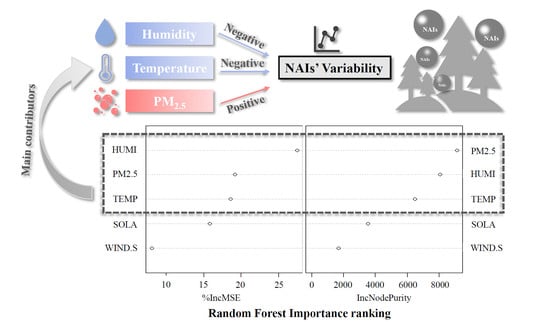
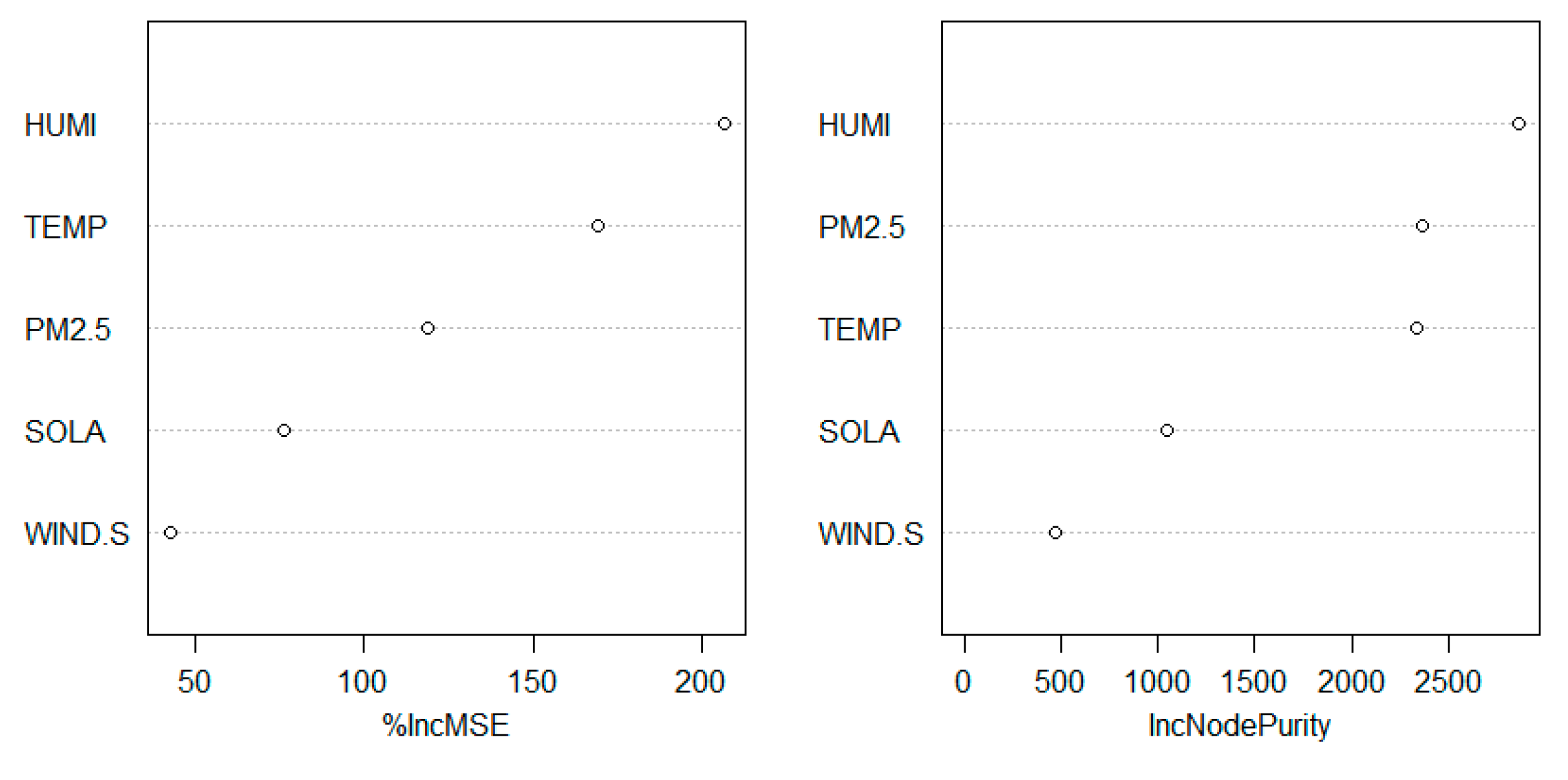
Considering that the RF assessment of the factor group importance was relatively general, we further analyzed and extracted specific typical factor representatives from each factor layer (choosing the factor with the largest coefficient in each factor group) to repeat the importance assessment; we selected TEMP from the phenological factor group, HUMI from the water factor group, SOLA from the radiation factor group, PM
2.5 from the particle matter group, and WIND.S from the wind factor group. NAIVC was then taken as the dependent variable and the remaining factors as independent variables to conduct importance analyses using the RF regression model. The results are given in
Table 5 and
Figure 6.
The results indicate that HUMI is the factor that most strongly affects the variability of NAIs, followed by PM2.5 and TEMP. The two factors exerting the least effect are SOLA and WIND.S. The order of variable importance is HUMI > PM2.5 ≈ TEMP > SOLA > WIND.S.
Remark 2. %IncMSE represents increase mean square error, IncNodePurity represents increased node purity, HUMI represents humidity, TEMP represents temperature, WIND.S represents wind speed and SOLA represents total solar radiation.
4. Discussion
4.1. Influence of Humidity (Water) on NAIV
Pearson correlation analysis, multiple linear regression analysis, and RF analysis all identified humidity as the dominant factor in the variability of NAIs. Correlation analysis revealed humidity to be negatively correlated with NAIVC; multiple linear regression and RF importance analysis indicated that humidity is the most influential factor. We speculate that the reason for this is related to the mechanism for the generation and extinction of NAIs:
The Lenard effect induced by water can promote the formation of NAI [
10].
The molecular formula of NAIs includes O
2(H
2O)
n, OH
−(H
2O)
n, and CO
−4(H
2O)
2. H
2O is seen to be a key factor in the process of NAI generation, and is directly involved in the reaction for NAI generation [
2,
32].
Water droplets in the air have a cleaning effect on atmospheric particulate matter, and this can extend the lifespans of NAIs [
33].
Based on the aforementioned observations, we found that high humidity encourages the generation of NAIs and extends their lifespans, such that the stability of NAIs is improved and the variability of NAIs is subsequently reduced.
In addition, the effects of precipitation are similar to those of humidity. Both affect NAI production through the action of water. However, due to the discontinuity of precipitation data and the lag in data collection, a deviation occurred in the analysis of rainfall, accounting for the underestimation of its importance.
4.2. Influence of Temperature (Phenology) on NAIV
Long-term temperature changes are closely related to phenological changes; temperature is higher during the day than at night and higher during summer than in winter. Moreover, daytime and summer are periods of more vigorous biological activity, and the changes in the roles of NAIs are also much more dramatic. Pressure exerts a negative linear correlation with temperature, and canopy density reflects changes in plants during the year. As in the factor analysis, we unified TEMP, PRES and CD into phenology factors.
Correlation analysis and multiple linear regression both showed that temperature (phenology) is significantly negatively correlated with NAI variability. Higher temperature means greater phenology, which is associated with lower NAIVC; relative weight and RF importance analysis both indicated that the influence of temperature on the NAIC is second only to that of humidity, which is also of major importance. We analyzed the relationship between temperature and NAIV according to the following three aspects:
On a microscopic scale, temperature can affect the rates of NAI generation and extinction reactions; the higher the temperature, the faster the various reactions. From this perspective, temperature can enhance NAI variability.
On the mesoscale, temperature is closely related to many other factors. For example, temperature affects barometric pressure and has a collinear relationship with canopy closure. When temperature is low, air pressure is usually high and canopy density is low, intensifying air circulation and particle collision. Temperature thus has an inverse relationship with NAI variation.
On a macroscopic scale, temperature and phenology are closely connected; the higher the temperature, the more vigorous the phenological activity, and the more intensified the generation of NAIs. As a result, dynamic changes in NAIs are more complicated. Compared to the single mechanism of NAI change, the stability of NAIs is enhanced and variability is reduced.
Overall, the influence of temperature or phenology on the variation of NAIs is complex. Both exert numerous influences that can affect the generation and extinction of NAIs in various manners. Therefore, the role of temperature cannot be overlooked, and its effects vary according to scale. However, from a long-term perspective, the higher the temperature, the lower the NAI variability.
4.3. Influence of PM2.5 on NAIV
For particulate matter, we found that PM
2.5 was significantly positively correlated with NAIV, and PM
10 was the only factor exhibiting no significant correlation. In the RF importance ranking, the influence of PM
2.5 was roughly similar to that of temperature, which also plays a major role in NAIV. We propose that relatively high PM
2.5 concentrations can form aerosols in the air which can collide with and neutralize NAIs and directly affect the extinction process of air ions [
34]; therefore, the higher the concentration of PM
2.5, the faster the death rate of NAIs, reducing the lifespan of NAIs in the atmosphere. Shorter lifetime means greater NAI variability. However, due to larger particle sizes, PM
10 is prone to sedimentation in the air and exerts weak effects on NAIs, and thus, has little influence on the variability of NAIs.
4.4. Influence of Wind and Radiation on NAIV
Among wind factors, wind speed was shown by correlation analysis to exhibit a significant positive correlation with NAIV. The higher the wind speed, the greater the air fluidity; this promotes the migration, collision and extinction of NAIs, thereby increasing variability. In addition, studies have shown that the friction of wind speed can produce NAIs [
35]. Under natural conditions, the wind factor is mutable, and thus, a sudden increase in wind speed may cause an NAIC outburst. The influence of wind direction on NAIs is linked mainly to the location of NAI collection, which demonstrates a high level of randomness. Relative weight and RF importance ranking showed that wind weakly affects NAI variation. A possible reason for this is that wind does not directly participate in the generation and extinction of NAIs. Indirect effects exert relatively little influence. The monitoring site was blocked by a plant community, which means that the air transmission caused by wind was negligible, and thus, that the wind factors are of little importance.
Pearson correlation showed that both total solar radiation and photosynthetic active radiation are positively correlated with negative ion variability. However, an importance analysis indicated that the effect of radiation is also much weaker than the effects of humidity and temperature. The reason for this is that the promotion effect of radiation on NAIs is mostly realized through its influence on the physiological activities of plants, which, similar to wind factors, affect NAI changes only indirectly; thus, they are of low importance.
4.5. Limitations of the Study
In this study, the relationship between NAIV and meteorological factors was discussed for one particular plant community. In urban green spaces, the influences of various plant communities on NAIs are also nonnegligible. Nevertheless, our conclusions reveal that some NAIV characteristics are related to meteorological factors, which can be used to explain why notable differences are present in the results of other NAI research.
The spatial and temporal variation patterns of NAIs are such that meteorological factors, especially humidity, temperature and particulate matter concentration, vary according to region. These factors can directly affect the NAIV, and can also indirectly affect NAIV by controlling other factors. Humidity provides an example of this: High humidity levels exert a significant effect on the stability of NAICs. Therefore, when subject to high-humidity weather, NAIs are not sensitive to changes in temperature and wind speed; however, when humidity is low, the sensitivity of NAIs to wind speed and temperature is enhanced.
Many scholars have also found that under different conditions, the relationship between NAIs and environmental factors differs. For example, Wang et al. found that in Heilongjiang Forest Botanical Garden, the NAIC and PM
2.5 in July exhibited an extremely significant negative correlation, but this was nonsignificant in October [
36]; Xu found that the relationship between NAIs and meteorological factors on sunny, rainy, hazy, and windy days differed notably [
37]; Wang et al. found that there were seasonal differences in the relationship between NAIC and some environmental factors in the Wudalianchi Scenic Area. Therefore, follow-up studies of NAIs require control of meteorological background conditions at the research site or limitation of the range of irrelevant factors in the exploration process to more accurately and effectively understand the characteristics of NAIs.
Based on this study, the selection of green plant species and the planting methods play a key role in maintaining NAIC stably in green spaces. Making a plant community with strong dust-retention ability and vigorous physiological activities such as transpiration and photosynthesis, and setting water features around the community are ways to create a high humidity, low PM2.5 concentration environment where NAICs will not change dramatically.
5. Conclusions
This study used one-year continuous observation data from an urban park plant community to construct an NAI variation index and discussed the relationships of the index values with meteorological factors. We understand NAIV as being derivative of NAIC, and believe that study of the derivative can better reflect the driving force and dominant factors of NAICs. We found water factors, whose main contribution is humidity, and phenology factors, whose main contribution is temperature, to be the most influential factors on the variability of NAIs, followed by particulate factors; wind and radiation factors exerted the least influence. Under natural conditions, high humidity and temperature, and low particulate concentration, can maintain NAICs within a relatively stable range. The reason for this is that high humidity, strong phenology and low-concentrations of particulate matter enrich the paths of NAI production and delay their extinction. The effects of these factors are direct. Wind and radiation exert indirect influences on NAIs, and thus, are of low importance. This study explained the patterns in NAI changes and the influencing factors from the perspective of variability. This deepens our understanding of NAI characteristics and the factors that control them to facilitate better planning and the implementation of conditions which are conducive to the production of NAIs in urban green spaces.
Author Contributions
Conceptualization, L.L. and S.Y.; methodology, L.L. and S.Y.; software, L.L.; validation, L.L., S.Y. and W.S.; formal analysis, L.L.; investigation, L.L., W.S., and W.Z.; resources, C.L. and Y.H.; data curation, L.L.; writing—original draft preparation, L.L.; writing—review and editing, W.S., W.Z. and S.Y.; visualization, L.L. and C.L.; supervision, C.L.; project administration, S.Y. and Y.H.; funding acquisition, S.Y. and Y.H. All authors have read and agreed to the published version of the manuscript.
Funding
This research was co-funded by the National Key Research and Development Program of China (2017 YFC0505501), the National Natural Science Foundation of China (31971719), and Shanghai Landscaping and City Appearance Administrative Bureau (G171206).
Acknowledgments
We appreciate the administration of Zhongshan Park for providing the excellent and typical research sites, and thanks a lot to Ningxiao Sun and Si Miao for their contribution to the data collection work.
Conflicts of Interest
The authors declare that there are no conflicts of interest regarding the publication of this paper.
References
- Krueger, A.P.; Reed, E.J. Biological impact of small air ions. Science (New York, NY) 1976, 193, 1209–1213. [Google Scholar] [CrossRef]
- Lin, H.; Lin, J. Generation and Determination of Negative Air Ions. J. Anal. Test. 2017, 1, 1–6. [Google Scholar] [CrossRef]
- Buckalew, L.W.; Rizzuto, A. Subjective response to negative air ion exposure. Aviat. Space Environ. Med. 1982, 53, 822–823. [Google Scholar]
- Kosenko, E.A.; Kaminsky, Y.G.; Stavrovskaya, I.G.; Sirota, T.V.; Kondrashova, M.N. The stimulatory effect of negative air ions and hydrogen peroxide on the activity of superoxide dismutase. FEBS Lett. 1997, 410, 309–312. [Google Scholar] [CrossRef]
- Watanabe, I.; Noro, H.; Ohtsuka, Y.; Mano, Y.; Agishi, Y. Physical effects of negative air ions in a wet sauna. Int. J. Biometeorol. 1997, 40, 107–112. [Google Scholar] [CrossRef]
- Kellogg, E.W.I. Air ions: Their possible biological significance and effects. J. Bioelectr. 1984, 3, 119–136. [Google Scholar] [CrossRef]
- Seo, K.H.; Mitchell, B.W.; Holt, P.S.; Gast, R.K. Bactericidal effects of negative air ions on airborne and surface Salmonella enteritidis from an artificially generated aerosol. J. Food Prot. 2001, 64, 113–116. [Google Scholar] [CrossRef]
- KRUEGER, A.P.; SMITH, R.F. The biological mechanisms of air ion action. II. Negative air ion effects on the concentration and metabolism of 5-hydroxytryptamine in the mammalian respiratory tract. J. Gen. Physiol. 1960, 44, 269–276. [Google Scholar] [CrossRef]
- Kinne, S. A Public Health Approach to Evaluating the Significance of Air Ions. Master’s Thesis, The University of Texas Health Science Center at Houston, Houston, TX, USA, 1997. [Google Scholar]
- Wu, C.; Zheng, Q.; Zhong, L. Study on the concentration level of negative air ions in forest recreation area. Sci. Silvae Sin. 2001, 05, 75–81. (In Chinese) [Google Scholar]
- Retalis, A.; Nastos, P.; Retalis, D. Study of small ions concentration in the air above Athens, Greece. Atmos. Res. 2009, 91, 219–228. [Google Scholar] [CrossRef]
- Li, J.; Zhang, Y. Characteristic of air negative ion concentration in different ecological functional zones in summer in main urbans of Xinjiang. J. Arid Land Resour. Environ. 2013, 27, 172–176. [Google Scholar]
- Li, S.; Lu, S.; Chen, B.; Pan, Q.; Zhang, Y.; Yang, X. Distribution characteristics and law of negative air ions in typical garden flora areas of Beijing. J. Food Agric. Environ. 2013, 11, 1239–1246. [Google Scholar]
- Zhuo, L.; Liao, C.; Huang, G.; Ma, S. Study on diurnal changing pattern of negative air (Oxygen) ion concentration in Beijing Xishan. For. Resour. Manag. 2016, 02, 110–115. (In Chinese) [Google Scholar]
- Liang, H.; Chen, X.; Yin, J.; Da, L. The spatial-temporal pattern and influencing factors of negative air ions in urban forests, Shanghai, China. J. For. Res. 2014, 25, 847–856. [Google Scholar] [CrossRef]
- Wang, Y.; Ni, Z.; Di, W.; Fan, C.; Lu, J.; Xia, B. Factors influencing the concentration of negative air ions during the year in forests and urban green spaces of the Dapeng Peninsula in Shenzhen, China. J. For. Res. 2019. [Google Scholar] [CrossRef]
- Cong, J.; Sun, L. Establishment of negative air oxygen ion concentration distribution and prediction model in Dalian city. J. Meteorol. Environ. 2010, 26, 44–47. (In Chinese) [Google Scholar]
- Wang, W.; Yu, Z.; Zheng, F. Characteristics of negative air ion concentration and its relationship with environmental factors in various environments in summer. Ecol. Environ. Sci. 2012, 25, 38–40. (In Chinese) [Google Scholar]
- Reiter, R. Part B Frequency distribution of positive and negative small ion concentrations, based on many years’ recordings at two mountain stations located at 740 and 1780 m ASL. Int. J. Biometeorol. 1985, 29, 223–231. [Google Scholar] [CrossRef]
- Pan, J.; Dong, L.; Liao, S.; Qiao, L.; Yan, H. Negative air ion concentration and affecting factors in Beijing Olympic Forest Park. J. Beijing For. Univ. 2011, 33, 59–64. [Google Scholar]
- Huang, S.; Xu, C.; Zhou, J. Path Analysis on Negative Air Ion Concentration and the Meteorological Environment in Urban and Forest Zones. Meteorol. Mon. 2012, 38, 1417–1422. [Google Scholar]
- Huang, X.H.Q.C.; Wang, J.; Zeng, H.; Chen, G.G.C.; Zhong, X. Spatiotemporal distribution of negative air ion concentration in urban area and related affecting factors: A review. Yingyong Shengtai Xuebao 2013, 24, 1761–1768. [Google Scholar]
- China Weather. Available online: http://www.weather.com.cn/ (accessed on 25 June 2020).
- Breiman, L. Random Forests. Mach. Learn. 2001, 45, 5–32. [Google Scholar] [CrossRef]
- Cutler, D.R., Jr.; Edwards, T.C.; Beard, K.H.; Cutler, A.; Hess, K.T. Random forests for classification in ecology. Ecology 2007, 88, 2783–2792. [Google Scholar] [CrossRef] [PubMed]
- Prasad, A.M.; Iverson, L.R.; Liaw, A. Newer classification and regression tree techniques: Bagging and random forests for ecological prediction. Ecosystems 2006, 9, 181–199. [Google Scholar] [CrossRef]
- Uhlenkott, K.; Vink, A.; Kuhn, T.; Martinez Arbizu, P. Predicting meiofauna abundance to define preservation and impact zones in a deep-sea mining context using random forest modelling. J. Appl. Ecol. 2020. [Google Scholar] [CrossRef]
- Wen, L.; Yuan, X. Forecasting CO2 emissions in Chinas commercial department, through BP neural network based on random forest and PSO. Sci. Total Environ. 2020, 718, 137270. [Google Scholar] [CrossRef]
- Miao, S.; Zhang, X.; Han, Y.; Sun, W.; Liu, C.; Yin, S. Random Forest Algorithm for the Relationship between Negative Air Ions and Environmental Factors in an Urban Park. Atmosphere 2018, 9, 463. [Google Scholar] [CrossRef]
- Wang, H.; Wang, B.; Niu, X.; Song, Q.; Li, M.; Luo, Y.; Liang, L.; Du, P.; Peng, W. Study on the change of negative air ion concentration and its influencing factors at different spatio-temporal scales. Glob. Ecol. Conserv. 2020, 23, e01008. [Google Scholar] [CrossRef]
- Archer, K.J.; Kirnes, R.V. Empirical characterization of random forest variable importance measures. Comput. Stat. Data Anal. 2008, 52, 2249–2260. [Google Scholar] [CrossRef]
- Luts, A.; Parts, T.E.; Laakso, L.; Hirsikko, A.; Groenholm, T.; Kulmala, M. Some Air Electricity Phenomena Caused By Waterfalls: Correlative Study of the Spectra. Atmos. Res. 2009, 91, 229–237. [Google Scholar] [CrossRef]
- Chen, H.; Zhang, J. Review on factors influencing the concentration distribution of negative air ions. Ecol. Sci. 2010, 29, 181–185. [Google Scholar]
- Ling, X.; Jayaratne, R.; Morawska, L. Air ion concentrations in various urban outdoor environments. Atmos. Environ. 2010, 44, 2186–2193. [Google Scholar] [CrossRef]
- Wu, Z.; Huang, X.; Huang, C.; Wang, Y. Experimental study on the concentration of negative air ions. J. Xi’an Polytech. Univ. 2007, 06, 803–806. (In Chinese) [Google Scholar]
- Wang, F.; Li, B.; Zhou, Y. Relationship between the Negative Air Ion Concentration and the Meteorological Factors in the Urban Forest Park. J. North-East For. Univ. 2016, 44, 18. [Google Scholar]
- Xu, L. Spatial-Temporal Variation Characteristics and Influencing Factors of Urban Forest Air Negative Ion Concentration in Beijing. Master’s Thesis, Shenyang Agricultural University, Shenyang, China, 2019. (In Chinese). [Google Scholar]
© 2020 by the authors. Licensee MDPI, Basel, Switzerland. This article is an open access article distributed under the terms and conditions of the Creative Commons Attribution (CC BY) license (http://creativecommons.org/licenses/by/4.0/).


