Article

Alpine Tundra Contraction under Future Warming Scenarios in Europe

1
European Commission, Joint Research Centre, 21027 Ispra, Italy
2
Arcadia SIT s.r.l., 27029 Vigevano, Italy
*
Author to whom correspondence should be addressed.
Atmosphere 2020, 11(7), 698; https://doi.org/10.3390/atmos11070698
Submission received: 6 May 2020 / Revised: 22 June 2020 / Accepted: 25 June 2020 / Published: 1 July 2020
(This article belongs to the Special Issue Impact of Climate and Land-Use Change on the Earth’s Critical Zone)

Abstract

:
The alpine tundra is the highest elevation belt of high mountains. This zone is an important reservoir of freshwater and provides habitat to unique species. This study assesses projected changes in the areal extent of the alpine tundra climate zone in three warming levels in European mountains. The alpine tundra was delineated using the Köppen-Geiger climate classification. We used 11 regional climate model simulations from EURO-CORDEX disaggregated at a one-kilometre grid size representing the RCP4.5 and RCP8.5 scenarios in the 1.5, 2 and 3 °C warming levels. Mitigation represented by the 1.5 °C warming level reduces projected losses of the alpine tundra. However, even in this warming level the projected contraction is severe. In this case, the contraction in the Alps, Scandes and Pyrenees together is projected at between 44% and 48% of the present extent. The contraction is projected to climb in the 2 °C warming to above 57%, while the 3 °C warming would imply that the alpine tundra will be near to collapse in Europe with a contraction of 84% in the three regions, which host most of the alpine tundra in Europe. The projected changes have negative implications for a range of ecosystem services and biodiversity, such as habitat provision, water provision and regulation, erosion protection, water quality and recreational services.

1. Introduction

High mountain ecosystems provide vital services to humans, such as freshwater, water regulation and release during the drier summer months from melting snow, habitat for biodiversity, and recreational services. High mountains are characterised by a cold and harsh climate, high altitudes and complex topography. Forest and grasslands often cover the lower slopes, but at higher elevations trees become scarcer, giving place to alpine grasslands and scrub heath communities. Due to their steep gradients, mountains comprise latitudinal life zones in a relatively small extent, therefore habitats and species change rapidly with altitude. These characteristics explain the rich biodiversity and variety of habitats present in mountain regions. For instance, two thirds of European plant species are present in mountains [1,2].
Anthropogenic climate change presents a major threat to mountain systems. Due to the tight ecological-climatic bands in mountains, small changes could have major effects in these systems. There is consensus that alpine habitats are showing a high sensitivity to climate change and will be highly vulnerable to future changes [3,4]. Evidence indicates that in mountain regions the current and future effects of global warming are likely to be amplified [4,5,6,7,8,9,10,11,12]. Therefore, projected climate-driven impacts are greater at higher elevations [13,14].
In Europe, alpine tundra occurs at the top of high mountains above the tree line ecotone, where alpine grasslands and scrub heath communities dominate vegetation. The climate of the alpine tundra does not support tree growth [15]. The nival zone is at the top of the alpine tundra, where snow is present most of the year. The Alpine tundra is an important reservoir of freshwater resources and play a key role in water release. Mountain ecosystems intercept water and store it as snow, glaciers and reservoirs before delivering mostly in spring and summer. These ecosystems play a key role in water provision for agriculture and human consumption and provide key ecosystem services such as habitat to endemic species and alpine communities.
Alpine tundra is present across Europe in several high elevation mountains. The most extended zones are the high mountain ranges of the Pyrenees on the border between France and Spain; the Alps, which stretch over France, Italy, Germany, Austria, Slovenia, Switzerland and Monaco; the Scandes located between Sweden, Norway and Finland; and some less prominent zones, such as the Scottish Highlands and Carpathians.
The impacts of climate change in high mountain areas have been a subject of intensive research in the last two decades. The Intergovernmental Panel on Climate Change’s (IPCC’s) Special Report on Ocean and Cryosphere in a Changing Climate presents a comprehensive summary of available findings [4]. Among the observed and projected changes in high mountains, the most notable are the shrinking of glaciers [16,17], reductions in snow cover [7], increased permafrost temperature [18], shifts in ranges of plant and animal species [10,11,14,19,20,21], and effects in ecosystem functions [22]. Nevertheless, the potential impact of climate change in the extent of the alpine tundra climate zone is poorly understood. Therefore, better knowledge on this impact is necessary for appropriate adaptation in alpine ecosystems. The aim of this study is to assess changes in the extent and distribution of the alpine tundra climate in Europe under scenarios of climate change. Additionally, we discuss potential impacts on biodiversity, ecosystem services, hydrology, and slope dynamics from available evidence.
The results of this study are useful for mapping critical conservation areas and support decision making on potential interventions, such as Green Infrastructure [23], and other adaptation options in high mountain ecosystems.

2. Methods

In this study, we mapped the European alpine tundra climate zone under historical climate (reference period 1981–2010), and two Representative Concentration Pathways (RCPs) adopted by the Intergovernmental Panel on Climate Change (IPCC) in its Fifth Assessment report, specifically RCP4.5 and RCP8.5 [24,25]. RCP4.5 is a trajectory projecting an increase in global mean temperature of 1.8 °C (likely range 1.1–2.6 °C) relative to the period of 1986–2005 [26]. While RCP8.5 is a business as usual (high emission) trajectory [24,25], projecting a + 3.7 °C (likely range 2.6–4.8 °C) world by the end of the century relative to 1986–2005 [26].
We used 11 Regional Climate Model (RCM) simulations for three warming levels, i.e., 1.5, 2 and 3 °C, the latter reached only in RCP8.5. The warming levels represent 30-year periods centred on the year when the driving general circulation model (GCM) projects a global 1.5, 2 and 3 °C warming, with respect to pre-industrial levels, according to the IMPACT2C [27] project. See the simulations used and the 30-year time ranges in Table 1. Maps accounting for changes in the alpine tundra were created for the 11 simulations, two scenarios and three periods.
This study was implemented within the PESETA IV project [28], which aims at evaluating potential impact of climate change in Europe for a number of sectors. A common set of climate simulations and scenarios were used by all sectors with a focus on the biophysical dimension of impacts, extreme events and the exploration of various adaptation options. Therefore, the baseline period, scenarios, warming levels and simulations were selected according to the project guidance.

2.1. Climate Data

We obtained high-resolution RCM simulations from the Coordinated Regional Downscaling Experiment (CORDEX) of the World Climate Research Programme (WCRP). The EURO-CORDEX [29] initiative provides regional climate projections for Europe at ~12.5 km horizontal resolution by downscaling the global climate projections of the Coupled Model Intercomparison Project Phase 5 (CMIP5) [30]. We used simulations of daily air temperature for 11 RCMs, 2 RCP scenarios and 4 periods (reference period, 1.5, 2 and 3 °C warming levels). Departing from daily data, we calculated 30-year monthly mean air temperature data sets. The spatial domain of this study covers the EU-28, Switzerland and Norway.
Given that the alpine tundra biome is located in high mountain areas, and that these are characterised by complex topography and large elevational gradients, using RCM simulations at a ~12.5-km horizontal resolution for mapping alpine tundra is problematic. This is because horizontal variations in temperature in high mountain areas cannot be captured properly at the resolution of RCMs [31]. Aimed at alleviating this limitation we used the change factor approach for reduce model bias and spatially disaggregate temperature fields from RCMs to a higher horizontal resolution of 1 km [31,32,33,34,35]. The resulting high resolution data set is appropriate for high mountain and biodiversity studies [31,36].
Anomalies (differences) of monthly mean temperature were computed from the RCM future simulations (1.5, 2 and 3 °C warming levels) and the reference period (1981–2010). Then, temperature anomalies were interpolated using the spline method [37,38] to the 1-km spatial resolution of the baseline data, i.e., CHELSA ver. 1.2 [39]. We used the regularised spline with a weight of 0.001 and 8 points. These parameters are well suited for the interpolation of RCM data according to Barredo et al. [33]. Finally, temperature anomalies were added to the corresponding month of the CHELSA dataset for producing high-resolution maps of future monthly mean air temperature. The CHELSA dataset, which covers the period 1979–2013, approximates the reference period of this study, which was agreed in the PESETA IV Project.

2.2. Mapping Alpine Tundra Domain

Alpine tundra was mapped using the Köppen-Geiger climate classification [40] following the work of Diaz and Eischeid [6] and Kottek, et al. [41]. The alpine tundra domain (ATD) is equivalent to the polar climates classified in Köppen-Geiger as E-type [6]. Polar climates are defined as occurring if the mean temperature of the warmest month is less than 10 °C. These include two Köppen-Geiger sub-types, i.e., tundra climate (ET) and frost climate (EF). Tundra climate occurs where the mean temperature of the warmest month is in the range of less than 10 and 0 °C, and frost climate occurs where the mean temperature of the warmest month is less than 0 °C. No precipitation differentiation is included in the Köppen-Geiger classification for these two sub-types. The EF sub-type is present in the study domain in a few marginal areas. Therefore, we defined the ATD as equivalent of polar climates (E-type) according to Diaz and Eischeid [6]. This analysis focuses on climatic impacts and maps the ATD based solely on climatic criteria.
Maps of the ATD were created for the reference period and for each scenario, period and simulation. Thus, in addition to the map of the reference period created using CHELSA, we obtained 33 maps (11 simulations times 3 periods) for RCP8.5 and 22 maps (11 simulations times 2 periods) for RCP4.5.
Then, summary maps describing changes in the ATD containing three potential categories (stable, contraction and expansion areas) were created between the reference period and the future. As a result, we obtained one map of projected changes for each scenario/period. The category expansion is absent in the summary maps and was therefore excluded from the assessment. The maps were summarised according to Table 2 following Klausmeyer and Shaw [34]. Therefore, the number of simulations predicting changes of the ATD (stable or contraction) was used to define the category of change on each grid cell.
For example, if only six simulations project that a grid cell will remain within the ATD in the 3 °C warming level, then that grid cell is included in the uncertain category in the mentioned warming level. Similarly, if 10 simulations project that a grid cell will remain within the ATD in the 3 °C warming level, then that grid cell is included in the stable category in the mentioned warming level. We used equal-area projected maps for computing areal changes, taking the curvature of the earth into consideration.

2.3. Validation of the Alpine Tundra Delineation

We implemented a validation procedure to determine the ability of our methodology to reproduce a faithful delineation of the ATD using an independent map of the alpine tundra biome. However, lack of independent pan-European maps of alpine tundra with sufficient spatial detail to allow a fair comparison with the ATD makes the validation challenging.
Beside the very coarse maps of tundra biomes available, e.g., [42,43,44], to the best of our knowledge, the only map representing the alpine tundra biome is the Map of the Natural Vegetation of Europe of Bohn et al. [45]. The map of natural vegetation is well suited for comparison because it represents the potential distribution of vegetation in Europe that is the vegetation that would occur without human intervention. This is similar to the climatic approach used in this study, where other effects beyond climate are not taken into account for mapping the ATD. There is controversy regarding the map of Bohn et al. [45] because it is not based on a quantitative analysis but on expert knowledge. However, the map has proven to be robust in recent applications of simulated vegetation distribution in Europe [46] and the degree of naturalness of European forests [47].
In the validation, we used a map of the ATD created using WorldClim data (Version 1.4) at a one-kilometre grid size [48] instead of the CHELSA dataset. This is because the reference period of WorldClim v1.4 (1960–1990) is in agreement with the map of Bohn et al. [45], which refers to around the same period. The validation is aimed to assess the capacity of the method for mapping the ATD, independently of the climate data set used.
We assumed that the ATD approximates the alpine tundra biome represented by the subunits subnival vegetation of high mountains (A.2), alpine vegetation (B.2) and glaciers as described in the Map of the Natural Vegetation of Europe [45]. The alpine vegetation formation includes alpine grasslands, low creeping shrub, dwarf shrub and shrub vegetation, rock and scree vegetation. These subunits occur above the tree line in high mountain regions, where trees are completely absent, similarly as in the ATD.
For the comparison, the biome map was cropped to the extent of the ATD map. Then, we calculated a buffer of five kilometres from the alpine tundra categories of the two maps to avoid that a large number of background grid cells are counted as agreement, therefore biasing the validation towards agreement. As result, we obtained two binary maps where grid cells with 1 represents the ATD and alpine tundra biome, respectively, in both maps, and grid cells with 0 the background within the five kilometres buffer. The validation was implemented independently in three mountain regions, i.e., Alps, Scandes and Pyrenees.
The level of agreement between the maps generated was assessed using the Kappa statistic [49,50] and overall accuracy [51]. The Kappa statistic measures the degree of agreement between categorical maps, ranging from zero (total disagreement) to one (perfect agreement) [52]. Overall accuracy is a simple technique for map comparison. It is computed by dividing the number of coincident grid cells by the total number of grid cells.

2.4. Sensitivity Analysis

A sensitivity analysis was carried out to assess the level of agreement between the different simulations in mapping projected losses of the ATD. We computed projected areal losses of the ATD relative to the reference period using the maps of the ATD for the different combinations of scenarios and warming levels. Then, projected losses, i.e., areas where the ATD is projected to disappear, were represented in box-and-whisker plots per region, scenario and warming level for comparison.

2.5. Climate Parameters

The projected changes in climate parameters were computed for both scenarios and the three warming levels in the ATD. We computed changes of mean monthly temperature and mean monthly precipitation in the summer half of the year (April to September), winter half of the year (October to March) and annually. In addition, the temperature of the warmest month of the year was also computed because it is the parameter defining the ATD. We computed the changes within the ATD delimited in the map of the reference period.

3. Results

In Europe (excluding Iceland), the extent of the ATD in the reference period is around 87,000 km2. This is close to the size of Austria or Portugal. Of this extent, 98% is found in the Alps, Scandes and Pyrenees, representing around 25,000 km2, 59,200 km2 and 1800 km2, respectively (Figure 1). A few isolated areas of ATD are present in the Scottish Highlands, Tatra Mountains, Carpathians and Apennines in central Italy.

3.1. Validation of Alpine Tundra Delineation

Despite differences in the methodology for mapping alpine tundra between the climatic approach used in this study and the expert knowledge approach used in the map of Bohn et al. [45], the results of the validation indicates a level of agreement above 70% between both maps (Table 3). A commonly cited interpretation of the Kappa statistic suggests slight agreement in the range 0.01–0.20, fair agreement 0.21–0.40, moderate agreement 0.41–0.60, substantial agreement 0.61–0.80 and almost perfect agreement 0.81–0.99 [52].
The match is moderate in the Alps and Pyrenees where Kappa and overall accuracy are above 0.42 and 78%, respectively. The maps in Figure 2 reveal that the delineation of the ATD is more restrictive than the subunits delineated in the alpine tundra biome map in the Alps and Pyrenees. There is agreement between the higher elevation zones of the ATD and the categories subnival vegetation of high mountains, glaciers, and the alpine vegetation (at the higher elevations) of the alpine tundra biome map. In contrast, some expanses of the alpine tundra biome at lower elevations fall outside the area delimited by the ATD. This mismatch at lower elevations occurs marginally in the Pyrenees.
Both maps are fairly in correspondence in the Scandes, showing a Kappa statistic and overall accuracy of 0.40 and 70%, respectively. There is more agreement in the southern region of the Scandes, specifically at higher elevations, where the ATD and the alpine tundra biome are in correspondence. Similarly, as in the other two regions, some lower elevation zones of the alpine tundra biome fall outside the ATD. In the northernmost region of the Scandes, the alpine vegetation category of the alpine tundra biome map is delineated further south and east with respect to the ATD (Figure 2). Therefore, pushing down both the Kappa statistic and overall accuracy.
Bohn et al. [45] indicated that the vegetation above the tree line in Scandinavian mountains is considered part of the category alpine vegetation (B.2). However, the alpine vegetation (B.2) resembles the adjacent Arctic shrub tundras (B.1.4), showing a continuous transition zone in the norther boreal region. This makes challenging delineating their limit as there is no discontinuity between them in this region. For instance, a narrow strip of land in the northernmost part of Norway delineated in Bohn et al. [45] as Arctic shrub tundras (B.1.4) and therefore not included in the map of the alpine tundra biome falls almost entirely in the ATD. The mentioned strip of land includes the northernmost part of the Varanger Peninsula, a narrow strip in the north of the Nordkinn Peninsula and the Magerøya Island.
Some areas of the ATD fall outside the limit of the alpine tundra biome in the three regions. The reasons behind this discrepancy have yet to be elucidated. However, it is possible that the coarse scale of the biome map might have played a role in this case.
In general, the ATD resembles the delineation of the alpine tundra biome. However, at lower elevations, the subunit alpine vegetation of the biome map covers an extent somewhat beyond the lower elevational boundary of the ATD. One factor that could explains this difference is that the lower limit of the alpine vegetation subunit borders with the tree-line ecotone, which is a transition zone between the alpine tundra and subalpine forests. Despite these constraints, and considering the rather different methods used for producing the maps and the coarse spatial resolution of the biome map, the validation shows spatial agreement between the delineation of the ATD and the alpine tundra biome.

3.2. Sensitivity Analysis

The results of the sensitivity analysis reveal agreement among the simulations. That is, all the RCM simulations projected contraction of the ATD across scenarios and warming levels. As expected, the projected loss of the ATD is less pronounced in 1.5 °C warming and losses increase with warming level (Figure 3). Nevertheless, the magnitude of the projected contractions of the ATD vary between the 11 simulations. For example, under RCP4.5 in the 1.5 °C warming in the Alps the contraction is projected at between 21% and 49%, that is, the minimum and maximum contraction projected by the 11 simulations, respectively, with respect to the extent in the reference period. In this case, the projected median contraction of the 11 simulations is 34%.
The projected contraction of ATD vary considerably depending on the region considered. For instance, in the 1.5 °C warming level, the projected median loss is around 80% in the Pyrenees and above 47% in the Scandes. While the projected mean contraction in the Alps is less pronounced, though still representing 34–40% of the extent in the reference period. Moreover, in the 2 and 3 °C warming levels, the simulations project losses of different magnitude across regions. In the 2 °C warming level, the mean contraction is projected in the range of around 54%, 63% and above 90% in the Alps, Scandes and Pyrenees, respectively. Finally, in the 3 °C warming level the projected mean contraction is around 76% and 88% in the Alps and Scandes, respectively. While in the Pyrenees the mean contraction across simulations is projected at 99% of the current extent. In other words, the mean contraction of the 11 simulations indicates that the ATD is projected to virtually disappear in this region.

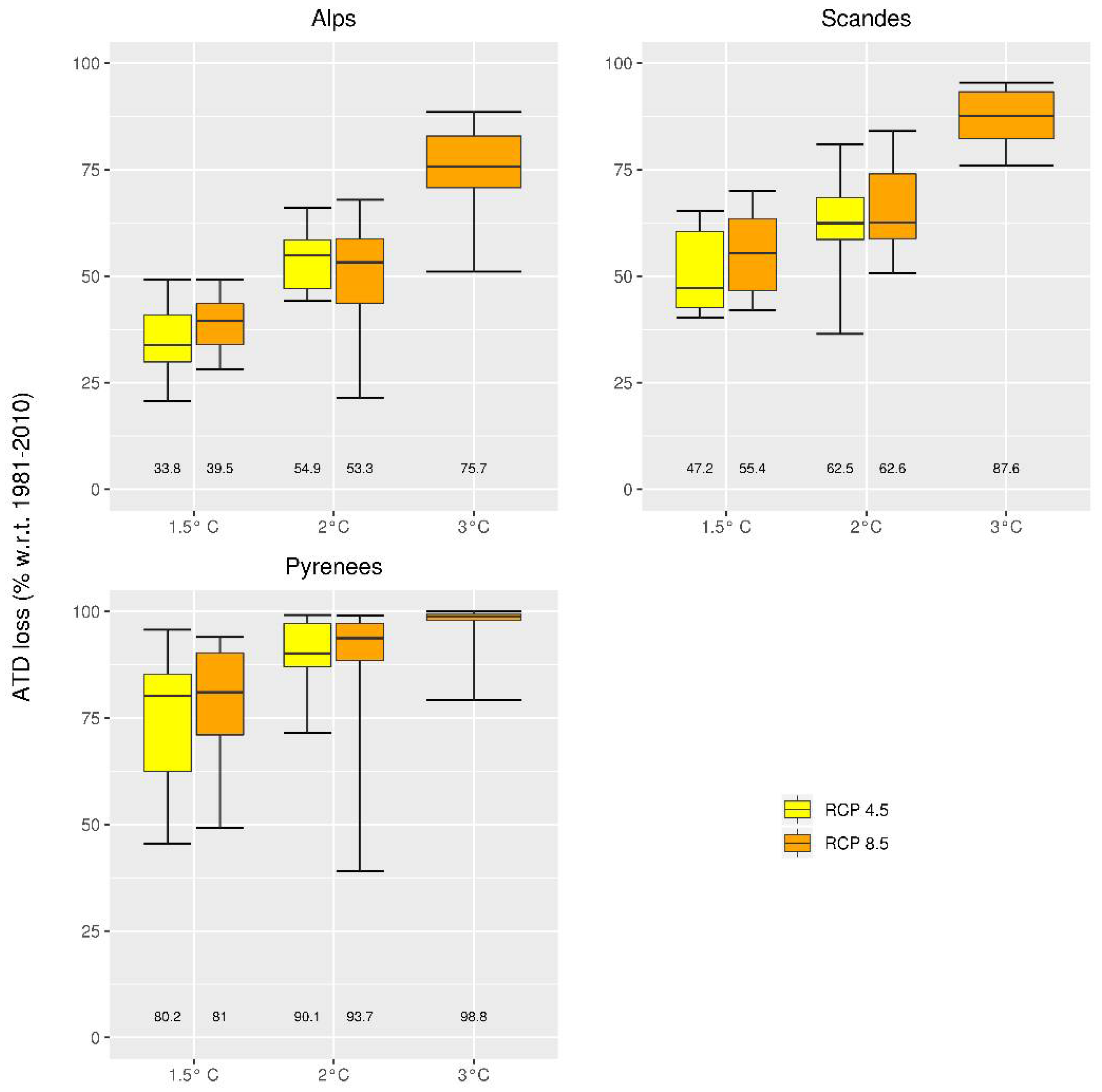
3.3. Mapping Projected Changes of the Alpine Tundra

The results of this study indicate a pronounced projected contraction of the ATD across regions, scenarios and warming levels (Table 4 and Figure 4). In the Alps, it is projected that the ATD will lose an extent of around 31–36% of the current area with a 1.5 °C warming, exhibiting both RCP scenarios similar results (Figure 5). Note that in this section we report changes including both the likely and confident categories unless mentioned otherwise. The projected loss is more pronounced in lower areas, particularly in the eastern and southwestern Alps where the mountain range rarely goes beyond 2600 m a.s.l. Then, in a 2 °C warming, the ATD is projected to lose around half of their extent in this region. While in the 3 °C warming the losses are projected at 75%. Therefore, the extent of the ATD in the Alps is projected to be only 19% of their present area. The remaining 6% is part of uncertain changes (Figure 4). Consequently, almost the entirety of ATD areas below 3000 m a.s.l. are projected to disappear.
In the Scandes, a contraction of the ATD of around half of the present extent is projected in the 1.5 °C warming level in both scenarios (Figure 6). In the 2 °C warming level, a contraction of around 60% is projected in either scenario. The shrinking is particularly pronounced in the northern Scandes, with the ATD persisting only in the highest mountain ranges. In the southern Scandes, the contraction is less severe due to the presence of higher mountain ranges above 1800 m a.s.l., which may act as refugia for alpine tundra biota. Then, in the 3 °C warming level, 87% of the ATD is projected to disappear and only 8% is projected to persist. The remaining 5% falls in the uncertain category.
In the Pyrenees, the projected contractions of ATD are more pronounced than in the Alps and Scandes. In this region, the shrinking is already above 74% in the 1.5 °C warming level in both scenarios (Figure 7). In the 2 °C warming level, the projected contraction is above 90%, making that only around 4% of the ATD is projected to persist, whereas the ATD is projected to virtually disappear in a 3 °C warming level in the Pyrenees.
Our findings indicate that both scenarios, RCP4.5 and RCP8.5, project comparable results across regions regarding the 1.5 and 2 °C warming levels, as illustrated by Figure 4. Results describing changes in climate parameters are in Appendix A.

4. Discussion

We assessed the contraction of the alpine tundra using an approach that accounts for changes in the area of analogous climates. The results of this study indicate that projected increases in the mean temperature of the warmest month, the parameter defining the ATD, drive a pronounced contraction of the alpine tundra climate zone across European mountains.
The magnitude of contraction is smaller at lower warming levels. For instance, in a 1.5 °C warming, the contraction in the Alps, Scandes and Pyrenees together is projected at between 44% and 48% of the present extent, which is equivalent to a contraction of around between 37,000 km2 and 41,000 km2 out of 86,000 km2 in the reference period. The contraction is projected to climb in the 2 °C warming to above 57% or around 49,000 km2. Lastly, under a 3 °C warming, the projected loss in the three regions is 84% of the present extent, or around 72,000 km2.
Our results indicate that the RCP4.5 and RCP8.5 scenarios project a comparable contraction of the ATD under the 1.5 and 2 °C warming levels. This finding is consistent with previous evidence indicating that the effect of the RCP to reach a global warming level is negligible over Europe if compared to the internal variability in the time period involved in reaching the warming level [53]. Nevertheless, a warming of either 1.5 or 2 °C is projected to occur earlier in RCP8.5 than in RCP4.5 because these scenarios follow different trajectories of greenhouse gases concentrations (Table 1). This has implications for adaptation and mitigation because a trajectory following RCP8.5 will shorten the time response to implement adaptation and mitigation actions.
As expected, the contraction of the ATD is projected to occur first at lower elevations. That is, the lower elevational boundary of the ATD zone, where the mean temperature of the warmest month of the year is just below 10 °C. This is evidenced in the maps of ATD change under 1.5 °C warming in Figure 5, Figure 6 and Figure 7. Then, the contraction climbs to higher elevational belts under the 2 and 3 °C warming. A notable feature is that the fragmented nature of the ATD increases further at higher warming levels. This opens questions regarding the persistence of small patches of ATD in the future.
In this study we have focused on the alpine tundra, as defined by a single climatic metric. Nevertheless, the contraction of the ATD domain is consistent with a range of documented and projected environmental effects, such as changes in species diversity and composition and the function of high-altitude mountains ecosystems. However, despite the great importance of the potential impacts of a temperature increase in mountain systems, our understanding of the processes involved is limited [22].
Reductions in the areal extent of the ATD can have an important impact on ecosystem functions and consequently on its services [54]. For example, regarding water provision, winter snowpack accumulation and snow retention in summer occurs in the highest belts of mountains’ environments, associated with the ATD. The retention of snow is critical because it releases water from the mountains during the summer months. Therefore, the contraction of the ATD is consistent with reductions in snowpack, affecting, therefore, low elevation biota and changing mountain hydrology [4,16,55]. A declining snow cover and ice reservoir will prolong periods of low river flow in summer in many parts of Europe. This can have negative consequences in several economic sectors including agriculture, hydropower generation, water supply and river navigation [4,56].
Shrinks of the ATD support evidence of warming-driven changes in alpine plant assemblages that suggest a decline in cold-adapted species and the increase in more warm-adapted species. This process suggests a progressive decline of cold mountain habitats and their associated biota [10,11,54]. Nevertheless, there is great uncertainty regarding potential impacts in plants diversity in mountain systems [22,57], and there is controversy regarding whether the impacts of climate change will be negative in absolute terms or there could be beneficial aspects as well [58,59]. For instance, Engler et al. [14] suggest that 36–55% of alpine plant species will lose more than 80% of their suitable habitat by the end of the century in Europe. In contrast, Rixen and Wipf [60] indicate that the extinction of high mountain plants may be mitigated by the high diversity of microhabitats, the longevity of alpine plants and positive plant–plant interactions in harsh environments.
One of the most notable impacts of warming, consistent with ATD contraction, is the pervasive shrink of glaciers [4,16,17]. Rapid changes in glaciers result in multiple impacts in social-ecological systems, including formation of ice-marginal lakes, ice avalanches and mass movements [61,62], runoff volume and sediment fluxes. Observational evidence indicates a consistent reduction in glacier mass across mountains at global level, with the Alps and Pyrenees among the most affected zones [4,16].
Our assessment is consistent with previous studies that have demonstrated that warming will affect notably high mountain environments in Europe. For instance, our results are in accordance with a previous study assessing the changes of Köppen-Geiger climate zones in the Alps. Rubel et al. [30] assessed observational and future changes using projections from a single RCM and end-of-century RCP2.6 and RCP8.5 scenarios disaggregated at 30 arc-seconds (~1 km), which is the same horizontal resolution used in our assessment. They used simulations from the RC4 RCM with boundary conditions from the EC Earth model that is one of the 11 RCM models included in our assessment (see Table 1). However, a direct comparison between both studies is not straightforward because Rubel et al. [30] assessed impacts by the end of the century, while we assessed changes in relation to warming levels that are projected to occur earlier. For example, the range of the 3 °C warming in the 11 simulations falls between 2037 and 2084, while the 1.5 and 2 °C warming levels are projected to occur earlier (see Table 1). Rubel et al. [30] indicate that by the 2076–2100 the alpine tundra in the Alps will be constrained into small areas under RCP2.6 and is projected to disappear almost entirely under RCP8.5. These findings are consistent with our results that projected a contraction of around 75% of the ATD in the Alps in the 3 °C under RCP8.5.
Numerous studies on cryogenic changes indicate that snow cover, glaciers and permafrost are projected to continue decline in European high mountains throughout this century [4]. As in the case of the ATD, changes in glaciers are triggered primarily by atmospheric conditions. Hock et al. [63] concluded that projected changes indicate that glaciers in European mountains will lose more than 75% of their current mass by the end of the century under RCP8.5 [4,63]. The Alps and Pyrenees will be among the most affected zones exceeding 80%. Similarly, the losses in Scandinavian glaciers are projected over 75% in the same scenario. In the study of Hock et al. [63], changes under RCP4.5 do not diverge substantially from RCP8.5. Another study indicated that glaciers in the European Alps will virtually disappear by 2100, projecting mass losses above 94% under RCP8.5 and above 63% under the low emissions RCP2.6 [64].
Despite the fact that most studies assessed changes by the end of the century, in contrast to our study that assessed changes earlier, and that glacier mass loss and ATD contraction are driven by different factors, the projected changes of these two processes are in accordance with each other. Similarities in the magnitude of the projected changes are reasonable considering that glaciers fall entirely in the area delineated by the ATD (not shown), and that the contraction of this domain seems consistent with glacier area and mass reduction.
We presented a transparent methodology for mapping changes in the alpine tundra climate zone. Nevertheless, in addition to uncertainties in climate models, there may be some possible limitations in this study. For instance, despite the fact that we used state-of-the-art RCM simulations, their horizontal resolution might be coarser than then optimal resolution for assessments in high mountains. We alleviated this issue by using the change factor downscaling method. This method captures only the signal of change from climate models with no further local detail. However, when used with input from RCMs provides suitable data for regions with complex topography [31].
The CHELSA climate data used in the reference period is a valuable data set for continental and global studies. Nevertheless, the one kilometre horizontal resolution of CHELSA might be coarser than the high horizontal resolution necessary to map microclimate zones [65,66]. For example, the Varanger Peninsula, in the northeasternmost part of Norway, that would be part of the ATD according to the national-level maps of Tveito et al. [67], falls partially outside the ATD using CHELSA or WorldClim.
Another limitation concerns the validation data set. A data set delineating the European domain of the alpine tundra at a high spatial resolution is, to our knowledge, not available. Therefore, we used a set of categories of the Map of Natural Vegetation of Europe for delineating the alpine tundra biome. This map presents some constraints because it is based on expert knowledge. Despite this, the alpine tundra biome map proved to be effective in the validation
Using the full ensemble of the CMIP5 simulations would give a better representation of uncertainty in the future climate than the set of 11 RCM simulations used. Despite this limitation, Dosio [68] demonstrated that the range of the 11 RCM simulations for a selection of climate change indices is in accordance, over Europe, with the range produced using the full CMIP5 ensemble by Sillmann et al. [69].
The extent of the alpine tundra habitat is the product of the action of biotic and abiotic drivers. Therefore, future changes in this habitat will be the result of these drivers and its interactions. Instead, our method to delineate the ATD is based solely on climatic factors and no other drivers.
The approach used for delineating the ATD is based in one temperature metric. This is because the Köppen-Geiger classification disregards a precipitation limit for delineating the alpine tundra as moisture shortages are, in general, not characteristic of high elevations. This is in agreement with Körner [15] and Körner and Paulsen [70] that found that a temperature threshold is the unique predictor of the tree line altitude, which occurs just below the alpine tundra. Our study indicates that mean annual precipitation is projected to increase in the ATD of the Alps and Scandes (Figure A2 in Appendix A) and to decrease in the Pyrenees between less of 1% and 8%, across scenarios and warming levels, in relation to the 1207 mm/year of the reference period. This decrease results in a projected precipitation well above, for example, the 200–250 mm/year that is considered the limit for tree grow at the highest elevations [15].
Assessing habitat exposure to climate change is challenging, and, actually, the multiple dimensions of exposure can be represented by different metrics. In this study, we used one metric that accounts for areal changes of the ATD. Assessments using more types of metrics could convey complementary information regarding the potential impacts of climate change on species, habitats and biodiversity. An example is the use of species distribution models with RCM data [71].
The ATD is projected to face a pronounced contraction in Europe, resulting from increased temperatures. The shrinking of this domain is associated with a range of impacts in high mountain ecosystems. Including habitat degradation and biodiversity loss, changes in mountain hydrology, increased natural hazards and significant negative effects in recreational ecosystem services, among others. Therefore, ecosystem-based adaptation efforts should be oriented to protect and restore key sensible habitats and species. Nevertheless, adaptation options in high mountain environments face a number of constraints arising from their unique topographic, edaphic and climatic characteristics [3,72]. In addition, the unprecedented projected changes open research challenges that should be addressed before we can fully understand if and how humans can implement conservation options in alpine areas to prevent, for instance, extinction of alpine species [60].
Impacts and adaptation challenges increase with warming level. Similarly, mitigation, as represented by the 1.5 °C warming, reduces projected losses of the alpine tundra. However, even in this case the contraction of the alpine tundra and concomitant effects in mountain systems would be severe. The effects are projected to increase in the 2 °C warming, while the 3 °C warming would imply that the alpine tundra will be near to collapse in Europe.

Author Contributions

All authors contributed to the preparation of the paper. Conceptualization, J.I.B., A.M. and G.C.; Data curation, J.I.B., A.M. and G.C.; Formal analysis, J.I.B., A.M. and G.C.; Funding acquisition, J.I.B.; Investigation, A.M. and G.C.; Methodology, J.I.B., A.M. and G.C.; Project administration, J.I.B.; Resources, J.I.B.; Supervision, J.I.B.; Validation, J.I.B., A.M. and G.C.; Visualization, J.I.B., A.M. and G.C.; Writing–original draft, J.I.B.; Writing–review & editing, J.I.B., A.M. and G.C. All authors have read and agreed to the published version of the manuscript.

Funding

This research received funding from the PESETA IV Project “Climate impacts and adaptation in Europe”, European Commission, DG-CLIMA.

Acknowledgments

The authors acknowledge the EURO-CORDEX initiative for providing the climate simulations obtained from the Earth System Grid Federation server. We are grateful to all the modelling groups that performed the simulations and made their data available, namely, Laboratoire des Sciences du Climat et de l’Environnement (IPSL), Institut National de l’Environnement Industriel et des Risques, Verneuil en Halatte (INERIS), the CLM community (CLMcom), the Danish Meteorological Institute (DMI), the Royal Netherlands Meteorological Institute (KNMI), and the Rossby Centre, Swedish Meteorological and Hydrological Institute (SMHI). We also thank the CHELSA (Climatologies at high resolution for the earth’s land surface areas) and WorldClim initiatives for providing the baseline climate data sets. The authors would like to thank two anonymous reviewers who have provided helpful comments on the refinement of the paper. The views expressed in this article are those of the authors and do not necessarily reflect an official position of the European Commission.

Conflicts of Interest

The authors declare no conflict of interest. The funders had no role in the design of the study; in the collection, analyses, or interpretation of data; in the writing of the manuscript, or in the decision to publish the results.

Appendix A. Climate Parameters

Changes in climate parameters indicate that the area of the ATD is projected to be warmer across regions, whereas projected changes in precipitation are less homogeneous, indicating a wetter climate in the Alps and Scandes and a drier climate in the Pyrenees. Temperature is projected to increase in winter and summer across scenarios, warming levels and regions (Figure A1). In the Alps and Scandes, the increase is more pronounced in winter, in contrast to the Pyrenees where the increase is greater in summer. Thus, the mean annual temperature is projected to increase from the current −1.3, −1.8 and 0.6 °C in the Alps, Scandes and Pyrenees, respectively, to 0.2, 0 and 2.3 °C in the 2 °C warming level. Comparable results between RCP4.5 and RCP8.5 are projected in the 1.5 and 2 °C warming levels. In the 3 °C warming level, the mean annual temperature is projected to almost double the increase projected in the 2 °C warming, thus projecting temperatures at 1.5, 1.2 and 3.6 °C in the three regions, respectively (Table A1).
The mean temperature of the warmest month, the parameter that defines alpine tundra, in the three ATD regions ranged between 7.9 and 9 °C in the referenced period. Projected changes indicate that this parameter will average between 9.8 and 11.4 °C in the 2 °C warming level under RCP4.5 (9.7 and 11.4 °C under RCP8.5), and 11.2 and 13.1 °C in the 3 °C warming. These figures are consistent with the projected contractions of ATD shown in the results section.
In the ATD, mean annual precipitation is projected to decrease in the Pyrenees across scenarios and warming levels between less than 1% and 8% in relation to the 1207 mm of the reference period (Figure A2). The projected decrease is more pronounced in the summer half of the year. For example, a decrease of 12% is projected in this season in the 3 °C warming in relation to the 618 mm of the reference period. In contrast, in the ATD of the Alps and Scandes, annual precipitation is projected to increase between 2% and 4% across warming levels in the first region, and between 4% and 11% in the former, in relation to the 1230 and 991 mm, respectively, of the reference period in both regions. In the Alps, the projected increase is more pronounced in winter, in contrast to the Scandes, where a larger increase is projected in summer.
Table A1. Projected mean annual temperature in the alpine tundra domain (ATD) across warming levels in three regions. Reference period (1981–2010) computed using CHELSA data [39]. Warming levels show the mean of the 11 RCM simulations for RCP4.5 and RCP8.5.
Mean Annual Temperature (°C)
Period/Warming LevelAlpsScandesPyrenees
Reference (1981–2010)−1.3−1.80.6
1.5 °C−0.4−0.61.7
2 °C0.202.3
3 °C1.51.23.6
Figure A1. Projected temperature change (°C) in the alpine tundra domain (ATD) across scenarios relative to the reference period (1981–2010) in three regions. Results are shown for the 11 RCM simulations for RCP4.5 and RCP8.5 in three warming levels. Summer (orange): temperature of the summer half of the year; annual (purple): annual temperature; winter (blue): temperature of the winter half of the year; tmax (red): temperature of the warmest month of the year. The median (horizontal line in boxes), mean (black circle in boxes), 25–75% range (boxes), and minimum to maximum range (whiskers) across the 11 simulations are shown for each scenario, period and season. Note that the 3 °C period was computed only in RCP8.5.
Atmosphere 11 00698 g0a1
Figure A2. Projected precipitation change (%) in the alpine tundra domain (ATD) across scenarios relative to the reference period (1981–2010) in three regions. Results are shown for the 11 RCM simulations for RCP4.5 and RCP8.5 in in three warming levels. Summer (orange): precipitation of the summer half of the year; annual (purple): annual precipitation; winter (blue): precipitation of the winter half of the year. The median (horizontal line in boxes), mean (black circle in boxes), 25–75% range (boxes), and minimum to maximum range (whiskers) across the 11 simulations are shown for each scenario, period and season. Note that the 3 °C period was computed only under RCP8.5.
Atmosphere 11 00698 g0a2

References

  1. EEA. Europe’s Ecological Backbone: Recognising the True Value of our Mountains; European Environment Agency: Luxembourg, 2010; p. 248. [Google Scholar]
  2. European Commission. Natura 2000 in the Alpine Region; European Commission: Luxembourg, 2005; p. 11. [Google Scholar]
  3. Settele, J.; Scholes, R.; Betts, R.; Bunn, S.; Leadley, P.; Nepstad, D.; Overpeck, J.T.; Taboada, M.A. Terrestrial and inland water systems. In Climate Change 2014: Impacts, Adaptation, and Vulnerability. Part A: Global and Sectoral Aspects. Contribution of Working Group II to the Fifth Assessment Report of the Intergovernmental Panel on Climate Change; Field, C.B., Barros, V.R., Dokken, D.J., Mach, K.J., Mastrandrea, M.D., Bilir, T.E., Chatterjee, M., Ebi, K.L., Estrada, Y.O., Genova, R.C., et al., Eds.; Cambridge University Press: Cambridge, UK; New York, NY, USA, 2014; pp. 271–359. [Google Scholar]
  4. Hock, R.; Rasul, G.; Adler, C.; Cáceres, B.; Gruber, S.; Hirabayashi, Y.; Jackson, M.; Kääb, A.; Kang, S.; Kutuzov, S.; et al. High Mountain Areas. In IPCC Special Report on the Ocean and Cryosphere in a Changing Climate; Pörtner, H.-O., Roberts, D.C., Masson-Delmotte, V., Zhai, P., Tignor, M., Poloczanska, E., Mintenbeck, K., Alegría, A., Nicolai, M., Okem, A., et al., Eds.; Intergovernmental Panel on Climate Change: Geneva, Switzerland, 2019; pp. 131–202. [Google Scholar]
  5. Bradley, R.S.; Keimig, F.T.; Diaz, H.F. Projected temperature changes along the American cordillera and the planned GCOS network. Geophys. Res. Lett. 2004, 31. [Google Scholar] [CrossRef] [Green Version]
  6. Diaz, H.F.; Eischeid, J.K. Disappearing “alpine tundra” Köppen climatic type in the western United States. Geophys. Res. Lett. 2007, 34, L18707. [Google Scholar] [CrossRef] [Green Version]
  7. Diaz, H.F.; Eischeid, J.K.; Duncan, C.; Bradley, R.S. Variability of Freezing Levels, Melting Season Indicators, and Snow Cover for Selected High-Elevation and Continental Regions in the Last 50 Years. Clim. Chang. 2003, 59, 33–52. [Google Scholar] [CrossRef]
  8. Diaz, H.F.; Graham, N.E. Recent changes in tropical freezing heights and the role of sea surface temperature. Nature 1996, 383, 152–155. [Google Scholar] [CrossRef]
  9. Liu, X.; Chen, B. Climatic warming in the Tibetan Plateau during recent decades. Int. J. Climatol. 2000, 20, 1729–1742. [Google Scholar] [CrossRef]
  10. Gottfried, M.; Pauli, H.; Futschik, A.; Akhalkatsi, M.; Barančok, P.; Benito Alonso, J.L.; Coldea, G.; Dick, J.; Erschbamer, B.; Fernández Calzado, M.A.R.; et al. Continent-wide response of mountain vegetation to climate change. Nat. Clim. Chang. 2012, 2, 111. [Google Scholar] [CrossRef]
  11. Lenoir, J.; Gégout, J.C.; Marquet, P.A.; de Ruffray, P.; Brisse, H. A Significant Upward Shift in Plant Species Optimum Elevation During the 20th Century. Science 2008, 320, 1768–1771. [Google Scholar] [CrossRef]
  12. Bjorkman, A.D.; Myers-Smith, I.H.; Elmendorf, S.C.; Normand, S.; Rüger, N.; Beck, P.S.A.; Blach-Overgaard, A.; Blok, D.; Cornelissen, J.H.C.; Forbes, B.C.; et al. Plant functional trait change across a warming tundra biome. Nature 2018, 562, 57–62. [Google Scholar] [CrossRef]
  13. Dullinger, S.; Gattringer, A.; Thuiller, W.; Moser, D.; Zimmermann, N.E.; Guisan, A.; Willner, W.; Plutzar, C.; Leitner, M.; Mang, T.; et al. Extinction debt of high-mountain plants under twenty-first-century climate change. Nat. Clim. Chang. 2012, 2, 619–622. [Google Scholar] [CrossRef]
  14. Engler, R.; Randin, C.F.; Thuiller, W.; Dullinger, S.; Zimmermann, N.E.; Araújo, M.B.; Pearman, P.B.; Le Lay, G.; Piedallu, C.; Albert, C.H.; et al. 21st century climate change threatens mountain flora unequally across Europe. Glob. Change Biol. 2011, 17, 2330–2341. [Google Scholar] [CrossRef]
  15. Körner, C. Alpine Treelines: Functional Ecology of the Global High. Elevation Tree Limits; Springer: Basel, Switzerland, 2012; p. 220. [Google Scholar] [CrossRef]
  16. Zemp, M.; Haeberli, W.; Bajracharya, S.; Chinn, T.J.; Fountain, A.G.; Hagen, J.O.; Huggel, C.; Kääb, A.; Kaltenborn, B.P.; Karki, M.; et al. 6B—Glaciers and ice caps. In Global Outlook for Ice & Snow; UNEP, Ed.; UNEP/GRID-Arendal: Birkeland, Norway, 2007; pp. 115–152. [Google Scholar]
  17. Diolaiuti, G.A.; Maragno, D.; D’Agata, C.; Smiraglia, C.; Bocchiola, D. Glacier retreat and climate change: Documenting the last 50 years of Alpine glacier history from area and geometry changes of Dosdè Piazzi glaciers (Lombardy Alps, Italy). Progr. Phys. Geogr. Earth Environ. 2011, 35, 161–182. [Google Scholar] [CrossRef]
  18. Biskaborn, B.K.; Smith, S.L.; Noetzli, J.; Matthes, H.; Vieira, G.; Streletskiy, D.A.; Schoeneich, P.; Romanovsky, V.E.; Lewkowicz, A.G.; Abramov, A.; et al. Permafrost is warming at a global scale. Nat. Commun. 2019, 10, 264. [Google Scholar] [CrossRef] [PubMed] [Green Version]
  19. Rumpf, S.B.; Hülber, K.; Klonner, G.; Moser, D.; Schütz, M.; Wessely, J.; Willner, W.; Zimmermann, N.E.; Dullinger, S. Range dynamics of mountain plants decrease with elevation. Proc. Natl. Acad. Sci. USA 2018, 115, 1848–1853. [Google Scholar] [CrossRef] [PubMed] [Green Version]
  20. Rumpf, S.B.; Hülber, K.; Zimmermann, N.E.; Dullinger, S. Elevational rear edges shifted at least as much as leading edges over the last century. Glob. Ecol. Biogeogr. 2019, 28, 533–543. [Google Scholar] [CrossRef]
  21. Freeman, B.G.; Lee-Yaw, J.A.; Sunday, J.M.; Hargreaves, A.L. Expanding, shifting and shrinking: The impact of global warming on species’ elevational distributions. Glob. Ecol. Biogeogr. 2018, 27, 1268–1276. [Google Scholar] [CrossRef]
  22. Greenwood, S.; Jump, A.S. Consequences of Treeline Shifts for the Diversity and Function of High Altitude Ecosystems. Arct. Antarct. Alp. Res. 2014, 46, 829–840. [Google Scholar] [CrossRef] [Green Version]
  23. European Commission. Green Infrastructure. Available online: http://ec.europa.eu/environment/nature/ecosystems/ (accessed on 1 March 2018).
  24. Moss, R.H.; Edmonds, J.A.; Hibbard, K.A.; Manning, M.R.; Rose, S.K.; van Vuuren, D.P.; Carter, T.R.; Emori, S.; Kainuma, M.; Kram, T.; et al. The next generation of scenarios for climate change research and assessment. Nature 2010, 463, 747–756. [Google Scholar] [CrossRef]
  25. Van Vuuren, D.P.; Edmonds, J.; Kainuma, M.; Riahi, K.; Thomson, A.; Hibbard, K.; Hurtt, G.C.; Kram, T.; Krey, V.; Lamarque, J.-F.; et al. The representative concentration pathways: An overview. Clim. Chang. 2011, 109, 5. [Google Scholar] [CrossRef]
  26. Collins, M.; Knutti, R.; Arblaster, J.; Dufresne, J.-L.; Fichefet, T.; Friedlingstein, P.; Gao, X.; Gutowski, W.J.; Johns, T.; Krinner, G.; et al. Long-term Climate Change: Projections, Commitments and Irreversibility. In Climate Change 2013: The Physical Science Basis. Contribution of Working Group I to the Fifth Assessment Report of the Intergovernmental Panel on Climate Change; Stocker, T.F., Qin, D., Plattner, G.-K., Tignor, M., Allen, S.K., Boschung, J., Nauels, A., Xia, Y.V.B., Midgley, P.M., Eds.; Cambridge University Press: Cambridge, UK; New York, NY, USA, 2013; pp. 1029–1136. [Google Scholar]
  27. IMPACT2C. IMPACT2C—Project Final Report; IMPACT2C Project: Hamburg, Germany, 2015; p. 42. [Google Scholar]
  28. European Commission. EU Science Hub—PESETA Project. Available online: https://ec.europa.eu/jrc/en/peseta-iii (accessed on 10 February 2020).
  29. Jacob, D.; Petersen, J.; Eggert, B.; Alias, A.; Christensen, O.B.; Bouwer, L.M.; Braun, A.; Colette, A.; Déqué, M.; Georgievski, G.; et al. EURO-CORDEX: New high-resolution climate change projections for European impact research. Reg. Environ. Chang. 2014, 14, 563–578. [Google Scholar] [CrossRef]
  30. Taylor, K.E.; Stouffer, R.J.; Meehl, G.A. An Overview of CMIP5 and the Experiment Design. Bull. Am. Meteorol. Soc. 2012, 93, 485–498. [Google Scholar] [CrossRef] [Green Version]
  31. Ekström, M.; Grose, M.R.; Whetton, P.H. An appraisal of downscaling methods used in climate change research. Wiley Interdiscip. Rev. Clim. Chang. 2015, 6, 301–319. [Google Scholar] [CrossRef]
  32. Baker, B.; Diaz, H.; Hargrove, W.; Hoffman, F. Use of the Köppen–Trewartha climate classification to evaluate climatic refugia in statistically derived ecoregions for the People’s Republic of China. Clim. Chang. 2010, 98, 113–131. [Google Scholar] [CrossRef]
  33. Barredo, J.I.; Caudullo, G.; Dosio, A. Mediterranean habitat loss under future climate conditions: Assessing impacts on the Natura 2000 protected area network. Appl. Geogr. 2016, 75, 83–92. [Google Scholar] [CrossRef]
  34. Klausmeyer, K.R.; Shaw, M.R. Climate Change, Habitat Loss, Protected Areas and the Climate Adaptation Potential of Species in Mediterranean Ecosystems Worldwide. PLoS ONE 2009, 4, e6392. [Google Scholar] [CrossRef] [PubMed] [Green Version]
  35. Tabor, K.; Williams, J. Globally downscaled climate projections for assessing the conservation impacts of climate change. Ecol. Appl. 2010, 20, 554–565. [Google Scholar] [CrossRef] [PubMed] [Green Version]
  36. Rubel, F.; Brugger, K.; Haslinger, K.; Auer, I. The climate of the European Alps: Shift of very high resolution Köppen-Geiger climate zones 1800–2100. Meteorol. Z. 2017, 26, 115–125. [Google Scholar] [CrossRef]
  37. Franke, R. Smooth Interpolation of Scattered Data by Local Thin Plate Splines. Comput. Math. Appl. 1982, 8, 273–281. [Google Scholar] [CrossRef] [Green Version]
  38. Mitas, L.; Mitasova, H. General Variational Approach to the Interpolation Problem. Comput. Math. Appl. 1988, 16, 983–992. [Google Scholar] [CrossRef] [Green Version]
  39. Karger, D.N.; Conrad, O.; Böhner, J.; Kawohl, T.; Kreft, H.; Soria-Auza, R.W.; Zimmermann, N.E.; Linder, H.P.; Kessler, M. Climatologies at high resolution for the earth’s land surface areas. Sci. Data 2017, 4, 170122. [Google Scholar] [CrossRef] [Green Version]
  40. Hantel, M. 13.4.2 The Köppen climate classification. In Climatology. Part 2; Fischer, G., Ed.; Springer: Berlin/Heidelberg, Germany, 1989; Volume 4c2, pp. 462–465. [Google Scholar]
  41. Kottek, M.; Grieser, J.; Beck, C.; Rudolf, B.; Rubel, F. World Map of the Köppen-Geiger climate classification updated. Meteorol. Z. 2006, 15, 259–263. [Google Scholar] [CrossRef]
  42. Harrison, S.P.; Prentice, C.I. Climate and CO2 controls on global vegetation distribution at the last glacial maximum: Analysis based on palaeovegetation data, biome modelling and palaeoclimate simulations. Glob. Change Biol. 2003, 9, 983–1004. [Google Scholar] [CrossRef]
  43. EEA. Europe’s Biodiversity—Biogeographical Regions in Europe; EEA Report No. 1/2002; European Environment Agency: Copenhagen, Denmark, 2002. [Google Scholar]
  44. Myers, N.; Mittermeier, R.A.; Mittermeier, C.G.; da Fonseca, G.A.B.; Kent, J. Biodiversity hotspots for conservation priorities. Nature 2000, 403, 853–858. [Google Scholar] [CrossRef] [PubMed]
  45. Bohn, U.; Gollub, G.; Hettwer, C.; Neuhäuslová, Z.; Raus, T.; Schlüter, H.; Weber, H. Map of the Natural Vegetation of Europe, Scale 1:2.500.000, Interactive CD-ROM; Landwirtschaftsverlag: Münster, Germany, 2004. [Google Scholar]
  46. Hickler, T.; Vohland, K.; Feehan, J.; Miller, P.A.; Smith, B.; Costa, L.; Giesecke, T.; Fronzek, S.; Carter, T.R.; Cramer, W.; et al. Projecting the future distribution of European potential natural vegetation zones with a generalized, tree species-based dynamic vegetation model. Glob. Ecol. Biogeogr. 2012, 21, 50–63. [Google Scholar] [CrossRef]
  47. Strona, G.; Mauri, A.; Veech, J.A.; Seufert, G.; San-Miguel Ayanz, J.; Fattorini, S. Far from Naturalness: How Much Does Spatial Ecological Structure of European Tree Assemblages Depart from Potential Natural Vegetation? PLoS ONE 2016, 11, e0165178. [Google Scholar] [CrossRef] [PubMed]
  48. Hijmans, R.J.; Cameron, S.E.; Parra, J.L.; Jones, P.G.; Jarvis, A. Very high resolution interpolated climate surfaces for global land areas. Int. J. Climatol. 2005, 25, 1965–1978. [Google Scholar] [CrossRef]
  49. Cohen, J. A coefficient of agreement for nominal scales. Educ. Psychol. Meas. 1960, 20, 37–46. [Google Scholar] [CrossRef]
  50. Monserud, R.A.; Leemans, R. Comparing global vegetation maps with the Kappa statistic. Ecol. Model. 1992, 62, 275–293. [Google Scholar] [CrossRef]
  51. Congalton, R.G. A review of assessing the accuracy of classifications of remotely sensed data. Remote Sens. Environ. 1991, 37, 35–46. [Google Scholar] [CrossRef]
  52. Landis, J.R.; Koch, G.G. The measurement of observer agreement for categorical data. Biometrics 1977, 33, 159–174. [Google Scholar] [CrossRef] [Green Version]
  53. Maule, C.F.; Mendlik, T.; Christensen, O.B. The effect of the pathway to a two degrees warmer world on the regional temperature change of Europe. Clim. Serv. 2017, 7, 3–11. [Google Scholar] [CrossRef] [Green Version]
  54. Walker, M.D.; Wahren, C.H.; Hollister, R.D.; Henry, G.H.R.; Ahlquist, L.E.; Alatalo, J.M.; Bret-Harte, M.S.; Calef, M.P.; Callaghan, T.V.; Carroll, A.B.; et al. Plant community responses to experimental warming across the tundra biome. Proc. Natl. Acad. Sci. USA 2006, 103, 1342–1346. [Google Scholar] [CrossRef] [PubMed] [Green Version]
  55. Fagre, D.B. Chapter 1 Introduction: Understanding the Importance of Alpine Treeline Ecotones in Mountain Ecosystems. In Developments in Earth Surface Processes; Butler, D.R., Malanson, G.P., Walsh, S.J., Fagre, D.B., Eds.; Elsevier: New York, NY, USA, 2009; Volume 12, pp. 1–9. [Google Scholar]
  56. Appenzeller, C.; Fischer, E.M.; Fuhrer, J.; Grosjean, M.; Hohmann, R.; Joos, F.; Raible, C.; Ritz, C. CH2014-Impacts. Toward Quantitative Scenarios of Climate Change Impacts in Switzerland; OCCR, FOEN, MeteoSwiss, C2SM, Agroscope, and ProClim: Bern, Switzerland, 2014; p. 136. [Google Scholar]
  57. Urban, M.; Tewksbury, J.; Sheldon, K. On a collision course: Competition and dispersal differences create no-analogue communities and cause extinctions during climate change. Proc. R. Soc. B Biol. Sci. 2012, 1–9. [Google Scholar] [CrossRef] [PubMed] [Green Version]
  58. Kullman, L. A Richer, Greener and Smaller Alpine World: Review and Projection of Warming-Induced Plant Cover Change in the Swedish Scandes. AMBIO J. Hum. Environ. 2010, 39, 159–169. [Google Scholar] [CrossRef] [Green Version]
  59. Crawford, R.M.M. Cold climate plants in a warmer world. Plant Ecol. Divers. 2008, 1, 285–297. [Google Scholar] [CrossRef]
  60. Rixen, C.; Wipf, S. Non-equilibrium in Alpine Plant Assemblages: Shifts in Europe’s Summit Floras. In High Mountain Conservation in a Changing World; Catalan, J., Ninot, J.M., Aniz, M.M., Eds.; Springer International Publishing: Cham, Switzerland, 2017; pp. 285–303. [Google Scholar] [CrossRef] [Green Version]
  61. Mourey, J.; Marcuzzi, M.; Ravanel, L.; Pallandre, F. Effects of climate change on high Alpine mountain environments: Evolution of mountaineering routes in the Mont Blanc massif (Western Alps) over half a century. Arct. Antarct. Alp. Res. 2019, 51, 176–189. [Google Scholar] [CrossRef]
  62. Stoffel, M.; Huggel, C. Effects of climate change on mass movements in mountain environments. Prog. Phys. Geogr. Earth Environ. 2012, 36, 421–439. [Google Scholar] [CrossRef]
  63. Hock, R.; Bliss, A.; Marzeion, B.E.N.; Giesen, R.H.; Hirabayashi, Y.; Huss, M.; Radić, V.; Slangen, A.B.A. GlacierMIP—A model intercomparison of global-scale glacier mass-balance models and projections. J. Glaciol. 2019, 65, 453–467. [Google Scholar] [CrossRef] [Green Version]
  64. Zekollari, H.; Huss, M.; Farinotti, D. Modelling the future evolution of glaciers in the European Alps under the EURO-CORDEX RCM ensemble. Cryosphere 2019, 13, 1125–1146. [Google Scholar] [CrossRef] [Green Version]
  65. Randin, C.F.; Engler, R.; Normand, S.; Zappa, M.; Zimmermann, N.E.; Pearman, P.B.; Vittoz, P.; Thuiller, W.; Guisan, A. Climate change and plant distribution: Local models predict high-elevation persistence. Glob. Chang. Biol. 2009, 15, 1557–1569. [Google Scholar] [CrossRef] [Green Version]
  66. Lembrechts, J.J.; Nijs, I. Microclimate shifts in a dynamic world. Science 2020, 368, 711–712. [Google Scholar] [CrossRef]
  67. Tveito, O.E.; Førland, E.; Heino, R.; Hanssen-Bauer, I.; Alexandersson, H.; Dahlström, B.; Drebs, A.; Kern-Hansen, C.; Jónsson, T.; Vaarby Laursen, E.; et al. Nordic Temperature Maps; Report No. 09/00 KLIMA; Norwegian Meteorological Institute: Oslo, Norway, 2000; p. 54. [Google Scholar]
  68. Dosio, A. Projections of climate change indices of temperature and precipitation from an ensemble of bias-adjusted high-resolution EURO-CORDEX regional climate models. J. Geophys. Res. Atmos. 2016, 121, 5488–5511. [Google Scholar] [CrossRef]
  69. Sillmann, J.; Kharin, V.V.; Zwiers, F.W.; Zhang, X.; Bronaugh, D. Climate extremes indices in the CMIP5 multimodel ensemble: Part 2. Future climate projections. J. Geophys. Res. Atmos. 2013, 118, 2473–2493. [Google Scholar] [CrossRef]
  70. Körner, C.; Paulsen, J. A world-wide study of high altitude treeline temperatures. J. Biogeogr. 2004, 31, 713–732. [Google Scholar] [CrossRef]
  71. Garcia, R.A.; Cabeza, M.; Rahbek, C.; Araújo, M.B. Multiple dimensions of climate change and their implications for biodiversity. Science 2014, 344. [Google Scholar] [CrossRef] [Green Version]
  72. Klein, R.J.T.; Midgley, G.F.; Preston, B.L.; Alam, M.; Berkhout, F.G.H.; Dow, K.; Shaw, M.R. Adaptation opportunities, constraints, and limits. In Climate Change 2014: Impacts, Adaptation, and Vulnerability. Part A: Global and Sectoral Aspects. Contribution of Working Group II to the Fifth Assessment Report of the Intergovernmental Panel of Climate Change; Field, C.B., Barros, V.R., Dokken, D.J., Mach, K.J., Mastrandrea, M.D., Bilir, T.E., Chatterjee, M., Ebi, K.L., Estrada, Y.O., Genova, R.C., et al., Eds.; Cambridge University Press: Cambridge, UK; New York, NY, USA, 2014; pp. 899–943. [Google Scholar]
Figure 1. Extent of the alpine tundra domain (ATD) according to the Köppen-Geiger definition using CHELSA data [39] in the reference period (1981–2010) in the (A) Alps, (B) Pyrenees and (C) Scandes. Note the different scale in the boxes.
Atmosphere 11 00698 g001
Figure 2. Comparison between the alpine tundra domain (ATD) delineated using climate data from WorldClim (Version 1.4) at a 1-km grid size [48] and the alpine tundra biome (alpine vegetation, subnival vegetation of high mountains and glaciers) according to Bohn et al. [45]. Agreement represents coincident areas in the two maps.
Atmosphere 11 00698 g002
Figure 3. Projected relative area loss of the alpine tundra domain (ATD) under scenario RCP4.5 and RCP8.5 in three waring levels (1.5 °C, 2 °C and 3°C) in relation to the reference period (1981–2010) in the Alps, Scandes and Pyrenees. Box-and-whisker plots show the minimum, maximum, median (number), lower quartile (25%) and upper quartile (75%) of the 11 RCM simulations.
Atmosphere 11 00698 g003
Figure 4. Projected relative area change of the alpine tundra domain (ATD) under scenario RCP4.5 and RCP8.5 in in three warming levels. Changes with respect to the reference period (1981–2010) extent of the ATD in three regions: Alps, Scandes and Pyrenees. Categories in the legend according to Table 2 and description in methods.
Atmosphere 11 00698 g004
Figure 5. Projected changes of the alpine tundra domain (ATD) in the Alps under scenario RCP4.5 and RCP8.5 in three warming levels with respect to the reference period (1981–2010).
Atmosphere 11 00698 g005
Figure 6. As for Figure 5 but for the Scandes.
Atmosphere 11 00698 g006
Figure 7. As for Figure 5 but for the Pyrenees.
Atmosphere 11 00698 g007
Table 1. Regional climate model (RCM) simulations used in this study with 30-year time ranges when the driving general circulation model (GCM) projects a global 1.5, 2 and 3 °C warming according to IMPACT2C [27].
InstituteRCMDriving GCMScenarios+ 1.5 °C+ 2 °C+ 3 °C
CLM-CommunityCCLM4-8-17CNRM-CERFACS-CNRM-CM5RCP4.52021–20502043–2072-
RCP8.52015–20442030–20592053–2082
CLM-CommunityCCLM4-8-17ICHEC-EC-EARTHRCP4.52019–20482042–2071-
RCP8.52012–20412027–20562052–2081
CLM-CommunityCCLM4-8-17MPI-M-MPI-ESM-LRRCP4.52020–20492050–2079-
RCP8.52014–20432030–20592053–2082
DMIHIRHAM5ICHEC-EC-EARTHRCP4.52018–20472040–2069-
RCP8.52014–20432029–20582051–2080
IPSL-INERISWRF331FIPSL-IPSL-CM5A-MRRCP4.52009–20382028–2057-
RCP8.52008–20372021–20502040–2069
KNMIRACMO22EICHEC-EC-EARTHRCP4.52018–20472042–2071-
RCP8.52040–20692028–20572051–2080
SMHIRCA4CNRM-CERFACS-CNRM-CM5RCP4.52021–20502043–2072-
RCP8.52015–20442030–20592053–2082
SMHIRCA4ICHEC-EC-EARTHRCP4.52019–20482042–2071-
RCP8.52012–20412027–20562052–2081
SMHIRCA4IPSL-IPSL-CM5A-MRRCP4.52009–20382028–2057-
RCP8.52008–20372021–20502040–2069
SMHIRCA4MOHC-HadGEM2-ESRCP4.52007–20362023–20522055–2084
RCP8.52004–20332016–20452037–2066
SMHIRCA4MPI-M-MPI-ESM-LRRCP4.52020–20492050–2079-
RCP8.52014–20432030–20592053–2082
Table 2. Categories of projected change of the alpine tundra domain (ATD) to the different scenarios and warming levels. Note that the category expansion was not included because none of the simulations project expansion of the ATD.
Projected ChangeChange CategoryNumber of Simulations (Out of 11)
StableConfident 10–11
Likely 7–9
Stable/contractionUncertain 1–6
ContractionConfident 10–11
Likely7–9
Table 3. Degree of agreement between the alpine tundra domain (ATD) mapped using WorldClim data (Version 1.4) at a 1-km grid size [48] versus the alpine tundra biome (alpine vegetation, subnival vegetation of high mountains and glaciers) according to Bohn et al. [45], using Cohen’s Kappa statistic and overall accuracy.
RegionAlpine Tundra Domain (ATD) Versus Alpine Tundra Biome [45]
KappaOverall Accuracy (%)
Alps0.5178
Scandes0.4070
Pyrenees0.4281
Table 4. Projected relative contraction (including the categories confident and likely contraction) of the alpine tundra domain (ATD) in three warming levels (1.5 °C, 2 °C and 3 °C). Changes with respect to the extent of the ATD in the reference period (1981–2010) in three regions: Alps, Scandes and Pyrenees. Ranges computed according to the projected contraction in RCP4.5 and RCP8.5 simulations.
RegionWarming Level
1.5 °C2 °C3 °C
Alps31–3649–5175
Scandes48–5259–6287
Pyrenees74–7690–9299
Numbers in percent

