Abstract
The USGS (United States Geological Survey) land-use data used in the Weather Research and Forecasting (WRF) model have become obsolete as they are unable to accurately represent actual underlying surface features. Therefore, this study developed a new multi-satellite remote-sensing land-use dataset based on the latest GLC2015 (Global Land Cover, 2015) land-use data, which had 300 m spatial resolution. The new data were used to update the default USGS land-use dataset. Based on observational data from national meteorological observing stations in Xinjiang, northwest China, a comparison of the old USGS and new GLC2015 land-use datasets in the WRF model was performed for July 2018, where the simulated variables included the sensible heat flux (SHF), latent heat flux (LHF), surface skin temperature (Tsk), two-meter air temperature (T2), wind speed (Winds), specific humidity (Q2) and relative humidity (RH). The results indicated that there were significant differences between the two datasets. For example, our statistical verification results found via in situ observations made by the MET (model evaluation tools) illustrated that the bias of T2 decreased by 2.54%, the root mean square error (RMSE) decreased by 1.48%, the bias of Winds decreased by 10.46%, and the RMSE decreased by 6.77% when using the new dataset, and the new parameter values performed a net positive effect on land–atmosphere interactions. These results suggested that the GLC2015 land-use dataset developed in this study was useful in terms of improving the performance of the WRF model in the summer months.
1. Introduction
Land-use data are very important for atmospheric numerical modelling. Such data describe the properties of different types of land, including land-use categories characterized by six key physical parameters (e.g., albedo α, emissivity ε, roughness z0m, soil heat capacity C, surface thermal inertia λ and soil moisture availability M); each of these parameters plays an important role in land–atmosphere interactions [1,2]. These parameters regulate the exchanges of heat, moisture and momentum between the soil and the air, which in numerical models determine the calculations of meteorological variations (e.g., temperature, humidity) near the surface [3]. Land-use data are necessary for the WRF (Weather Research and Forecasting) model. The parameters of different land-use types vary greatly, so the accuracy of land-use matching has a certain influence on the forecasted variables from numerical models, such as temperature, precipitation and humidity [4]. At present, there are two sets of available land-use data for use in the WRF model: one consists of data produced by the United States Geological Survey (USGS) based on advanced very high-resolution radiation (AVHRR), which contains global imagery from April 1992 to March 1993 and which adopts the USGS’s 24 classification categories; the other is the dataset made by the University of Boston based on Moderate-resolution Imaging Spectroradiometer (MODIS) observational data, which spans from January to December 2001. This latter dataset contains the classifications devised by the International Geosphere Biosphere Program (IGBP), which consists of 20 discrete categories [5]. However, both of these datasets were generated a long time ago, and since ecosystems and land-use patterns have changed considerably since then, their effectiveness has gradually dwindled over time.
Land-use changes have significant effects on atmospheric numerical models [6]. In recent years, land-use categories have obviously changed due to climate change and human activities [7,8,9]. However, updates to the land-use data used in these models have failed to keep up with the rate of change of observed land cover, and they are unable to accurately describe the land-use conditions of regions such as urban areas, cropland, and oases, which result in evident deviations between simulations and observations [10]. Recently, it has been shown that different land-use data can significantly affect numerical simulations. Some researchers have studied the impacts of land-use changes on weather models and climate change using mesoscale weather [11,12,13,14]. For example, Taha [15] studied the sensitivity of land-use distributions in atmospheric simulations, and found that green urban areas reduce temperatures, improve air quality and affect the vertical structure of the atmospheric boundary layer. Gao et al. analyzed the impact of land-surface data on the accuracy of simulations of near-surface meteorological fields by improving the land-use data of the Heihe River Basin [16], their results showed that changes of land-use type will lead to changes in the surface albedo, specific emissivity and roughness, and such changes have a clear effect on the forecasted wind speed and direction. Cheng et al. investigated the effects of different patterns of land use and land cover in mesoscale meteorological simulations of the Taiwan area using the WRF model [6].
Some investigators have indicated that the accuracy of land-use datasets is also very important in climate modelling. For example, Sertel et al. studied the impact of data quality of a land-use dataset (1 km resolution) on regional climate simulations, and found that accurate representation of land cover is essential for climate simulations because the land’s surface controls the distribution of energy and water [14]. Qu et al. investigated the impacts of urbanization and the subsequent reduction of cropland area on the air temperature (T2) across northern China. Using land-use data at 1 km resolution, their results indicated that urbanization led to an increase of T2 of 0.03 °C per year [17]. The impact of the accuracy of land-use data in model simulations has also been examined [18].
Some researchers have updated land-use datasets for the WRF model using remote-sensing data. For example, Chang et al. studied the impact of refined land-cover data on the performance of the WRF model for the Pearl River Delta (PRD), and found the WRF forced with GLC2009 (Global Land Cover map 2009) improved the estimated T2, relative humidity (RH), and wind speed simulations at near surface levels in the PRD region when compared with those driven by MODIS data [19]. Schicker et al. investigated the influence of updated land-use datasets in WRF simulations for two regions in Austria, where GLC06 (Global Land Cover map 2006) and MODIS improved the performance of the model in both regions in terms of more accurate surface temperatures and wind speeds [10]. De Meij and Vinuesa claimed that by replacing the land-use dataset in the WRF model with the 100 m resolution Corine (2006) dataset, the simulated T2, wind speed, and precipitation values had improved accuracies [20]. The above research conclusions indicated that the use of updated land-use data can accurately reduce parameter deviations in numerical models in a timely way and improve simulations of T2, wind, and soil moisture.
Li et al. analyzed the impacts of land use data on the simulation of surface air temperature in Northwest China, it’s found that the temperature is sensitive to the land use [21]. The Xinjiang region of China has undergone drastic changes in the past two decades [22], and the available land-use data of this area for use in the WRF model are inconsistent in some local areas. Xinjiang is an arid region far away from the East Asian Monsoon zone, an area with intense land-atmosphere interactions. The accuracy of land use is important for studying land-surface processes, and affects the accuracy of the WRF model’s ability to simulate surface fields (wind speed and T2). Therefore, in this study, our aim was to update the obsolete default land-use data used in WRF modelling. We achieved this by collecting GLC2015 (Global Land Cover, 2015) data, which were reclassified and resampled according to the classification method of the USGS, using the same grid as used for the WRF model’s own land-use data (e.g., landuse30s). Then, a comparative simulation between the USGS land-use data and the land-use data developed here was carried out for the Xinjiang region (China) in July 2018, to investigate the accuracy of the new dataset. The impact on the simulated sensible heat flux (SHF), latent heat flux (LHF), and surface skin temperature (Tsk) values after using the updated land-use data was also analyzed. Finally, the reasons for the differences in the surface T2 and wind speed between the two sets of simulations are discussed, and their bias and RMSE for the Xinjiang region are provided.
2. Materials and Methods
2.1. Global Land Cover (GLC2015) Land-Use Data
The GLC2015 data are part of the European Space Agency (ESA) Climate Change Initiative (CCI). The land-cover data of the CCI project are used to generate the land-cover ECV (essential climate variable). Land cover is defined as the physical material both biotic and abiotic on the surface of the Earth [23]. GLC2015 is based on AVHRR, Systeme Probatoire d’Observation de la Terre-Vegetation (SPOT-VGT), Medium-Resolution Imaging Spectrometer (MERIS), and PROBA-V spaceborne sensor observational data obtained during 1992–2015. The geographic coordinate system of GLC2015 is in the World Geodetic System 84 (WGS-84), and the data have a spatial grid-spacing of 300 m. According to the Land-Cover Classification System of the Food and Agriculture Organization (FAO), the GLC2015 land-use data contain 22 categories, with the classification accuracy of 75.38% [24].
2.2. Land-Use Data Processing
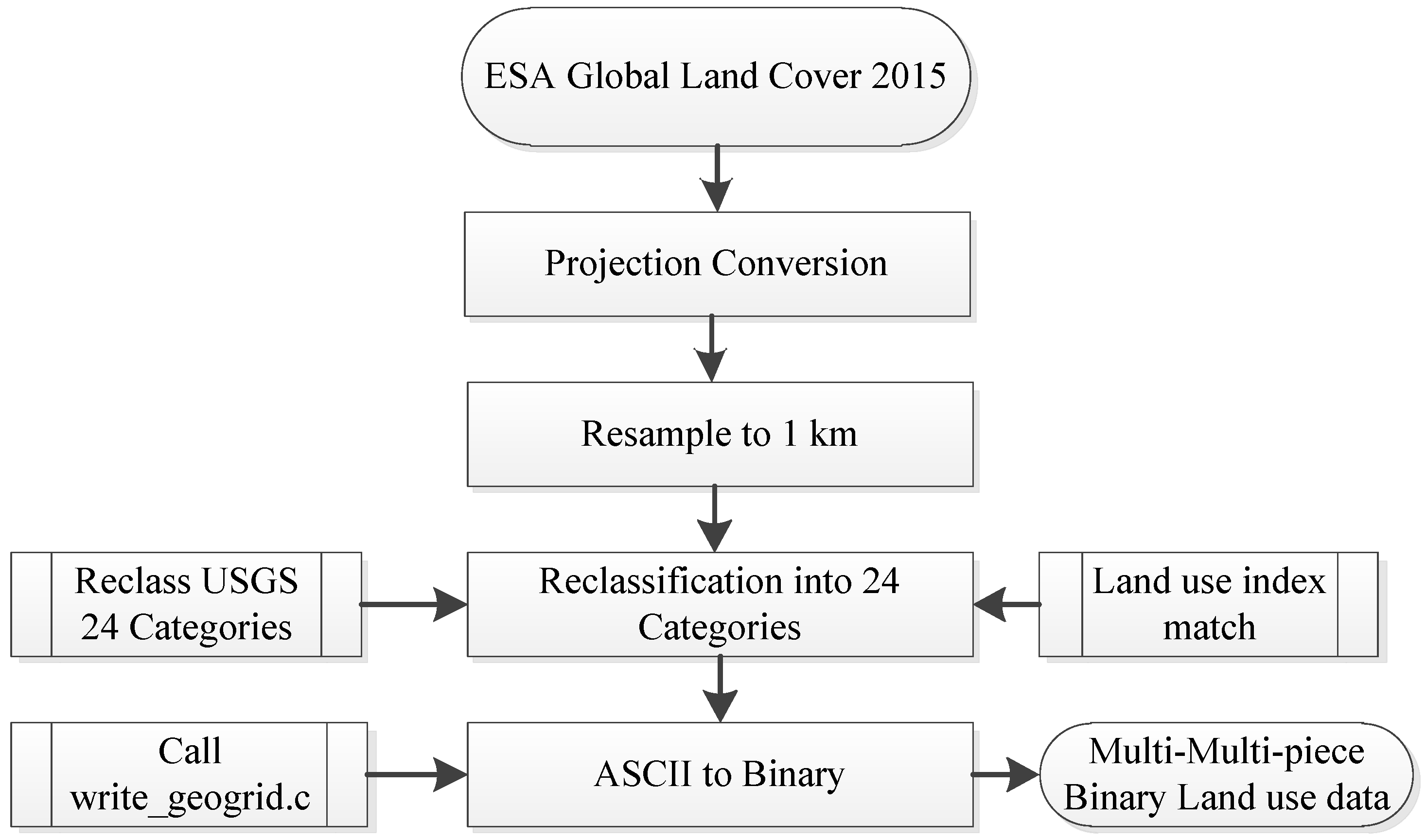
In this study, we generated land-use data based on GLC2015 for the WRF model. The GLC2015 data were up-scaled to a resolution of 1 km and converted into decimal degrees using the GIS (Geographic Information System), because the resolution of WRF’s default land-use data was 30 arcseconds (decimal degree, approximately 1 km). The GLC2015 data were then reclassified to the USGS’s land-use categories according to the classification method of the USGS to ensure the data were consistent with USGS’s classifications, and then they were converted into ASCII format. The similarities among the six physical parameters of each category can be seen in Table 1. The built-in land-use data were divided into 648 binary files, each containing a matrix of size 1200 × 1200 and an index file (metadata). The order of data storage in the matrix was different from that of ordinary remote-sensing data. Moreover, the ASCII data format obtained was incompatible with the WRF Preprocessing System (WPS) module; therefore, format transformation and data decomposition were needed. We established a conversion interface between the GLC2015 data and data from the WRF model, where we used the write_geogrib.c program in the WPS module to convert the internal encoding sequence into a binary format, and wrote the split.c program to divide the data into 648 files and an index file, to ensure the data format was the same as for the USGS data. Figure 1 shows the technical flowchart used to generate the GLC2015 land-use data for use in the WRF model.

Table 1.
Global Land Cover (GLC2015) and United States Geological Survey (USGS) land-use data code conversion table.
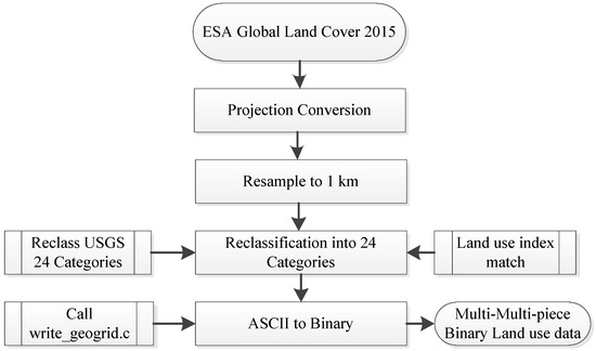
Figure 1.
Technology flowchart.
2.3. Description of the Weather Research and Forecasting (WRF) Model
The WRF-ARW (Advanced Research WRF) Version 3.8.1 model was used in this study. The WRF modeling system has been in development for the past few decades, and is designed to be a flexible, state-of-the-art atmospheric simulation system that is portable and efficient on available parallel computing platforms. The WRF-ARW is suitable for use in a wide range of applications across scales, ranging from meters to thousands of kilometers. WRF is a fully compressible non-hydrostatic model with a horizontal lattice in the Arakawa-C format, and Euler center-based on-terrain following coordinate system. Physical parameterization schemes can be selected in the model, including microphysics, cumulus, planetary boundary layer, and land-surface processes. The WRF model includes the WPS, the WRF model, and the WRF data assimilation (WRFDA) and post-processing systems. The WPS contains the initial data used to define the simulation domain, interpolates terrestrial data (including ground vegetation, terrain, soil type, and land use), and horizontally interpolates the initial data into the simulation domains [25,26].
2.4. Experiment Design
A series of comparative simulations were carried out in Xinjiang from June to August 2018 using WRF3.8.1 (due to the intense land–air interaction in summer and less clouds, because in winter it is mostly covered by snow). The nested domain and topography are shown in Figure 2. The grid spacing was 9 km and 3 km for D01 and D02, respectively. The model was vertically divided into 50 layers and was nested in two domains. Domain1 (D01 hereafter) covered Central Asia and China with 712 × 532 grid points, where the central Asian region was Xinjiang’s upstream weather area as the main source of water vapor transport. Domain2 (D02 hereafter) covered Xinjiang and its western mountainous areas with 832 × 652 grid points. The parameterization schemes of the physical processes were as follows: the microphysics scheme used was the WSM6 (WRF Single Moment 6 class) and cumulus parameterization was the Kain–Fritsch scheme (D02 without cumulus parameterization). RRTMG (Rapid Radiative Transfer Model for GCMs (Global Climate Models)) was selected for both long-wave and short-wave radiation, the planetary boundary layer scheme was ACM2, and the land surface scheme was the NOAH land surface model. Two groups of experiments were designed to test the GLC2015 and USGS datasets. Two sets of geogrid files were created by the WPS as well. Other statistical data and configurations of the input parameters were the same as before. The 0.5° × 0.5° GFS (Global Forecast System) data (http://www.nco.ncep.noaa.gov) from the National Centers for Environmental Prediction (NCEP) were used to provide the boundary and initial conditions, the simulation duration was 24 hours and the output of the D02 domain was hourly. In addition, hourly observations of T2, wind, surface skin temperature (Tsk), relative humidity (RH) and specific humidity (Q2) were collected from 105 automized national meteorological stations in Xinjiang and were used for evaluation.
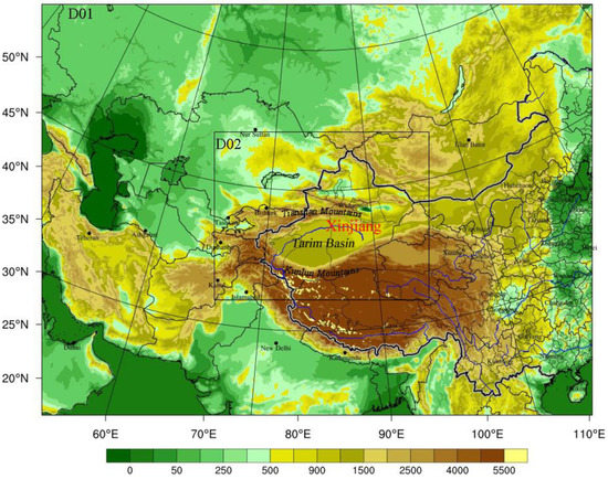
Figure 2.
Two nested domains and topography.
2.5. Assessment Methods
To objectively evaluate the effect of the forecasting simulations, differences in the spatial distributions of the LU_INDEX (Land use Index), and surface energy flux densities between day and night between the simulations using the GLC2015 and USGS land-use data were compared. The root mean square error (RMSE) and Bias of the forecasted T2 and wind against observations from station were used in the analysis as follows:
where Si is the simulated value at i moment of each station, Oi is the observed value at i moment of each station, and N is the sample size.
3. Results and Discussion
3.1. Comparison of the Differences in the Derived Land-Use and Land Parameters
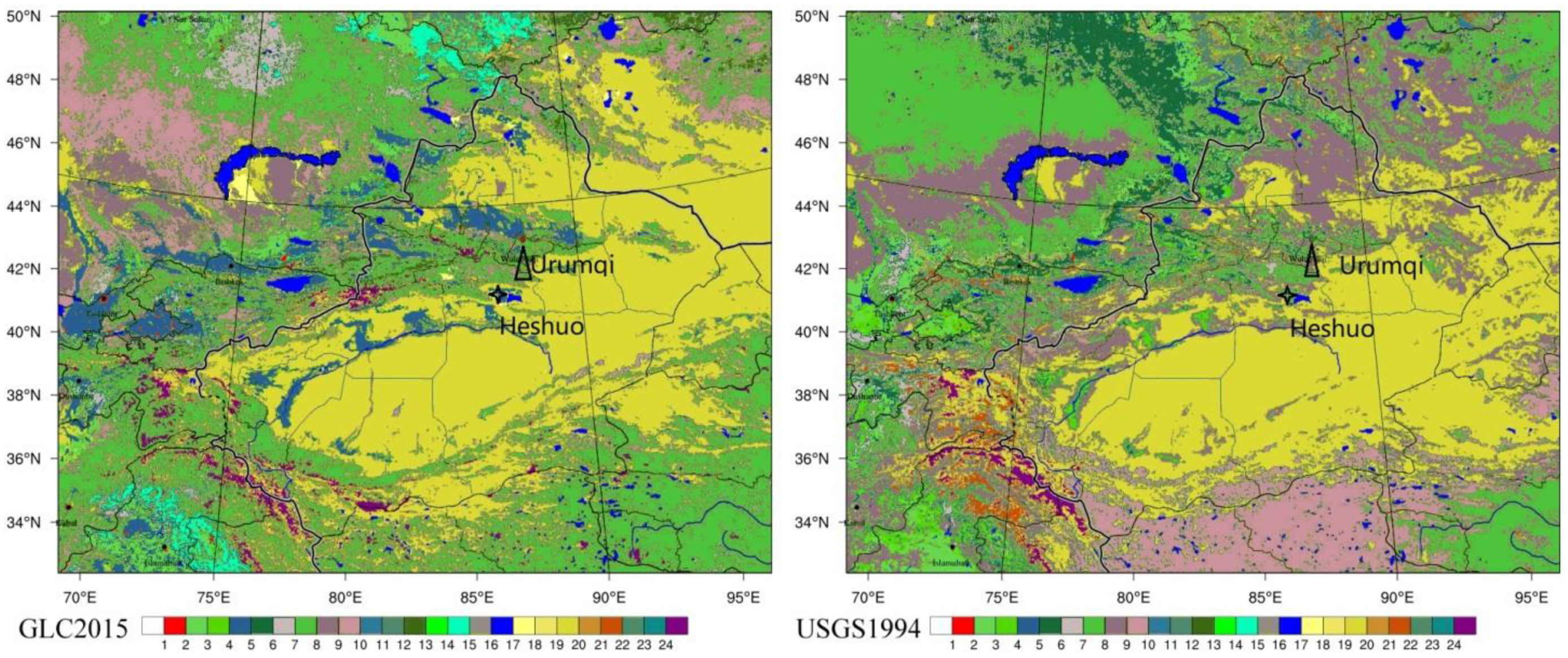
At first, we compared the land-use category distributions and each land-use type percentage of USGS and GLC2015, as shown in Figure 3 and Table 2. Significant differences were seen in their distributions in north Xinjiang and its southern regions. GLC2015 covered 33.11% area of barren or sparsely vegetated surfaces while the USGS only covered 27.6% of the same surface (the land-use types reference to the classification codes Table 1). The total area of urban and built-up land increased obviously in GLC2015, for example, the increase of urbanization in Urumqi was clearly reflected in the GLC2015 data for the past few years; in contrast, urban areas in the USGS covered only 0.083% of the total land area, where there were the distributed sparse grassland (category 7), and sparse vegetation and bare land (category 19), native plants with low vegetative cover fraction. The oasis around the Tarim Basin was seen to have expanded in GLC2015, and 7.2% of the oasis cropland pixels in USGS changed from mixed dryland/irrigated (category 2, 3) to dryland cropland and pasture (category 4); only 5.2% of the area was seen in GLC2015. Shrublands (category 8) reduced by 84% (relative to USGS) and changed into grassland (category 7) in GLC2015, where the most clearly changed areas were distributed in southern Xinjiang and the Tibetan Plateau. The central area of the Tianshan Mountains was generally covered with permanent snow and ice (category 24) in GLC2015, however no snow or ice were detected in USGS even though prominent ice/snow cover on the Tianshan Mountains and Kunlun Mountains could be seen in the online satellite map (https://map.baidu.com). This clearly illustrates that the GLC2015 presents more realistic land-use distributions.

Figure 3.
LU_INDEX (Land use Index) maps of the GLC2015 and USGS land-use data.

Table 2.
Land-use type statistic and percentage changes of GLC2015 and USGS.
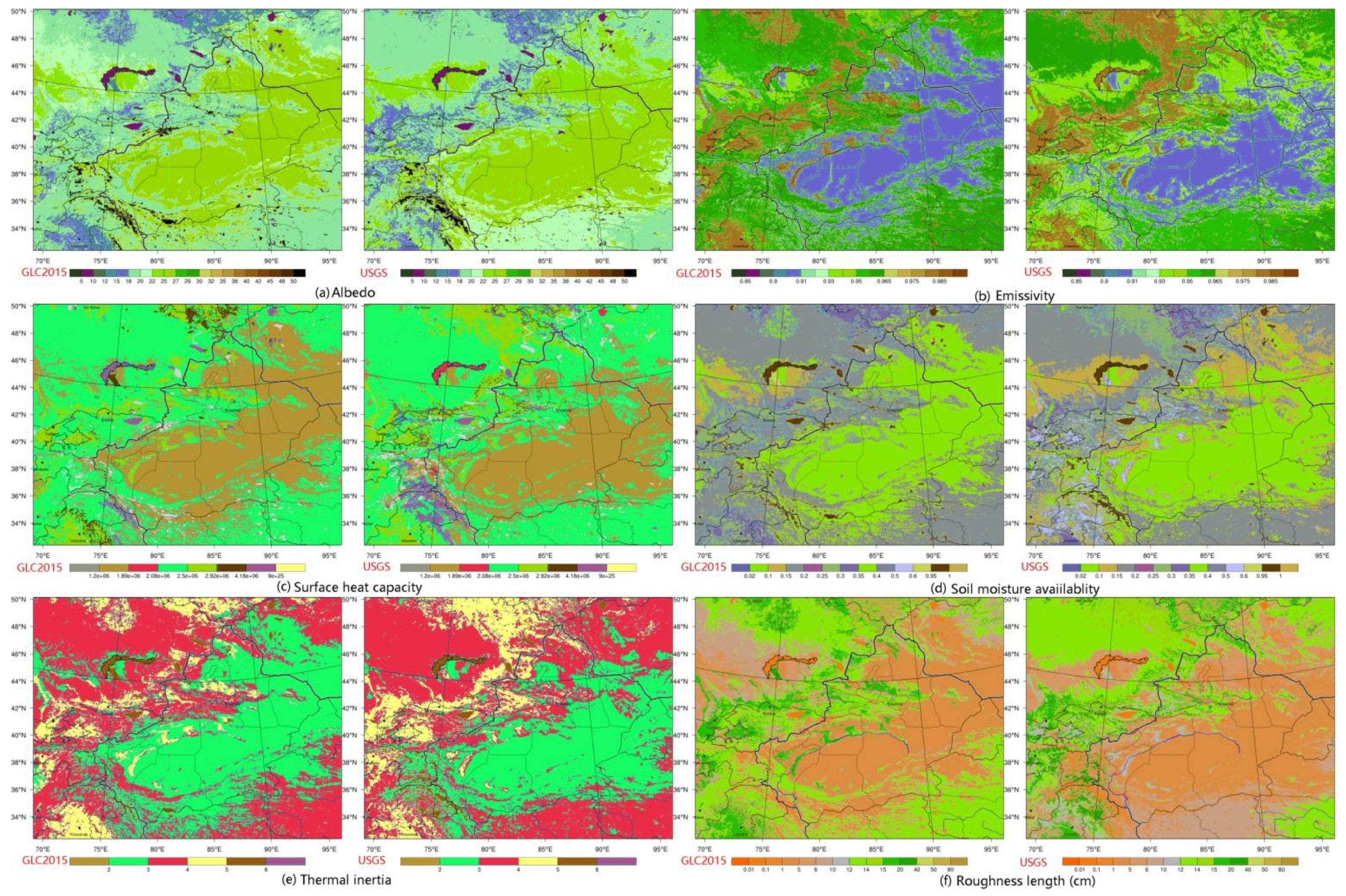
Updated land-use data can directly alter the values of relevant surface parameters, including the surface albedo, emissivity, surface heat capacity, soil moisture availability, thermal inertia and surface roughness. Figure 4 shows maps of six main land parameters derived from the two sets of land-use classification data in D02. Higher albedos (Figure 4a) were seen in northern areas of Xinjiang, which resulted from the land-use type changing from category 7 “Grassland” in USGS to category 19 “Barren or Sparsely Vegetated” in GLC2015. Higher albedos were also seen in the USGS data in areas containing snow and ice on the Tianshan Mountains and Kunlun Mountains. The albedos of oases around the Tarim Basin were also reduced due to a remarkable expansion of crop land. Figure 4b shows that northern regions of Xinjiang have lower emissivity arising from of category-19 areas in GLC2015, and the surface heat capacities (Figure 4c) also differed between GLC2015 and USGS in areas where the land-use types changed significantly, such as in lower distributed areas of northern Xinjiang; soil moisture availability and thermal inertia were also lower in these areas (Figure 4d).

Figure 4.
Spatial distribution of the six main physical land parameters in the GLC2015 and USGS land-use datasets for D02: (a) surface albedo (%), (b) surface emissivity, (c) surface heat capacity, (d) soil moisture availability, (e) thermal inertia, and (f) roughness length (cm).
3.2. Impacts of Land-Use Change on Surface Energy Fluxes
Due to advective processes in the atmosphere, land-use change can potentially influence meteorological processes in the entire domain. Therefore, looking closely at the direct impact of these processes can help us to understand the main mechanisms that lead to changes in near-surface variables. To investigate this, two places where the land use had changed significantly were chosen: the stations at Heshuo and Urumqi. Urumqi is covered with grassland in USGS; however, considerable development has occurred during the past few decades, and due to this urban expansion, urban areas and built-up land is seen in GLC2015. Heshuo is covered with irrigated cropland and pasture in USGS, which consist of planted cotton, industrial pepper, and tomatoes. These crops have been watered using drip and spray irrigation in recent years, and thus the land-use type is mixed dryland irrigated cropland in GLC2015.
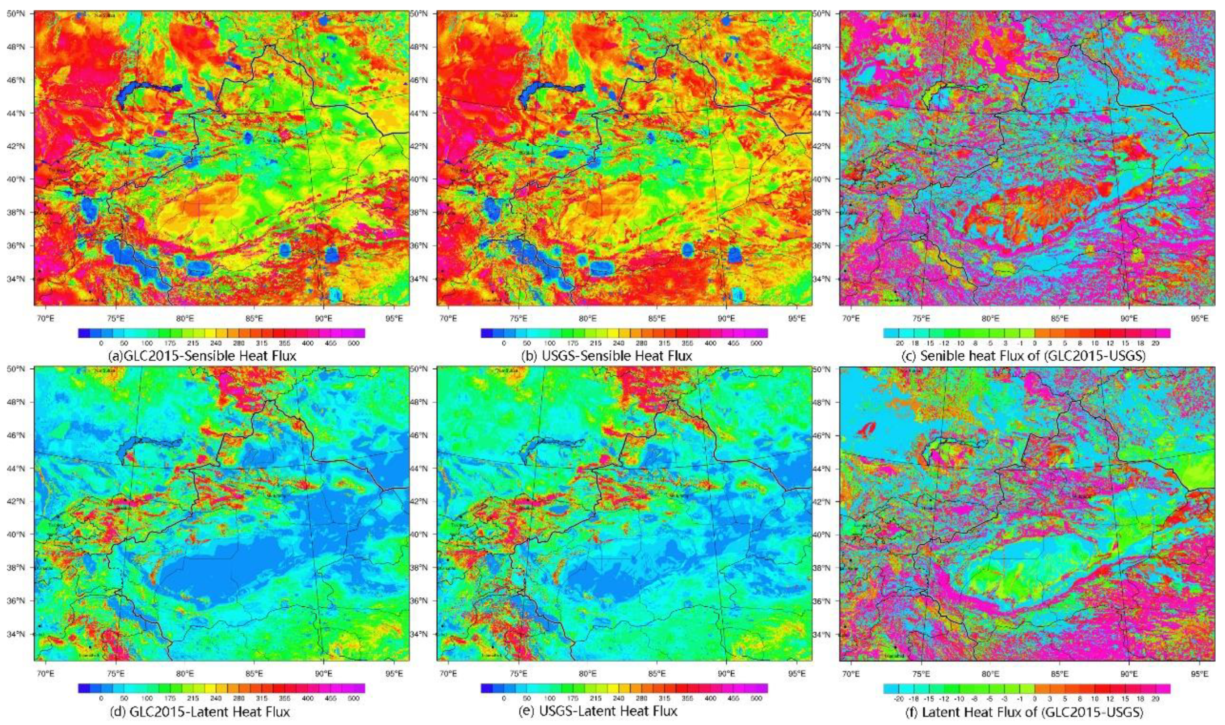
Land surface albedo and emissivity are very sensitive to energy flux arising from the ground, and any change of land use can lead to changes in albedo and emissivity. The albedo determines the absorption of solar shortwave radiation energy by the surface, and emissivity affects the amount of longwave radiation travelling from the surface to the sky. Figure 5 shows the difference in the sensible heat flux (SHF) and latent heat flux (LHF) between the GLC2015 and USGS land-use data at 6:00 UTC summer period (This is generally, the time of the highest temperature in Xinjiang, approximately at a local time of 14:00). Figure 5a shows that the SHF is lower over northern Xinjiang, most likely resulting from the increased albedo and reduced emissivity in this area. Here, a higher albedo results in more solar radiation being reflected back to the sky, and hence less radiation being absorbed by the atmosphere. Furthermore, a lower emissivity will reduce the amount of longwave radiation emitted back to the atmosphere. By comparing the changes in the energy flux, we see that the changes in the surface type affect heat exchange between the surface and the atmosphere, and thus the forecasted temperature:
where H is the sensible heat flux, Rnet is the net radiation, SD and LD are the downward shortwave and longwave radiation, respectively, Tsfc is the surface temperature, σ is the Stefan–Boltzmann constant, α and E are the surface albedo and surface emissivity, respectively, LE is the latent heat flux, and G0 is soil heat flux [27].
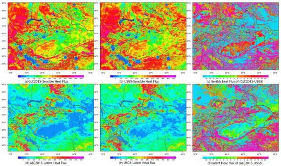
Figure 5.
Contrast maps of the sensible and latent heat fluxes of GLC2015 (a,c) and USGS (b,d) and their differences at 6:00 UTC, 10 July 2018.
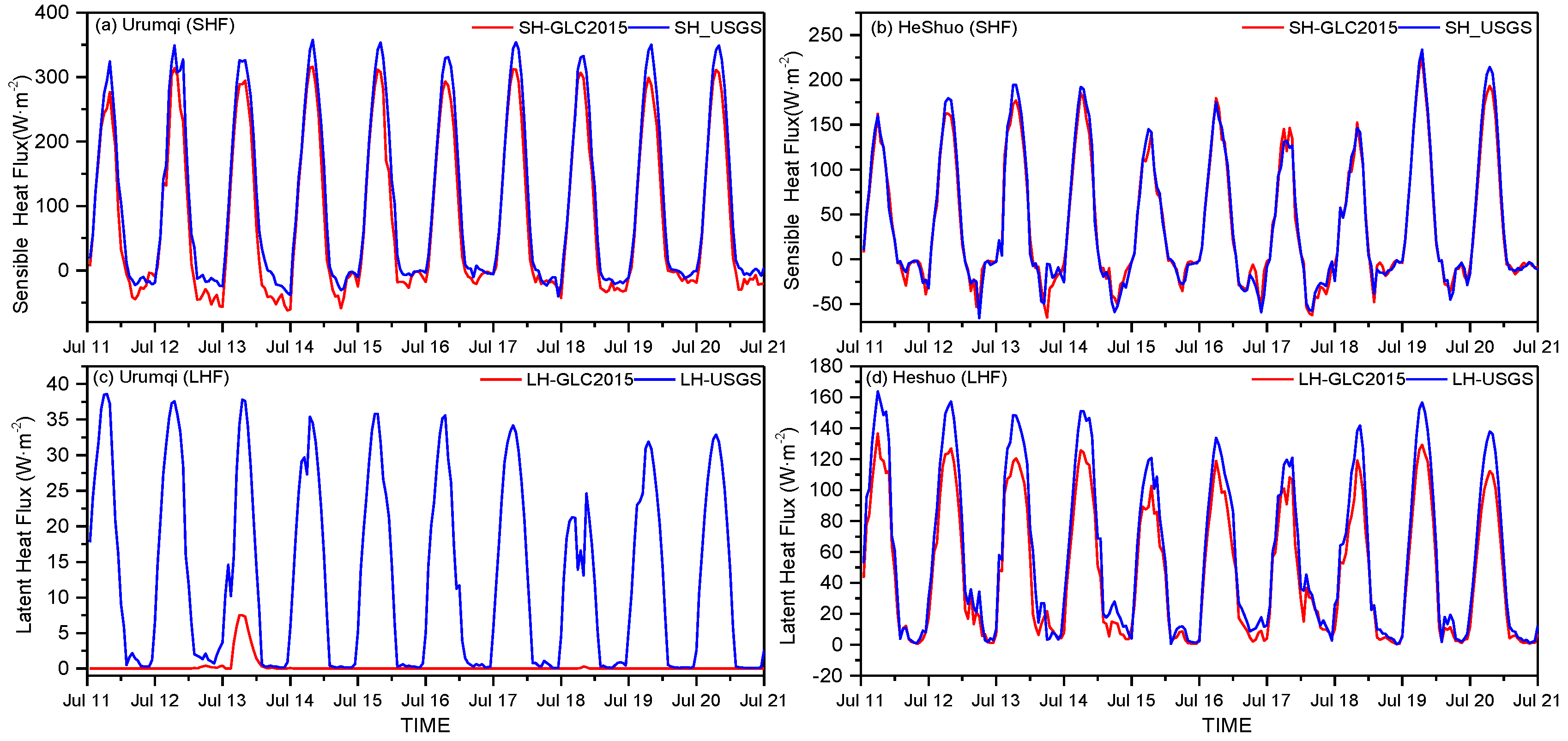
According to Equation (3), for the same amount of radiation, if more shortwave radiation is reflected to the sky the amount of heat stored on the surface will decrease. Sensible heat forms by turbulence after the atmosphere is heated by longwave radiation. Thus, the simulated SHF values in the desert/Gobi regions decreased more than was measured. Additionally, the simulated LHF values also reduced due to the lower soil moisture availability in GLC2015. The SHF values in the Taklimakan Desert observed a small change over 20 W·m−2. From Figure 3a,b, it is clearly illustrated that the edge of the desert in southern Xinjiang was updated to dryland cropland in GLC2015 from irrigated cropland in USGS, which resulted in that an increased albedo and reduced heat storage in the ground; hence, the SHF was reduced by the same mechanism. The vegetation types changed as a consequence of the decreased soil moisture, and the simulated vegetation types accorded more with the observations. The surface evapotranspiration also changed because of the decreased LHF forcing evaporation in oasis regions and the desert in northern Xinjiang. Evapotranspiration in the Gobi regions of eastern Xinjiang decreased significantly after the surface type had been updated to desert/Gobi, and LHF decreased by more than 20 W·m−2 compared with that in the original USGS. From Figure 6a,c, the land use changed to urban areas from grassland in Urumqi, in which the SHF in GLC2015 reduced obviously at noon, and LHF declined sharply to nearly zero; the cause of these changes was that the urban surface had little evaporation capacity during sunny days. Figure 6b,d show comparisons of SHF and LHF between GLC2015 and USGS. Small differences are seen in the simulated SHF values, but the LHF values decreased more at noon in GLC2015 compared to USGS. Indeed, as dryland crops imply lower soil moisture availability, and hence less soil moisture is maintained in the group, evaporation reduced, and hence the SHF reduced accordingly.
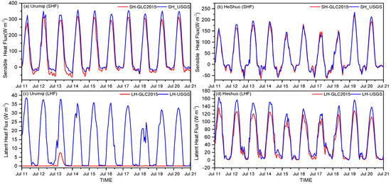
Figure 6.
Sensible heat flux (SHF) at (a) Urumqi and (b) Heshuo, and the latent heat flux (LH) at (c) Urumqi and (d) Heshuo (d). Both GLC2015 (red line) and USGS (blue line) are plotted.
3.3. Impacts of Land-Use Change on the Air Temperature and Surface Skin Temperature
The updated land-use data changed the derived surface parameters, whose variations further induced changes in the amount of radiation that was absorbed or reflected; these consequently changed the surface skin temperature and air temperature. Surface skin temperature and air temperature are affected by the downward radiation flux, surface albedo, emissivity, and soil water content. Albedo determines the amount of solar radiation absorbed by the surface, where the surface absorbs solar shortwave radiation and transfers it to the soil, which increases the surface temperature and leads to heat being stored in the sub-layer soil during the daytime. The emissivity determines the amount of radiation that goes to heating the air [28]. On sunny days land-surface processes play a more prominent role in the WRF model. In order to detect any obvious differences in the model when using the updated land-use data, we chose to model the high-temperature weather processes on a sunny day in the summer. The air was heated by upward longwave radiation and convective from the ground, where Equation (4) expresses the method used to calculate the surface temperature. Emissivity is a key parameter that determines the amount of surface-to-air radiation, which in turn affects changes in both daytime and nighttime temperatures:
where and are the downward and upward longwave radiation, respectively. In the WRF model, T2m is diagnosed by means of:
where ρ and cp are the air density and heat capacity of the air, respectively, κ=0.4 is the von Karman’s constant, z0h is the roughness length for heat, ψH is the integrated universal function for heat, and u* represents the friction velocity at 2 m.
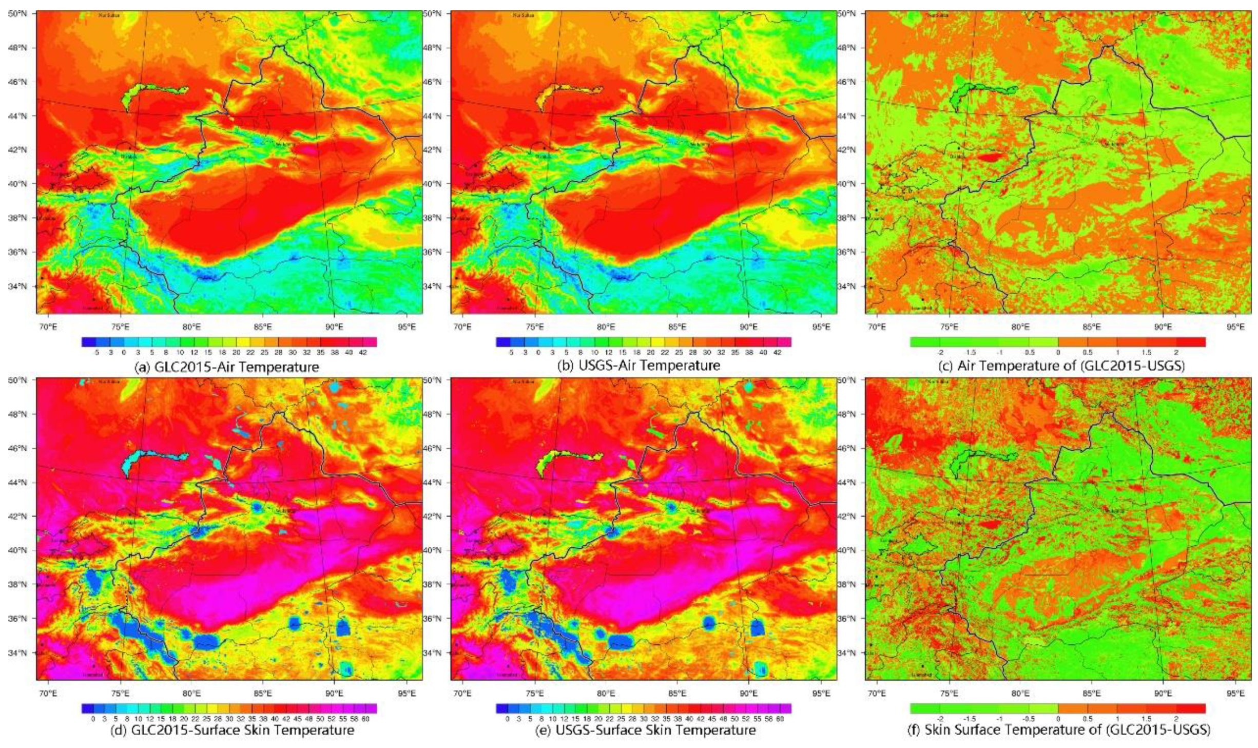
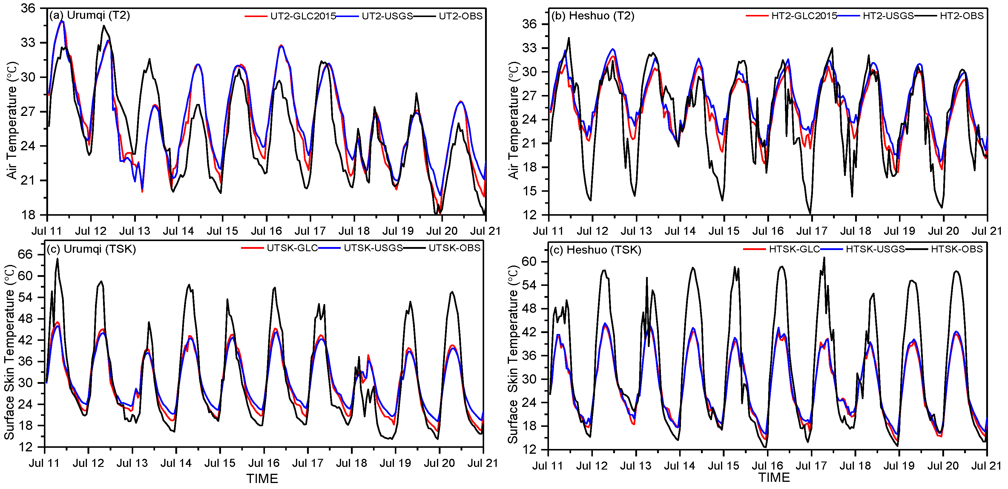
Figure 7 compares the air temperature and skin surface temperature in D02 found using GLC2015 (Figure 7a,d and USGS (Figure 7b,e). Their differences at 6:00 UTC (the maximum temperature period) on 11 July 2018 are shown in Figure 7c,f, where it can be seen that the maximum air and surface skin temperatures in GLC2015 were lower than those in USGS for northern Xinjiang and oasis croplands in southern Xinjiang. Figure 8 also shows the air temperature and surface skin temperature and their observed variations at the Urumqi and Heshuo stations. Figure 8a,c indicate that the daily maximum air temperature of Urumqi was approximately the same between GLC2015 and USGS. However, the surface skin temperature in GLC2015 was slightly higher than in USGS, and the nocturnal minimum temperature in GLC2015 was significantly lower than in USGS. The reason for these differences may be that the thermal inertia and surface heat capacity in cities are lower than in grasslands; thus heat preservation on the surface of a city is lower than that of grassland, which explains why the surface skin temperature of GLC2015 is lower than that of USGS. Indeed, the former is much closer to the observations, which indicates that more realistic parameters can lead to improved temperature forecasts due to a better representation of land use. At Heshuo station (Figure 8b,d), the minimum air temperature was significantly underestimated by both GLC2015 and USGS. Although the latter dataset was closer to observations, where land use changed from irrigated croplands to mixed dryland irrigated croplands, which meant the soil moisture availability was reduced by half, which led predominantly to the decreased nighttime air temperature.
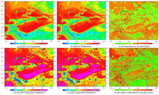
Figure 7.
Contrast maps of air temperature and skin surface temperature of GLC2015 (a,c) and USGS (b,d) and their differences at 6:00 UTC, 11 July 2018.
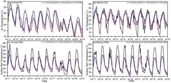
Figure 8.
Air temperature (T2) at (a) Urumqi and (b) Heshuo, and the surface skin temperature (TSK) at (c) Urumqi and (d) Heshuo. Both GLC2015 (red line) and USGS (blue line) are shown.
3.4. Impacts of Land-Use Change on the Wind Speed
The simulated wind speeds of the WRF model were divided into zonal (U wind) and meridional (V wind) velocity components. The influence of land-use changes on the wind field is complex and uncertain in some places. The wind speeds were determined diagnostically by means of the Monin–Obukhov similarity theory under the assumption of atmospheric stability. In addition to deviations in the background field, a main factor influencing the near-surface layer is the surface roughness, while the roughness length (z0m) is the key parameter influencing the wind speed. The wind speed can be calculated as follows:
In Equation (7), U(z) is the horizontal wind velocity at height z above the ground, u* is the frictional velocity, and κ is the von Kalman constant, which has a value of 0.4 in this work [25].
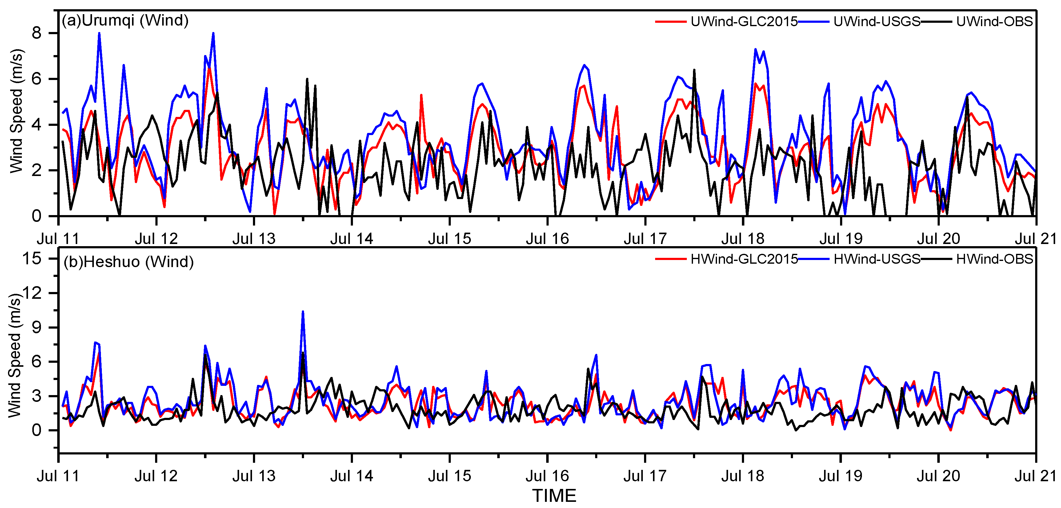
The effect of surface roughness on the wind speed was calculated using Equation (7) [29]. Figure 9a compares the simulated surface wind speeds with observations at Urumqi station. It was seen that the simulated wind speeds did not agree well with the observations, where the differences between GLC2015 and USGS reached 2 m/s, and the peak wind speed of GLC2015 was lower than that found using USGS. Our analysis indicated that with the updated land-use data (GLC2015), the underlying surface was replaced with impervious structures such as buildings and city-forest belts, which increased the surface roughness in Urumqi, and reduced the wind speed to some extent. Figure 9b shows a comparison between the observed and simulated surface data at Heshuo station, where the land is covered by irrigated cropland and pasture in USGS, but the renewed land use is mixed dryland irrigated cropland in GLC2015. Thereby, z0m increased from 0.1 m to 0.15 m, and the USGS simulated values were in better agreement with the observations.
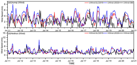
Figure 9.
Simulated and observed wind speeds at (a) Urumqi and (b) Heshuo. GLC2015 (red line), USGS (blue line) and observational (black line) data are shown.
3.5. Impacts of Land-Use Change on the Specific Humidity and Relative Humidity
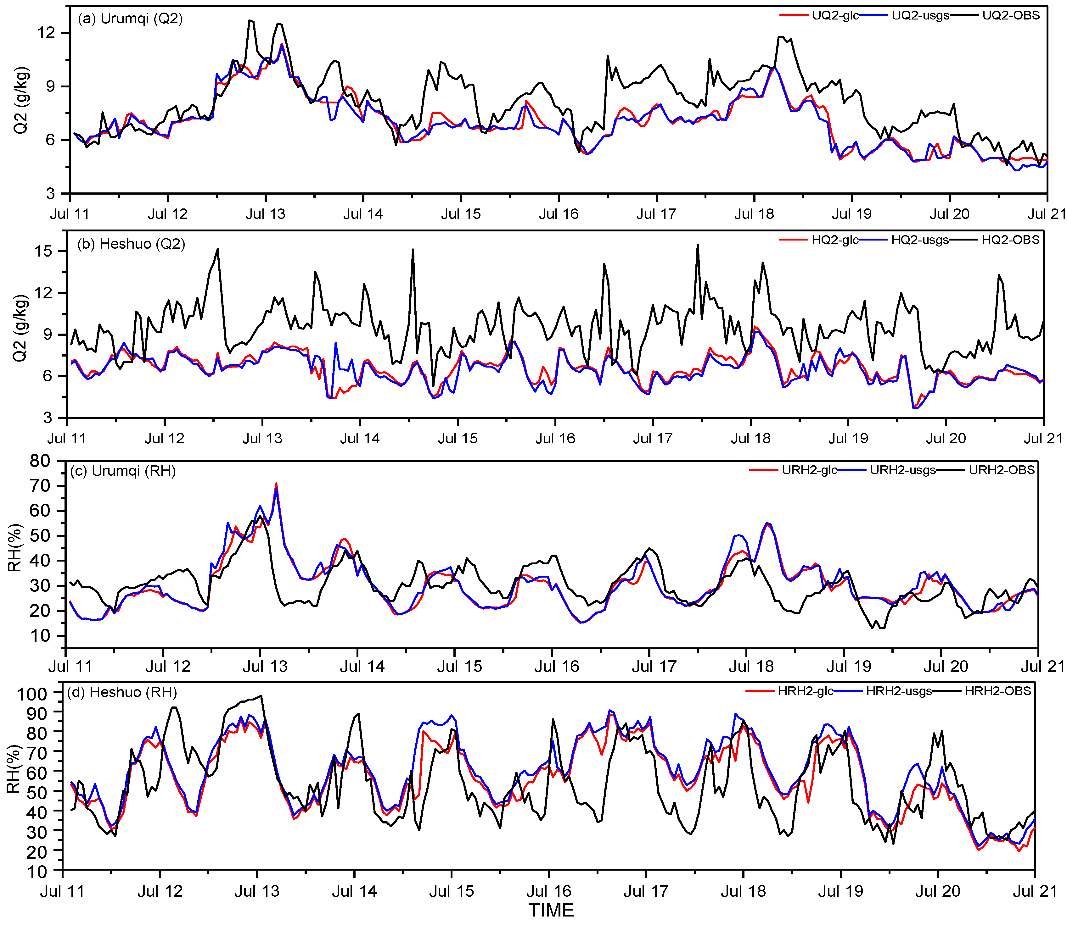
The specific humidity at 2 m is directly related to air and surface temperature, soil moisture and rainfall, where cold temperatures produce less water vapor than warm air from soil and/or vegetation. Although the effect of the new dataset on temperature forecast indicates improvement, Figure 10a shows a comparison of the simulated and observed specific humidity at Urumqi. There was no clear difference between corresponding GLC2015 and USGS fields, where both showed similar trends with the observed data. For long periods Urumqi received no rain, which formed a xerothermic environment; consequently there was insufficient water for significant levels of evapotranspiration. As a result, the specific humidity was below 10 g/kg after 13 July, the diurnal variation of specific humidity without clearly peak value, and the specific humidity values predicted by both simulations were less than observations. Figure 10b illustrates the specific humidity diurnal variations between the simulations and observations at Heshuo station during the period. Both simulations underestimated the specific humidity significantly, there was no clear difference between GLC2015 and USGS, and they were without similar variations in the tendency to the observations. Figure 10c shows a comparison of the simulated and measured relative humidity at Urumqi, where both had similar variation patterns, and there was very little difference between those from GLC2015 and USGS. This result suggests that the WRF model do not have a widespread systematic bias even though the relative humidity is complex and depends on multiple parameters. The simulated relative humidity from GLC2015 was lower than from USGS at some of the peak values and were closer to the observations. This may be because the simulated air temperatures and surface skin temperatures of GLC2015 are lower than those from USGS, where cold air reduces evapotranspiration from ground and vegetation. Figure 10d illustrates the variations of the relative humidity simulated using GLC2015, USGS and the observations. The simulated values were all overestimated during the daytime, although those from GLC2015 were in slightly better agreement with the observed data. Where there in GLC2015 is covered dryland cropland, which represented actual conditions correctly, lower soil moisture availability can hold less water content in soil, so it will result in lower relative humidity.
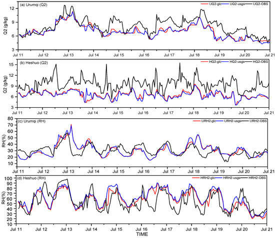
Figure 10.
Q2 and RH at Urumqi (a,c) and Heshuo (b,d). GLC2015 (red line), USGS (blue line) and observations (black line) are shown.
In summary, according to the verifications performed using the observations made by the MET and the 105 national stations, we used the bias and RMSE statistics to compare the air temperature, surface skin temperature, wind speed, specific humidity and relative humidity simulated by GLC2015 and USGS, in order to find any improvements arising from using the updated GLC2015 land-use dataset in D02. From Table 3 we can see that the bias and RMSE of T2 were reduced by 2.54% and 1.48%, respectively, when using the updated GLC2015, which benefited from energy fluxes that were better estimated. Tsk was significantly underestimated during daytime, especially at peak value, but GLC2015 only provided slightly improved nighttime values, as reflected by the bias and RMSE of Tsk being reduced by only 2.48% and 1.98%, respectively, relative to the USGS. The forecasted wind speeds were obviously improved: The bias and RMSE of Winds reduced by 10.48% and 6.77%, respectively. This improvement was mostly attributed to GLC2015 providing a better representation of more actual underlying surface properties, such as the specified value of z0m, which was obtained from a lookup land-use table. The Q2 variations patterns were underestimated and showed a negative bias, although there was almost no bias and RMSE between GLC2015 and USGS. As for RH, which is highly dependent on the temperature, the bias and RMSE of the values found via GLC2015 reduced by 1.87% and 1.05%, respectively, relative to the USGS-predicted values.

Table 3.
Bias and RMSE of the air temperature, surface skin temperature, winds speed, specific humidity and relative humidity simulated by GLC2015 and USGS.
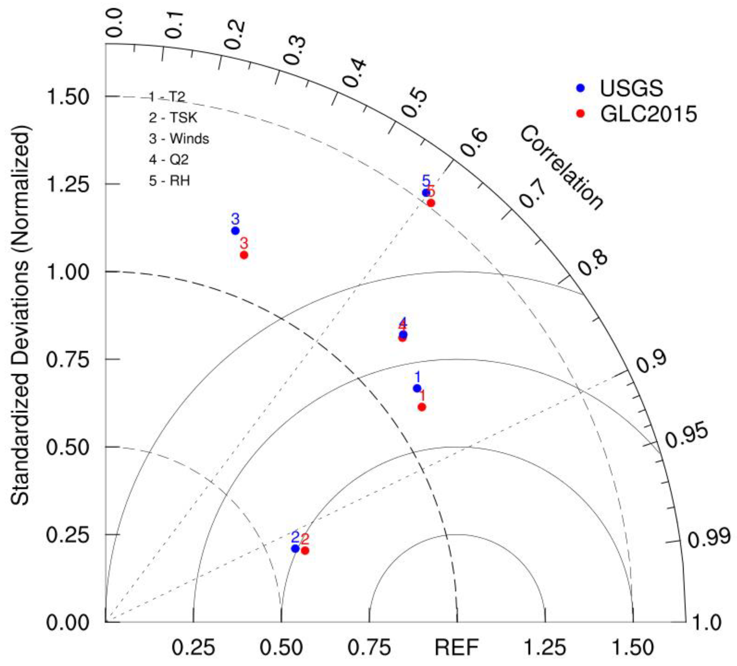
Figure 11 shows a Taylor diagram that compares the performance of the simulations (in terms of the simulated values of T2, Tsk, Winds, Q2 and RH) of GLC2015 and USGS. A Taylor diagram is a graphical method used to comprehensively evaluate the accuracy of models (Taylor, 2001) based on the CC (correlation coefficient), centered RMSE and SD (standard deviation) statistics. The closer a simulated point was to the REF (Reference) point, the better the accuracy of the simulation. Figure 11 illustrates that all but point 4 (red and blue) were close to REF. The Winds simulations had poor correlations, but red point 3 was closer to the REF value relative to blue point 3, which indicated that the Winds values found using GLC2015 had better correlation and lower RMSE than those from USGS. For Q2, the blue and red points (both labelled as 4) nearly overlap, which indicated that Q2 showed basically no improvement with the new dataset. The general conclusion from the above statistical evaluations of the simulations after using the updated GLC2015 land-use data, was that the simulation performance of the WRF model generally improved as a whole, but that these improvements were modest.
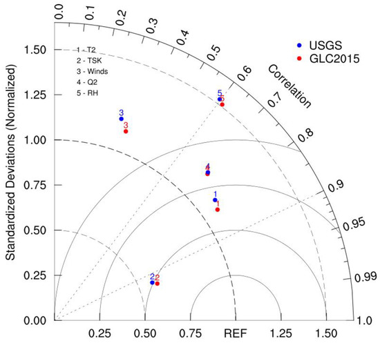
Figure 11.
Taylor diagram of the performance of T2, Tsk, Winds, Q2 and RH simulated using the GLC2015 and USGS data for whole D02 domain (red points indicate GLC2015 values, and blue are USGS values).
4. Conclusions
In this study, we developed a new land-use dataset based on GLC2015 remote-sensing products to be used in the WRF model. It was seen that the updated data better represented land-use characteristics that have changed in recent years, due to changes to both land-use and climate. Compared with the default USGS data currently utilized in the WRF model, in terms of the LU_INDEX generated by the WRF model via the two sets of land-use data, the GLC2015 data more accurately represented the actual underlying surface of the Xinjiang region. This new dataset also properly reflected the process of urbanization in Urumqi, correctly illustrated the oasis expansion around the Tarim Basin in southern Xinjiang, and correctly displayed ice/snow cover on the Tianshan Mountains, in accordance with observations. In addition, we analyzed changes of land surface parameters caused by updates in land-use specification.
Based on the two sets of land-use data, we designed two group experiments (GLC2015 vs. USGS) to evaluate their impacts on the simulated values of near-surface atmospheric variables (T2, Tsk, Winds, Q2 and RH) compared with observations. The surface energy fluxes (SHF, LH) were also contrasted. In our comparison we chose two typical stations (Urumqi, Heshuo) where the land use had changed dramatically in recent times, and we analyzed the mechanisms underlying the differences in the near-surface atmospheric variables and air-land flux changes due to the land-use changes. Afterwards, we used observational data obtained by the MET and 105 national stations to verify the simulations using the bias and RMSE statistics in the D02 domain. Finally, we produced a Taylor diagram to comprehensively evaluate the performance of each simulation.
The land-use category changes modified the corresponding land surface parameters, which in turn affected the modelled land-air interactions and thus impacted the derived surface energy fluxes. The impact of the changed land-use types on the simulated SFH and LH values were contrasted at the Urumqi and Heshuo stations. It was shown that SFH was sensitive to albedo and emissivity, and LH was sensitive to soil moisture availability, over northern Xinjiang, whereby SFH and LH decreased obviously where the grassland changed into desert. It was also found that Tsk was closely related to energy fluxes, furthermore explaining the reason for how T2 was influenced, thermal convection from surface heat exchange and long wave radiation, so it is sensitive to emissivity and z0m. Furthermore, it was shown that RH mainly depended on T2, where a lower maximum T2 during the daytime produced less water vapor in the air. The parameter Winds is determined by means of Monin–Obukhov similarity theory, in which z0m was a very important parameter, the actual z0m reduced the overestimation of wind speed.
The bias and RMSE values, as well as the Taylor diagram, illustrated that the simulated near surface variables (expect for Q2) improved when using the updated GLC2015 land-use data. This demonstrated that the GLC2015 land-use data had better representation of actual conditions, and hence improved forecast capability. Generally, forecasts of near-surface variables are influenced by different synoptic conditions during each season; thus, long time scales are needed to verify the performance of the new dataset in different seasons, and hence determine whether GLC2015 can effectively improve numerical weather forecasting for the entire year. In general, the application of the new GLC2015 land-use dataset is expected to improve numerical weather simulations and enhance weather forecasting capability in the Xinjiang area.
Author Contributions
For research articles with several authors, a short paragraph specifying their individual contributions must be provided. The following statements should be used “Conceptualization, H.L. and H.Z.; methodology, S.F.; software, H.L.; validation, C.J., and H.Z.; formal analysis, H.L.; investigation, H.L.; resources, A.M.; data curation, C.J.; writing—original draft preparation, H.L.; writing—review and editing, S.F.; visualization, H.L.; supervision, Z.L.; project administration, S.F.; funding acquisition, A.M. All authors have read and agreed to the published version of the manuscript.
Funding
The research was supported by the National Key Research and Development Program of China (2018YFC1507105), and the National Natural Science Foundation of China (41801019, 41875023), the Research Foundation of Central Asian for Atmospheric Science (CAAS201811).
Acknowledgments
Thanks to Junjian Liu provided GFS data and program to process GLC2015 data.
Conflicts of Interest
The authors declare no conflict of interest.
References
- Chen, F.; Zhang, Y. On the coupling strength between the land surface and the atmosphere: From viewpoint of surface exchange coefficients. Geophys. Res. Lett. 2009, 36, 207–213. [Google Scholar] [CrossRef]
- Mahmood, R.; Pielke, R.; Mcalpine, C.A. Climate-relevant land use and land cover change policies. Bull. Amer. Meteorol. Soc. 2016, 97, 195–202. [Google Scholar] [CrossRef]
- Jiménez-Esteve, B.; Udina, M.; Soler, M.R.; Pepin, N.; Miró, J.R. Land use and topography influence in a complex terrain area: A high resolution mesoscale modelling study over the Eastern Pyrenees using the WRF Model. Atmos. Res. 2017, 202, 49–62. [Google Scholar] [CrossRef]
- Hong, S.; Lakshmi, V.; Small, E.; Chen, F.; Tewari, M.; Manning, K.W. Effects of vegetation and soil moisture on the simulated land surface processes from the coupled WRF/Noah model. J. Geophys. Res. Atmos. 2009, 114, 1211–1225. [Google Scholar] [CrossRef]
- Gilliam, R.C.; Pleim, J.E. Performance assessment of new land surface and planetary boundary layer physics in the WRF-ARW. J. Appl. Meteorol. Clim. 2008, 49, 760–774. [Google Scholar] [CrossRef]
- Cheng, F.Y.; Hsu, Y.C.; Lin, P.L.; Lin, T.H. Investigation of the effects of different land use and land cover patterns on mesoscale meteorological simulations in the Taiwan area. J. Appl. Meteorol. Clim. 2013, 52, 570–587. [Google Scholar] [CrossRef]
- Jiang, X.; Wiedinmyer, C.; Chen, F.; Yang, Z.L.; Lo, J.C.F. Predicted impacts of climate and land use change on surface ozone in the Houston, Texas, area. J. Geophys. Res. Atmos. 2008, 113, D20312. [Google Scholar] [CrossRef]
- Grossman-Clarke, S.; Zehnder, J.A.; Loridan, T.; Grimmond, C.S.B. Contribution of land use changes to near-surface air temperatures during recent summer extreme heat events in the Phoenix metropolitan area. J. Appl. Meteorol. Climatol. 2010, 49, 1649–1664. [Google Scholar] [CrossRef]
- Nguyen, L.H.; Joshi, D.R.; Clay, D.E.; Henebry, G.M. Characterizing land cover/land use from multiple years of Landsat and MODIS time series: A novel approach using land surface phenology modeling and random forest classify. Remote Sens. Environ. 2020, 238, 111017. [Google Scholar] [CrossRef]
- Schicker, I.; Arias, D.A.; Seibert, P. Influences of updated land-use datasets on WRF simulations for two Austrian regions. Meteorol. Atmos. Phys. 2015, 128, 1–23. [Google Scholar] [CrossRef]
- Xuejie, G.; Yong, L.; Wantao, L.; Zongci, Z.; Giorgi, F. Simulation of effects of land use change on climate in China by a regional climate model. Adv. Atmos. Sci. 2003, 20, 583–592. [Google Scholar] [CrossRef]
- Sequera, P.; González, J.E.; McDonald, K.; LaDochy, S.; Comarazamy, D. Improvements in land-use classification for estimating daytime surface temperatures and Sea-Breeze flows in southern California. Earth Interact. 2016, 20, 1–32. [Google Scholar] [CrossRef]
- Santos-Alamillos, F.J.; Pozo-Vázquez, D.; Ruiz-Arias, J.A.; Tovar-Pescador, J. Influence of land-use misrepresentation on the accuracy of WRF wind estimates: Evaluation of GLCC and CORINE land-use maps in southern Spain. Atmos. Res. 2015, 157, 17–28. [Google Scholar] [CrossRef]
- Sertel, E.; Robock, A.; Ormeci, C. Impacts of land cover data quality on regional climate simulations. Int. J. Climatol. 2010, 30, 1942–1953. [Google Scholar] [CrossRef]
- Taha, H. Modeling impacts of increased urban vegetation on ozone air quality in the South Coast Air Basin. Atmos. Environ. 1996, 30, 3423–3430. [Google Scholar] [CrossRef]
- Gao, Y.; Chen, F.; Barlage, M.; Liu, W.; Cheng, G.; Li, X.; Ma, M. Enhancement of land surface information and its impact on atmospheric modeling in the Heihe River Basin, northwest China. J. Geophys. Res. Atmos. 2008, 113, 2739–2740. [Google Scholar] [CrossRef]
- Qu, R.; Cui, X.; Yan, H.; Ma, E.; Zhan, J. Impacts of Land Cover Change on the Near-Surface Temperature in the North China Plain. Adv. Meteorol. 2013, 2013, 409302. [Google Scholar] [CrossRef]
- De Nobletducoudr, N.; Boisier, J.P.; Pitman, A.; Bonan, G.B.; Brovkin, V.; Cruz, F.; Van Der Molen, M.K. Determining robust impacts of land-use-induced land cover changes on surface climate over North America and Eurasia: Results from the first set of LUCID experiments. J. Clim. 2012, 25, 3261–3281. [Google Scholar] [CrossRef]
- Chang, M.; Fan, S.; Wang, X.M. Impact of refined land-cover data on WRF performance over the Pearl River Delta region, China. Acta Sci. Circums. 2014, 34, 1922–1933. [Google Scholar]
- Meij, A.D.; Vinuesa, J. Impact of SRTM and Corine Land Cover data on meteorological parameters using WRF. Atmos. Res. 2014, 143, 351–370. [Google Scholar] [CrossRef]
- Li, Y.; Zhao, C.; Zhang, T.; Wang, W.; Duan, H.; Liu, Y.; Pu, Z. Impacts of land-use data on the simulation of surface air temperature in Northwest China. J. Meteor. Res. 2018, 32, 896–908. [Google Scholar] [CrossRef]
- Abliz, A.; Yang, Y.; Mamat, Z.; Luo, J.; Abdulslam, D.; Xu, Z.; Halik, W. Land-use change and its effects in Charchan Oasis, Xinjiang, China. Land Degrad. Dev. 2016, 28, 106–115. [Google Scholar] [CrossRef]
- Arino, O.; Bicheron, P.; Achard, F.; Latham, J.; Witt, R.; Weber, J.L. Global Cover: The most detailed portrait of Earth. ESA Bull. 2008, 136, 24–31. [Google Scholar]
- Plummer, S.; Lecomte, P.; Doherty, M. The ESA climate change initiative (CCI): A European contribution to the generation of the global climate observing system. Remote Sens. Environ. 2017, 203, 2–8. [Google Scholar] [CrossRef]
- Zoltan, T. Ensemble Forecasting in WRF. Bull. Am. Meteorol. Soc. 2001, 82, 695–698. [Google Scholar]
- Skamarock, W.C.; Klemp, J.B. A time-split nonhydrostatic atmospheric model for weather research and forecasting applications. J. Comput. Phys. 2008, 227, 3465–3485. [Google Scholar] [CrossRef]
- Chen, Y.; Yang, K.; He, J.; Qin, J.; Shi, J.; Du, J.; He, Q. Improving land surface temperature modeling for dry land of China. J. Geophys. Res. Atmos. 2011, 116, D20104. [Google Scholar] [CrossRef]
- Sun, J.; Mahrt, L. Relationship of surface heat flux to microscale temperature variations: Application to boreas. Bound. Layer Meteor. 1995, 76, 291–301. [Google Scholar] [CrossRef][Green Version]
- Kondo, J.; Yamazawa, H. Aerodynamic roughness over an inhomogeneous ground surface. Bound. Layer Meteor. 1986, 35, 331–348. [Google Scholar] [CrossRef]
© 2020 by the authors. Licensee MDPI, Basel, Switzerland. This article is an open access article distributed under the terms and conditions of the Creative Commons Attribution (CC BY) license (http://creativecommons.org/licenses/by/4.0/).

