Damaging Convective and Non-Convective Winds in Southwestern Iberia during Windstorm Xola

Abstract

On 23/12/2009, windstorm Xola struck mainland Portugal, causing serious damage in a small area north of Lisbon (Oeste region) and in the south region, inflicting economic losses of over EUR 100 million. In both areas, several power towers, designed to withstand up to 46 m s⁻¹ winds, were destroyed. The causes of these two distinct damaging wind events were investigated. Xola was revealed to have a prominent cloud head and a split cold front structure. In the southern region, the damages were due to downburst winds, associated with a mesovortex, observed in a bow echo line triggered by an upper cold front. The cloud head presented several dry air intrusion signatures, co-located with tops progressively lowering towards the hooked tip. This tip revealed features consistent with the presence of slantwise convection, the descending branches of which may have been strengthened by evaporating cooling. At the reflectivity cloud head tip, a jet streak pattern was identified on weather radar, with Doppler velocities exceeding 55 m s⁻¹, just 400 m above ground. This signature is coherent with the presence of a Sting jet, and this phenomenon was associated with the strongest wind gusts (over 40 m s⁻¹) and the largest damages in the Oeste region.

1. Introduction

Extratropical cyclones, and in particular rapidly deepening extratropical cyclones, are known to cause damaging winds. Therefore, over the decades, conceptual models have been developed to help forecasters identify precursors of hazardous weather associated with such storms. Shapiro and Keyser [1] proposed a new conceptual life-cycle model of extratropical cyclones, associated with damaging winds, characterized by four stages: (I) incipient frontal cyclone; (II) frontal fracture, when the cold front loses contact with the warm front, (III) frontal T-bone (cold and warm fronts nearly perpendicular) and bent-back front; and (IV) warm core seclusion (Figure S1). The extensive cloud wrapping around the poleward side of the cyclone core is described as the cloud head (Browning [2], their Figure 4) and it becomes well defined at stage III of the Shapiro–Keyser (S-K) model [3]. At stage IV, the cold air in the dry slot encircles the cyclone center, leading to the seclusion of warm air surrounded by the tail of the bent-back front and the associated tip of the cloud head [3]. The dry slot is a cloud-free zone, indicative of the dry intrusion approaching the center of a developing cyclone [2,4]. Dry intrusion is an air stream that descends from the upper troposphere and lower stratosphere into the middle and low tropospheric levels [4]. Therefore, due to its low moisture content, dry intrusion can be identified in water vapor (WV) channel satellite imageries as a dark zone [2]. The cloud head and the dry slot are characteristic features of cyclones that cause damaging winds [3].

Hewson and Neu [5] analyzed the characteristics of 29 historic windstorms that affected the North Atlantic and Europe, and categorized them according to the presence of three windstorm phenomena: the warm jet (WJ), the cold jet (CJ) and the sting jet (SJ). Out of these three classes, the most destructive is the SJ, which affected mostly northern Europe, the notable exception being the windstorm Xola [5] that affected western Portugal. These authors defined the SJ as a small region affected by exceptionally high surface wind gusts, that occurred close to but downstream of the tip region of a cloud head of a cyclone, which was undergoing, or had very recently undergone, rapid intensification. The terminology of sting jet was first used by Browning [3], who studied the Great storm of October 1987, when surface wind gusts from 40 to 50 m s⁻¹ were recorded in southern England. Browning [3] showed that these damaging winds occurred in the dry slot ahead of the cloud head. He labelled the region of these strong winds “the sting at end of the tail”, in analogy with the sting of a scorpion’s tail. This structure has been formerly called “the poisonous tail” of the bent-back occlusions [6].

In the last 16 years, several numerical studies have focused on sting jets [7,8,9,10,11,12], however, due to their small spatial scale and short lifetime, predicting SJs remains a challenge. Clark et al. [7] presented the first conceptual model of sting jets, suggesting that SJs occurred in stages II and III of the S-K model. Parton et al. [13], using the 7 years of data from Mesosphere-Stratosphere-Troposphere (MST) radar, found that the SJ could occur within stages III and IV of the S-K model.

Since these studies, SJs have been defined as an airflow descending from within the cloud head into the frontal-fracture region of a S-K cyclone [12] for a few hours, leading to a distinct region of near-surface stronger winds [11,14]. However, the processes leading to the generation of the SJ are still a matter of debate. Browning [3] hypothesized that evaporative cooling and the release of conditional symmetric instability (CSI) in moist slantwise convection play a key role in the development of SJs. Some studies support the hypothesis of CSI [9,10,11], but others contradict this hypothesis [15,16,17]. The importance of evaporative cooling and convective circulations in strengthening surface winds was demonstrated by Browning et al. [18]. Moreover, Schultz and Sienkiewicz [19] stated that the diffluence at the end of bent-back fronts in Shapiro–Keyser cyclones favored frontolysis and descent on the warm side of the front, promoting the SJ development. This also explains why sting jets do not form in Norwegian cyclones, since no frontolysis occurs in the occlusion process characteristic of these cyclones. Recently, Volonté et al. [11] found that both mesoscale instabilities (CSI and inertial instability) and frontal dynamics contributed to the strength of the SJ of storm Tini. These authors also stated that models must be run with sufficiently high resolution to allow mesoscale instabilities to be released (and to form), even if a SJ associated with frontolysis is evident in lower-resolution simulations. Thus, the controversy concerning the processes involved in the generation of the SJ may be a consequence of the model resolutions used by different studies [11]. In a comprehensive article, Clark and Gray [14] have revised the conceptual model of sting jet, including the physical mechanisms involved in the SJ formation (Figure S2). In this model, the SJ forms ahead of the cloud head, consistent with previous studies [20].

Dry intrusion plays a key role in rapidly deepening extra-tropical cyclones [2,3,4,21,22,23]. Under a diffluent-flow type of cyclogenesis, the dry intrusion overruns the warm conveyor belt, creating an upper cold front (UCF) at the leading edge of the dry intrusion and ahead of the surface cold front, as described by Browning [2]. This configuration is known as split cold front [21,24,25]. Locatelli et al. [26] found a similar configuration in the Central United States, but they refer to UCF as a Cold Front Aloft (CFA). These configurations are associated with potential instability, and therefore convective rainbands and/or squall lines commonly develop along the UCF or CFA [25,26].

Squall lines have long been associated with damaging winds, especially when embedded bow echoes are present [27,28,29]. The bow echo is a severe convection mode, named for its arc-shaped appearance on plan-view radar reflectivity displays. Bow echoes were firstly identified by Fujita [27] in association with downbursts, who was also the first to propose a conceptual model [27,30], stating that the passage of the tall echo stage into the bow echo stage was caused by a downburst that distorted the echo line (see Figure S3). Bow echoes can have a length from tens to hundreds of kilometres, and often have a life span of several hours, being responsible for damage swaths several kilometres long [27,28,29,30,31,32], including F0–F2 damage, according to the Fujita scale [27,30]. Fujita [27] hypothesized that damaging winds within bow echoes were linked to the descent to the surface of a rear inflow jet (RIJ). Subsequent studies discussed the role of the RIJ, and showed that it was associated with the development of a rear-inflow notch (RIN) behind the apex of the bow [33]. The RIN is a channel of a weak echo co-located with the RIJ [34], which has been associated with the effect of evaporating hydrometeors.

Shallow meso-γ-scale vortices, mesovortices, within the bow echoes could cause damaging winds at the ground [31,32,35,36,37,38,39,40]. Xu et al. [38] found that those mesovortices forming in the southern half of the bow echo were weaker and shorter-lived than those formed in the northern part. Moreover, the most damaging winds associated with bow echoes often occurred on the south side of the mesovortices, formed north of the bow apex, due to the superposition of the RIJ and the mesovortex flow [29,36] (see Figure S4). A review of the studies related to bow echo mesovortices is presented by Schenkman and Xue [41].

On 23/12/2009, a windstorm named Xola (by the Freie Universität Berlin) caused considerable damage in a small area (50 km × 25 km) north of Lisbon (Figure 1a). In this area (hereafter Oeste region), greenhouses, vegetation, public lighting, telecommunications, housing and vehicles were largely damaged (Figure S5). The electrical network was also heavily affected, and around 350,000 people were left without electricity for several days. The total economic losses were estimated to exceed EUR 100 million in the Oeste region. In southern Portugal, the second most affected area by Xola, there were also reports of severe damages in electric power towers. Xola underwent a rapid deepening of 20 hPa in 10 h just before the occurrence of these winds.

A case study was conducted to understand the genesis of these two distinct damaging wind events. This research provides evidence that several phenomena coexisted during the phase of maximum deepening of the windstorm Xola, based on European Centre for Medium-Range Weather Forecasts (ECMWF) analyses and surface observations, as well as satellite and radar data. Particular focus is placed on the structure of the cloud head, and on a jet streak located at its tip. This jet streak was captured by a closely located Doppler radar, and this fortunate fact allowed detailed observations of its structure. This pattern is attributed to a sting jet that was associated with the damaging winds in the Oeste region. This study also focused on another damaging wind event that occurred in the southern part of the country. Radar observations identified a mesovortex (MV) and a rear inflow jet, which were collectively associated with these damaging downburst winds. This MV was associated with a bow echo embedded in a squall line, triggered by an upper cold front.

This work also aims to be of some guidance regarding the operational forecasts of such near-surface strong wind events. An educated identification and interpretation of relevant patterns, using satellite and radar imagery in conjunction with short range forecasts, may contribute to the improvement of the nowcasting performance, in situations of rapidly deepening extratropical cyclones that are prone to high surface winds.

Section 2 describes the ECMWF model, as well as several diagnostic parameters. Satellite and Doppler radar data are also described. The results are presented and discussed in Section 3. This section presents surface observations and damage reports, as well as a description of the synoptic environment of windstorm Xola, with special emphasis on the cloud head and split cold front. Besides this, Section 3 focuses on a mesovortex associated with a bow echo embedded in a squall line. The mesoscale structure of the cloud head, the sting jet, and the warm seclusion are also discussed in this section. Section 4 highlights the main conclusions.

2. Data and Methods

2.1. Data

The synoptic conditions were described using the ECMWF operational analyses. In December 2009, the ECMWF deterministic model had a spectral resolution of T799, corresponding to a grid-spacing of about 25 km. It had 91 vertical levels, with the lowest level being around 10 m above ground. The near-surface data, with a time resolution of 10 min of air temperature, relative humidity at 2 m, and wind gust, wind speed and wind direction at 10 m, from the Portuguese Meteorological Office (Instituto Português do Mar e da Atmosfera, IPMA), were used. Wind data from the Energy National Company (REN) and a private anemometer were also available.

The Advanced scatterometer (ASCAT) winds, with a spatial resolution of 50 km, provided by the European Organisation for the Exploitation of Meteorological Satellites (EUMETSAT), were also available for two instants during Xola’s life cycle on 22 December 2009. This product gives information about the equivalent-neutral wind speed and direction at 10 m above the sea surface. The infrared (10.8 μm; IR10.8) and water vapor (6.2 μm; WV6.2) channels from the Meteosat Second Generation (MSG) satellite were used. Besides this, the air mass RGB [42,43] product and Overshooting tops (OT) product, based on the WV6.2 and the IR10.8 brightness temperature difference, were analyzed. An OT indicates the presence of a deep convective storm with an updraft of sufficient strength to penetrate through the tropopause and into the lower stratosphere [44].

2.2. Radar Data and Processing

The radar observations were extracted from two Doppler radars, Coruche/Cruz do Leão (CL) and Loulé/Cavalos do Caldeirão (CC), operational at IPMA. These observations were retrieved from a 300-km range scan for reflectivity, and from a 100-km range scan for Doppler velocity (V). The reflectivity scans were made every 10 min, with a time stamp on the hour; the velocity scans were also made every 10 min, but with a time stamp on the hour plus 6 min. Products generated from the first scan were reflectivity echo tops (TOPS), maximum returns of reflectivity (MAXZ), Plane Position Indicator (PPI) of reflectivity (Plane Position Indicator of reflectivity, PPZ). Products retrieved from the second scan were PPV (PPI of Doppler velocity and of storm-relative velocity; SRV) and PPZ. The cartesian real resolution of radar observations was about 1 km × 1 km in the area of interest.

SRV was obtained by a Vaisala algorithm that subtracts the storm translation vector (computed by automatic cross-correlation between reflectivity centroids, using 10-min sliding windows) from the total velocity vector, via a component-by-component along-beam method. SRV is useful in obtaining the wind components on a storm-relative frame, and in identifying specific patterns such as rotation, whereas V is useful in obtaining the wind components on a ground relative frame.

In the current study, it was necessary to identify small scale rotation. This was done at one or more tilts, according to the range to the radar, and was based on a rotation couplet signature. This corresponds to an inbound–outbound signature where maximum radial velocity towards and away from the radar, respectively, were identified at approximately the same range and close azimuths. The diameter of the couplet was defined as the distance between maximum inbound and outbound velocities, such as in other studies [45]. The strength of the rotation was found by the azimuthal shear, defined as the difference between maximum inbound and outbound velocities, normalized by the diameter. The maximum rotational velocity is defined as half the difference between the maximum inbound and outbound velocities.

2.3. Diagnostic Parameters

2.3.1. Fronts Identification in ECMWF Analyses

Fronts are commonly localized using the thermal front parameter [46,47,48]. This parameter was firstly defined by Renard and Clarke [46] as a directional derivative that measures changes in the gradient of a pertinent thermodynamic variable, in the direction of the gradient. This thermodynamic variable can be temperature, potential temperature (θ), equivalent potential temperature (θ_e) or wet-bulb potential temperature (θ_w). In this study, the thermal front parameter (TFP) is defined as:

$$TFP={\nabla }_p\left|{\nabla }_p\theta \right|·\overrightarrow{n}, \overrightarrow{n}={\nabla }_p\theta /\left|{\nabla }_p\theta \right|$$

(1)

The surface fronts have been subjectively drawn from θ_e at 925 hPa [6]. Browning et al. [22] used θ_w at 950 hPa. Bindon [49] showed the equivalence between θ_e and θ_w, mentioning some advantages of θ_w. Besides, forecasters at IPMA use θ_w. Therefore, in the present work, the surface fronts were diagnosed from the TFP and θ_w at 925 hPa. The θ_w at higher levels was also analyzed in the identification of the split cold front. These diagnostics were derived from the ECMWF analyses.

2.3.2. Potential Instability

A stable air layer may be converted into an absolutely unstable layer when the lower portion is moist and the upper portion is very dry. Suppose the lower part is saturated while the air at the top is unsaturated. If the layer is forced to rise, the upper portion of the layer cools at the dry adiabatic rate, and cools quite rapidly, while the air near the bottom cools more slowly at the moist adiabatic rate. After some lifting, the upper part of the layer is much colder than the bottom part. Consequently, the environmental lapse rate steepens, and the entire layer becomes absolutely unstable. This type of instability is known as potential instability or convective instability, and a layer is said to be potentially unstable if −∂θ/∂p < 0 [50]. Therefore, the potential instability (PI) is diagnosed by:

PI = θ_e500 − θ_e850

(2)

where θ_e500 and θ_e850 are the equivalent potential temperature at 500 hPa and 850 hPa, respectively.

2.3.3. Conditional Symmetric Instability and Frontogenesis Diagnoses

The conditional symmetric instability (CSI) is diagnosed as occurring where the saturated form of moist potential vorticity (MPV) is negative, and the atmosphere is inertially and conditionally stable, as described by Gray et al. [9] and by Martínez-Alvarado et al. [10]. The frontogenesis/frontolysis was diagnosed using the Petterssen’s decomposition of frontogenesis, as utilized by Schultz and Sienkiewicz [19], and Volonté et al. [11].

3. Results and Discussion

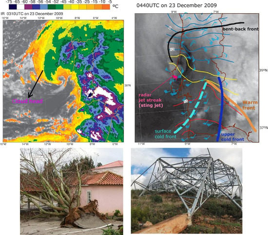
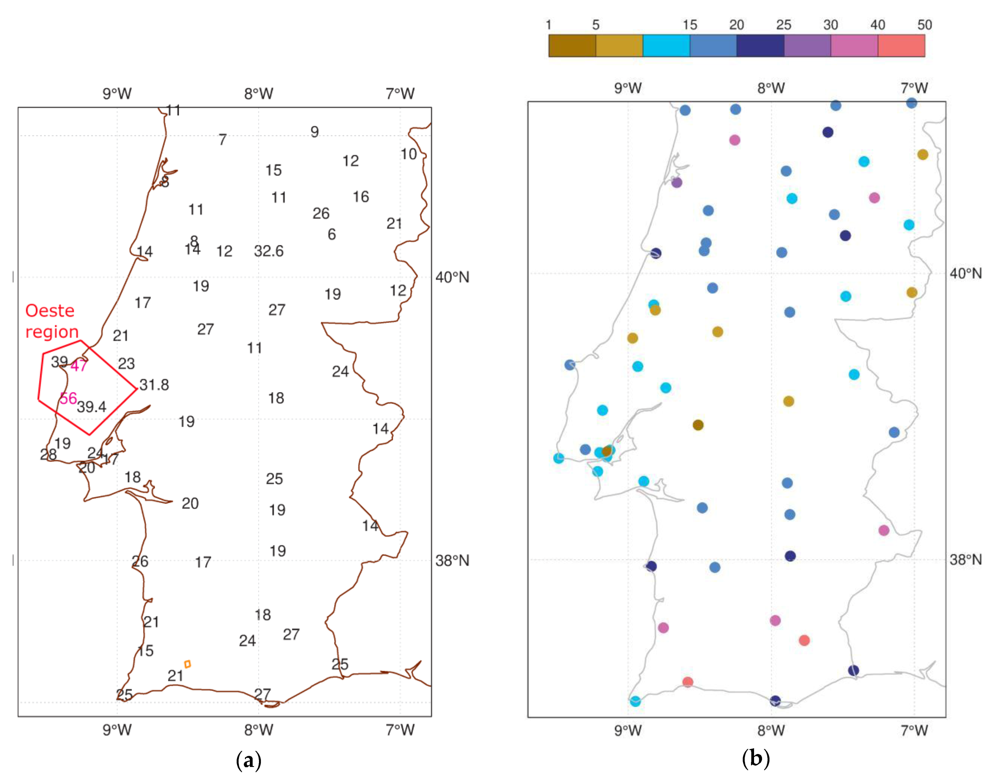
3.1. Surface Observations and Damage Reports

On 23/12/2009, wind gusts exceeding 28 m s⁻¹ were recorded by several stations in central mainland Portugal. However, during a short period between 04:30 UTC and 05:00 UTC, in a localized region no more than 50 km × 25 km (marked in Figure 1a), the wind was particularly strong. In this area (Oeste region), greenhouses, vegetation, public lighting, telecommunications, vehicles, houses and a camping site were severely damaged, causing a few displaced families. Fortunately, possibly because the event occurred in a relatively sparsely populated area, before sunrise during winter, there were only a few injured and no fatalities. More than 150 km of electrical cables were damaged and 15 power towers were destroyed. As a result, roughly 350,000 customers were left without electricity for several days. In the most affected municipality, out of a total of 600 ha of greenhouses, 250 ha were completely lost, and 250 ha were severely damaged. Further, 350 ha of pine trees and 150 ha of eucalyptus were affected, and 2500 trees fell or were uprooted, causing the closing of several roads. In the Oeste region, the economic losses were estimated to exceed EUR 100 million. In this area, two IPMA stations measured wind gusts at or slightly above 39 m s⁻¹ (Figure 1a), whereas a REN anemometer recorded 47 m s⁻¹ (at 60 m height), and a private anemometer measured 56 m s⁻¹, before being destroyed.

In southern Portugal, the second most affected area, near Portimão, 13 REN power towers were also destroyed (see Figure 1a and Figure S5e). According to REN, these towers (as those of the Oeste region) were designed to withstand up to 46 m s⁻¹ winds, and it was the first time in 60 years that such destruction occurred. In southern Portugal, IPMA stations registered 10-m wind gusts on the order of 21 to 27 m s⁻¹, and precipitation above 40 mm (in 6 h) was recorded (Figure 1b), mostly due to the thunderstorms that affected this region between 01:00 UTC and 05:00 UTC (Figure 1c). On the other hand, in the Oeste region, between 00:00 UTC and 06:00 UTC, the accumulated precipitation varied between 10 and 25 mm (Figure 1b).

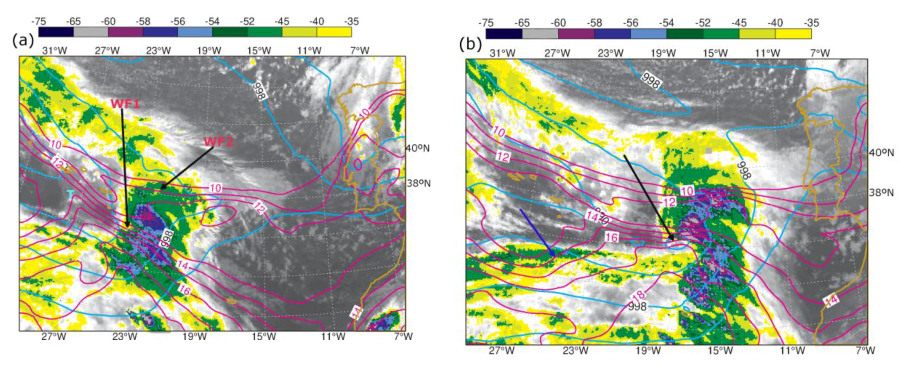
3.2. Synoptic Background of Windstorm Xola

During this episode of damaging winds, the windstorm Xola underwent a rapid deepening of 20 hPa in nearly 10 h, between 18:00 UTC on 22/12/2009 and 04:20 UTC on 23/12/2009, according to the ECMWF model and surface observations (Figure 2). The most rapid intensification occurred between 00:00 UTC and 04:20 UTC. At 04:20 UTC, the mean sea level pressure (MSLP) reached a minimum of 969.4 hPa, at the coastal station of Cabo Carvoeiro (see location in Figure 1d). In the next hour, as windstorm Xola crossed mainland Portugal from southwest to northeast, the central pressure rose to 979 hPa (Figure 2).

On 22/12/2009, an occluding extratropical cyclone was visible in the North Atlantic (Figure S6a,b), centered over the Azores archipelago (Figure S6c). The windstorm Xola formed over the warm front (labelled WF1) of this cyclone near its triple point (marked with a circle). This analysis also depicts a second warm front (labelled WF2), associated with the depression (T) that affected Iberia at 06:00 UTC (Figure S6). It will be shown that WF2 will play a role in the life cycle of the windstorm Xola. Moreover, Xola originated ahead of a dry intrusion, visible on the WV6.2 satellite image at 12:00 UTC on 22/12/2009 (Figure 2). The dry intrusion west of the comma cloud reflects a tropopause fold, which is identifiable by high values of potential vorticity (PV) in the ECMWF analysis. This tropopause fold was associated with an upper-level trough (shown later). Figure 2 also depicts an intense jet streak at 300 hPa south of the PV maximum, showing that Xola developed beneath the left exit region of an upper-level jet streak. Carroll [51] discussed how cyclogenesis is favored in this location, because an upper-level divergence develops in this region in response to the upward motion associated with an ageostrophic circulation.

At low levels, an area of strong baroclinicity (highlighted by the TFP at 925 hPa) and convergence (−10 to −15 × 10⁻⁵s⁻¹), associated with the occluded front and WF1, was present beneath the dry intrusion (Figure 2 and Figure S6c). The other warm front, WF2, was also identifiable by a weaker maximum of the TFP, and by a wind veer depicted by the ASCAT product. South of WF2, over the cloud band, wind speed ranged from 25 to 30 kt (Figure S6c).

At 12:00 UTC, the above-mentioned warm fronts were clearly delineated by a sharp contrast in θ_w, at 925 hPa (Figure 3a). Associated with the surface trough and with WF1, low-level cyclonic vorticity (>10 × 10⁻⁵s⁻¹) was present (not shown) along the region of TFP maximum (see Figure 2 and Figure S7a), co-located with the low-level convergence (Figure 2). Rogers and Bosart [52] showed that the development of low-level convergence, co-located with a preexisting low-level cyclonic vorticity area, contributed to the explosive development of two oceanic cyclones.

At this time, the warm sector was characterized by warm and very moist air (θ_w ranging between 16 and 19 °C), and by large potential instability (PI < −4 °C; see Figure S8a). An extensive cloud band was evident, where the highest and coldest tops (<−54 °C) were visible over the eastern quadrant of the warm sector and north of the WF1 (Figure 3a).

At 18:00 UTC, both the θ_w gradient and the TFP along WF1 intensified (Figure 3b and Figure S7b). South of this warm front, there was also an intensification of the southwesterly winds at 925 hPa, with wind speeds ranging from 50 kt (25 m s⁻¹) to 65 kt (Figure S7). North of WF1, the wind speeds were much weaker (Figure S7b), causing a reinforcement of the low-level convergence (Figure S9b) and cyclonic vorticity (>20 × 10⁻⁵s⁻¹) along WF1 (Figure S9c). These conditions lead to intense deformation along WF1, which, according to the Miller’s Frontogenetic function (see Equation (5) of Roger and Bosart [52]) promotes frontogenesis. Moreover, the small surface low (indicated by the black arrow in Figure 3b) favored not only an intensification of the θ_w gradient, but also the bending of the θ_w isopleths, leading to the onset of the cold front. A second maximum of TFP (>4 °C/(100 km)²) marking WF2 was also visible at 18:00 UTC. Along this front there was also a wind shift with southwesterly winds to the south, and weaker easterly winds to the north of WF2 (Figure S7b), causing low-level convergence.

It is relevant to mention that the strong southwesterly winds at low levels south of WF1 (Figure S7b) promoted strong warm advection, mainly in the eastern quadrant of the warm sector, which favored strong upward motion. This condition, together with the potential instability in this area (Figure S8b), supported deep convection, as suggested by the highest and coldest tops (<−60 °C) observed at this time. The deep convection on the eastern flank of the cyclone center may have contributed to reinforcing the deepening of the surface low, via convective latent heat release. Some studies have suggested that this diabatic forcing contributes positively to cyclogenesis [53]. The satellite images also revealed high and cold tops just north of WF1, coincidently with a maximum of low-level convergence (Figure 3b and Figure S9b). Notice also that at 18:00 UTC the cloud pattern was in the shape of a comma, which is indicative of strong upper-level vorticity advection [52], and suggests that the Xola storm was deepening [54].

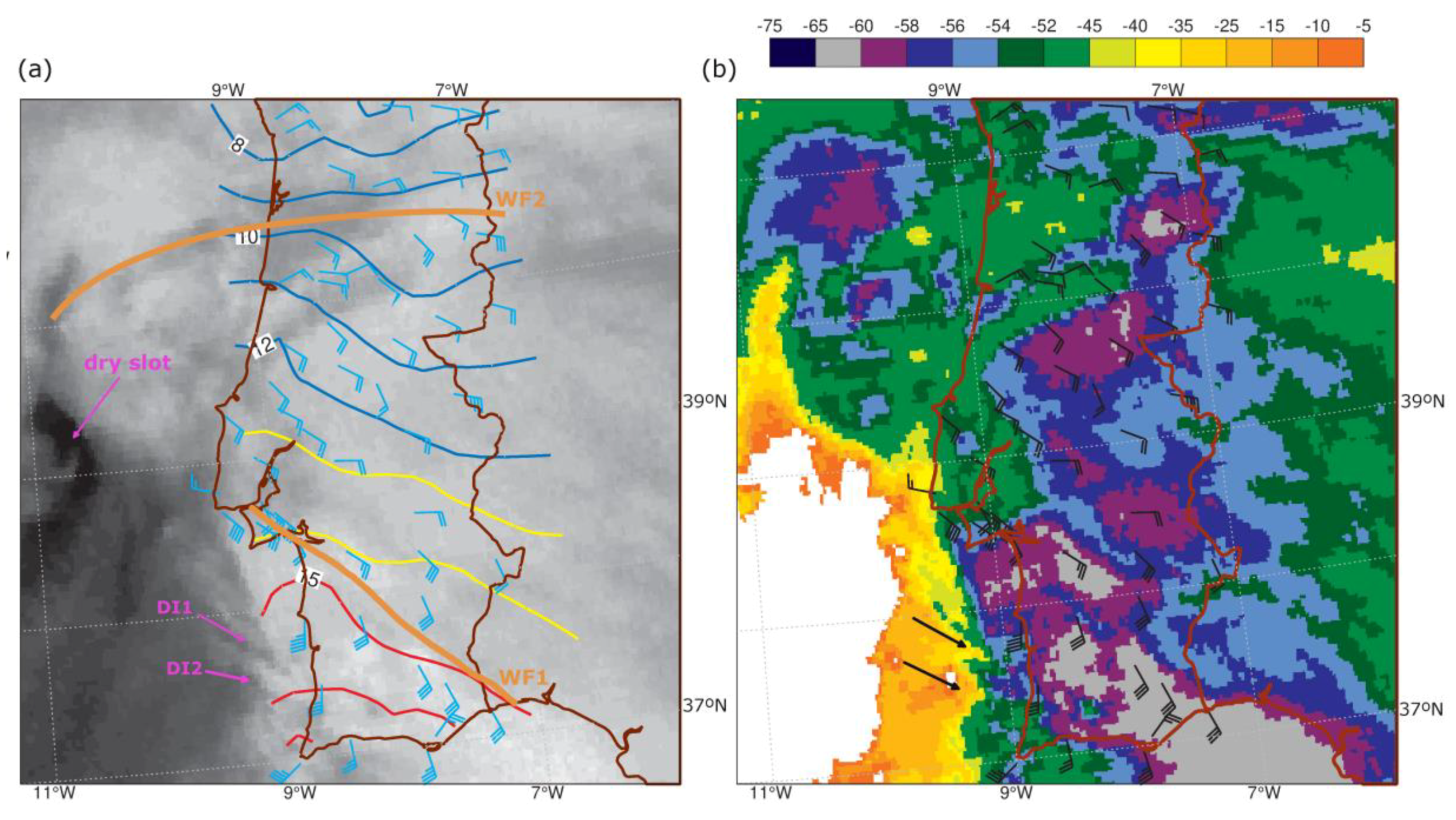
3.3. The Cloud Head and the Split-Cold Front

In the next couple of hours, as Xola approached the coastline, satellite images revealed a prominent cloud head and a dry slot, as illustrated in Figure 4. These features are characteristic of cyclones that follow the evolution described in the S-K model [1]. Moreover, at 00:00 UTC, the satellite images of windstorm Xola resembled stage III of the S-K model (compare Figure 4 and Figure S1). However, this windstorm presented two features that were not characteristic of the S-K conceptual model. The first one was a double warm front structure, and the second was a split cold front, later discussed.

At 00:00 UTC on 23/12/2009, a double warm front structure was delineated by the TFP, with the fronts depicted both at 925 hPa and 850 hPa (Figure 5a). Such a structure was also found in the windstorm Gudrun [8]. The TFP and θ_w isopleths at 925 hPa showed that WF2 was encircling the cyclone center, although this encircling was less obvious at higher levels. Figure 4b and Figure 5b displayed high cloud tops (<−60 °C) in association with WF2, consistent with the heavy precipitation (>30 mm/6 h) that occurred in central and northern regions of mainland Portugal (see Figure 1b) over the next 2 h. At 00:00 UTC, WF1 appears to start to encircle the cyclone center. This was delineated by the θ_w isopleths, mostly at low levels (Figure 5a,b).

Figure 5a and Figure S10a showed that the strongest winds at low levels occurred in the warm sector and along WF1, with wind speeds attaining 70 kt (35 m s⁻¹) at 925 hPa, and 80 kt at 850 hPa. Ahead of WF1, winds were weaker, favoring the development of strong low-level convergence. This convergence reached a maximum (<−50 × 10⁻⁵ s⁻¹) in the northeastern flank of the cyclone center, which probably contributed to the development of a narrow band of cold cloud tops in this area (Figure 5).

At 00:00 UTC, the cold front was identifiable by a strong gradient of θ_w, and by a TFP maximum and a vorticity maximum at low levels (Figure 5a,b and Figure S10). However, one could perceive a separation between the position of the cold front in the lower troposphere (Figure 5a,b) and in the middle troposphere (Figure 5c), suggesting the structure of a kata-cold front (see Figure S11). This configuration is sometimes referred to as split cold front, due to the existence of an upper-cold front (UCF) ahead of the surface cold front [21,24,25]. The structure of the cold front in Xola presented several features that were typical of the conceptual model of the split cold front. One of these features was the low relative humidity in the middle troposphere, above the surface cold front (SCF), which extended more than 100 km ahead of it (Figure 5 and Figure S10b). Behind the UCF, the relative humidity decreased abruptly (Figure S10b). For this reason, the UCF is sometimes named the humidity front [4,24]. The sharp contrast in relative humidity marking the upper cold front was also visible in the cross-section displayed in Figure S12a, where this signature was visible in the layer 500–800 hPa, and it was also marked in the θ_w gradient. This cross-section also revealed that between the SCF and the upper cold front, air with lower θ_w overran the moist high-θ_w air of the warm conveyor belt, leading to potential instability, which was also depicted in Figure S8c. This overrunning is a consequence of the dry intrusion, identifiable in the WV6.2 imagery (Figure 4a and Figure 5d) and in the PV maximum illustrated in Figure 5d. The presence of shallow clouds over the SCF and behind the upper cold front in the warm sector is also noticeable, where the cloud top temperature ranged from −3 °C to −25 °C (Figure 5b and Figure S12b). This area between the SCF and the humidity front, where cloud tops were generally lower than 3 km, is termed the shallow moist zone [22,24,25]. This is another characteristic feature of the split cold front. The clearance of middle- and upper-level cloud in the shallow moist zone is caused by the dry intrusion [22,24].

Ahead of the upper cold front, a tongue of high θ_w at 700 hPa (Figure 5c) was also visible, characterized by large potential instability (Figure S8c). These conditions contributed to the development of deep convection, which affected the southern region of mainland Portugal, as will be shown in the next section. The abrupt decrease of the cloud top temperature to values below −50 °C denoted the position of the upper cold front (Figure S12b). Moreover, a wide band of cold cloud tops was visible ahead of the UCF, where the coldest tops varied between −54 °C and −70 °C (Figure 5b), suggesting the presence of cumulonimbus anvils. This was confirmed by the overshooting top product (Figure S13) and radar observations (Figure S14), and is consistent with the lightning activity registered between 01:00 UTC and 05:00 UTC (Figure 1c). The frontal structure of windstorm Xola resembled the conceptual model of diffluent-type cyclogenesis (Browning [2]; their Figure 5), where dry intrusion in the presence of a diffluent trough produced a split cold front.

Previous studies claimed that strong winds in middle troposphere could be advected down by a secondary circulation, due to frontolysis in the frontal-fracture region, explaining the location of the sting jets [17,19]. At 00:00 UTC and 03:00 UTC, the Petterssen’s Frontogenesis function revealed weak frontolysis on the southwest flank of the cyclone, in the levels between 500 hPa and 850 hPa, as illustrated for 800 hPa in Figure S10c,d. These figures also displayed strong frontogenesis along the two warm fronts and the UCF, as would be expected [11].

Figure 5 also shows that the cyclone, with a central pressure of 980 hPa at 00:00 UTC, developed in the close proximity of two upper-level jets (J1 and J2). This factor is known to reinforce the cyclogenesis [23]. The development of upper-level divergence in the left exit of the jet streak, due to an upward motion caused by an ageostrophic circulation, was previously discussed. The right entrance of the jet streak (J2) is also prone to upper-level divergence. Therefore, the interaction of the upper-level forcing with the low-level baroclinicity contributed to the deepening of storm Xola in the next few hours.

3.4. The Bow Echo and Mesovortex

At 02:30 UTC, the above-mentioned upper cold front was identifiable both on satellite (Figure 6) and on radar (Figure 7a). In the water vapor channel, the leading edge of the dry intrusion represented the upper cold front position (Figure 6a). In the IR image, the upper cold front was marked by the sharp transition between the band of cold cloud tops and the shallow clouds that were observed to the west (Figure 6b). In association with the humidity front (or UCF), radar observations displayed a line of cloud tops exceeding 7 km in southwestern Portugal at 02:30 UTC, moving eastwards (Figure S14). In the region of Sagres and Portimão, very high cloud tops (>10 km) are visible in association with a bow echo, as will be discussed later.

Figure 6a also displays the presence of a moist and warm air mass (surface θ_w > 15 °C) in a southerly flow, with winds gusting from 30 kt to 45 kt south of the warm front, WF1. To the north of WF1, southeasterly winds prevailed, and were causing a convergence line along WF1 (marked by the orange line).

In addition to the synoptic forcing described previously, the atmospheric environment was characterized by large potential instability (Figure S8c), a meagre convective available potential energy (150–300 Jkg⁻¹, based on ECMWF) and strong wind shear. The wind shear was computed from the vertical wind profile derived by the radar [55], and revealed unidirectional shear above 2.5 km, and small veering below. The vertical bulk shear was of 22.5 m s⁻¹ for the 0–2.5-km layer, and 25 m s⁻¹ for the 0–5-km layer, slightly above the values reported in other studies [29,35]. This overall setting resembled the one described by Locatelli et al. [26], and is prone to the development of a squall line.

Furthermore, at 02:30 UTC, the WV image showed the presence of dry air finger patterns (identified by DI in Figure 6a) just behind the UCF, suggesting local entrainment of drier air in the rear of the UCF. These finger patterns were co-located with lowering tops (Figure 6a,b), consistent with evaporative cooling and descent. This appears to be confirmed by the presence of an inflow to the rear of the UCF, identified on Doppler observations at an altitude of about 3600 m (Figure S15d). Browning et al. [56] identified rear inflows associated with dry air fingers as part of a mesoscale transverse frontal circulation. This type of circulation has been associated with the intensification of the squall line [57]. By 02:30 UTC, a bow echo embedded in a squall line was identified close to the southwestern tip of Mainland Portugal (Figure 7a,b), slightly upwind of the site where several power towers were completely destroyed 8 min later (Figure 7c). The width of the damage swath was, at least, 2.6 km, and the length remained unknown since these winds affected an area without significant structures that could exhibit traces of damages, apart from the ones that were referred to. These power towers were well maintained and were built to withstand winds up to 46 m s⁻¹, which suggested that near-surface winds may have exceeded this value.

This squall line was a prolific MV producer; however, this study focuses on the MV that caused the damaging winds. The damaging bow echo propagated from Sagres to the northeast, between 02:07 UTC and 02:47 UTC (Figure 7c, Figure 8 and Figure S15). The MV associated with this bow echo was firstly observed by 02:07 UTC (not shown), between altitudes of 1.5 and 7.5 km, with a maximum rotation strength near an altitude of 3.5 km (Table S1). By this time, the MV presented the weakest rotation and the highest diameter (>11 km) of the entire observation period. A rear-inflow notch (RIN) and a rear-inflow jet (RIJ) became noticeable only 10 min later, by 02:17 UTC (Figure S15c,d). The rotation in the MV increased slightly, but the diameter remained larger than 11 km (Table S1). At 02:27 UTC, the collocation of RIN and RIJ was visible along the second tilt (2.8 km altitude) (Figure 8a,b) and third tilt (5.7 km altitude). Moreover, between 02:17 UTC and 02:27 UTC, the MV rotation intensified (azimuthal shear nearly doubled), and its diameter decreased to less than half (Table S1). The vortex contraction was also confirmed at higher levels (Table S1). By 02:27 UTC, the magnitude of the outbound values observed up to an altitude of 3 km was in the range 21–28 m s⁻¹, whereas the magnitude of the inbound values was in the range 5–10 m s⁻¹. Note that the MV was monitored to the southwest of the radar, and that the squall was approaching it. Therefore, the outbound winds (away from the radar) corresponded to inflow relative to the MV. Thus, on a storm-relative frame, the observed inflows, located in the northern bound of the MV, were stronger than the observed flows located in the southern bound of the MV.

Between 02:27 UTC and 02:36–02:37 UTC, the RIN and RIJ remained co-located and strengthened (Figure 8c,d), and the MV continued to intensify (azimuthal shear four times larger than before). The MV reinforcement was associated with a reduction of the diameter, and with an increase in the difference between maximum outbound and inbound velocities. By 02:36 UTC, 2 min before the reported damages, the low-level couplet was 2 km upwind of the area of the damages, and it was identified on radar at an 800-m altitude, or 700-m height (Figure 8f,g). In the 1.5° tilt, the RIJ was identified proceeding from the rear to the MV rotation center, with increasingly higher winds along with the rear inflow (Figure 8d), at speeds from 11 m s⁻¹ in a location 9 km to the rear of the center (2.2 km altitude) up to 16.5 m s⁻¹ close to the center (2.0 km altitude).

The Doppler winds, relative to the ground (Figure 8g) in the MV center and the surroundings (including both the north- and southbound parts of the MV), revealed southwesterly winds (approaching the radar), due to the fast advection of the storm to the northeast. The MV revealed significant asymmetry, with winds exceeding 45 m s⁻¹ in the southbound part of the MV, and just 20 m s⁻¹ observed in the northbound part, only 2 km far (not shown). The situation was similar at a 0.8 km altitude, with speeds of 25 m s⁻¹ in the northbound part and aliasing signatures (see Appendix A) in the southbound part of the MV (Figure 8g). It was estimated that radial winds of at least 56 m s⁻¹ were observed in the southbound area. The RIJ is a descending jet, and this meant that along a part of its trajectory, towards lower levels, especially when observed by the lowest tilt, only a fraction of the magnitude of the descending flow could possibly be observed. Considering this, it is conceivable that winds at or above 56 m s⁻¹ may have affected the surface, and produced the reported damages. By 02:47 UTC the MV rotation embedded in the bow echo was still observable (Figure S15e,f), but the vortex circulation was weakening (Table S1).

The preceding observational evidence sustains that the strong winds observed at 700 m resulted from the merging flows of the southbound part of the MV and the RIJ. When the RIJ, which was being observed at the second tilt, was superimposed over the lowest tilt observations (Figure 8f), it became clear that the jet was feeding the southbound part of the MV. This result agrees with previous studies that showed that the most damaging winds associated with an MV often occur when this superimposition takes place [29,36]. In the current event, though, the contribution of the RIJ was major. Indeed, the SRV values in the northbound part of the MV, at low levels, remained unchanged during the period 02:27–02:47 UTC, on the order of 23 m s⁻¹ (Table S1). However, the SRV values in the southbound part were on the order of 6 m s⁻¹ at 02:27 UTC, and 12 m s⁻¹ at 02:47 UTC, when the RIJ was not interacting with low levels, whereas by 02:37 UTC the SRV increased to 26 m s⁻¹ as the RIJ descended to low levels (Table S1). These results are consistent with the numerical studies, which showed the importance of the RIJ in the generation of damaging near-surface winds associated with bow echoes [58,59].

At the weather station of Portimão (see location in Figure 1d and Figure 7c), a sudden temperature drop of 2.5 °C and a pressure rise of 2.5 hPa was noticeable at approximately 02:30 UTC. These changes were accompanied by a wind shift and steep increase of the wind gust, nearly coincident with a sharp increase in the precipitation (Figure 9). A similar signature was also detected in the Sagres station 10 min before (Figure S16). The comparison of these signatures with the mesovortex’s trajectory indicates that these changes reflected the development of a surface mesohigh and cold pool, associated with the propagation of the MV embedded in the bow echo, as documented in previous studies [29,37,60]. On both stations, the southbound part of the mesovortex was associated with wind gusts in the range of 23–26 m s⁻¹.

3.5. Mesoscale Structure of the Cloud Head and the Sting Jet

3.5.1. Slantwise Convective Circulations

Some studies claimed that CSI plays a key role in the sting jet formation [7,10,11,12]. A formal definition states that CSI occurs where MPV is negative, and conditional instability (CI) and symmetric instability (SI) are absent [61]. Figure 10a displays the MPV in the layer 800–950 hPa, where these criteria are fulfilled. This figure portrays the presence of conditional symmetric instability in the western flank of the cyclone and behind the SCF, revealing conditions prone to slantwise convection [61].

As windstorm Xola was approaching land, between 03:00 and 03:40 UTC, the dry slot presented a southwest-northeast orientation, as the cloud head started to encircle the cyclone center from the south (Figure S17a,b and Figure 10b), suggesting that windstorm Xola was close to reaching the minimum central pressure [3]. The absence of cloudiness in the dry intrusion region, and the presence of low clouds in the shallow moist zone, behind the humidity front (or UCF), is also noticeable (Figure 10b,c and Figure S17). The SFC is located just behind the shallow clouds, which are approaching Sines (Figure 10c). This explains both the absence of precipitation and the occurrence of light precipitation in southern Portugal within the following few hours, as illustrated in Figure 9, Figures S16 and S18. The radar images revealed a hook-shaped reflectivity pattern associated with the cloud head, and the absence of backscattering between the cloud head and the SCF, due to the dry intrusion (Figure S17b,c and Figure 10d).

Ahead of the cloud head tip, an arc-shaped cloud at 03:40 UTC is noticeable (Figure 10c,d). This cloud feature, which started to be identifiable 30 min before (Figure S17c,d), reached its maximum extension by 03:40–03:46 UTC (Figure 10c,d) and dissipated after 04:10 UTC. Previous studies have also identified arc-shaped clouds ahead of the cloud head tip [3,62], and hypothesized that these shallow cloud features were the result of boundary-layer convergence lines. At 03:40 UTC, the hooked cloud head presented a banded structure, with at least three relative maximum reflectivity lines alternating with the relative minimum reflectivity lines (Figure 10d). Previous authors [3,62] attributed this banding to stacked slantwise convective circulations, formed by ascending and descending branches (see Figure 10e). These authors also claimed that the ascending parts are cloudy with precipitation, and collectively responsible for the hooked tip of the cloud head. They also pointed out that descent dominated in both branches where the cloud tops started to progressively drop (Figure 10e), and that the descending flows continued in the dry slot area. The precipitation that fell into the dry air of the descending branches of the circulations suffered evaporation, which would contribute to the reinforcement of the descending flow. These descending branches corresponded to multiple SJs, and would be responsible for surface-damaging winds just ahead of the tip of the cloud head, as well as for the generation of convergence lines, which contributed to the formation of the arc-shaped cloud previously mentioned [62]. These damaging winds were referred to as the sting jet by Browning [3].

The banded structure in the cloud head portrayed in Figure 10d was possibly due to the release of CSI (Figure 10a), as supported by other studies [10,11]. It is also noteworthy that radar observations were used to estimate the advection of the reflectivity bands for nearly two hours (Figures S17c,d, S19b and S21b). These bands were found to be moving at the same speed and in the same direction as the windstorm Xola. Thus, these bands did not propagate relative to the environmental flow. This indicates that these bands were associated with the CSI [61].

From 0310 UTC to 0410 UTC, the ground-relative travel speed of the arc-shaped cloud was 29 m s⁻¹ from 240°, as estimated from the radar imagery, which was higher than the travel speed of the cyclone, estimated as 22 m s⁻¹ from 244°. By 03:46 UTC (Figure 10f) and in the following moments (not shown), Doppler radar observations showed that this arc-shaped pattern propagated downstream (to the northeast) of the strongest wind flow measured on the radar. By this time, this flow was particularly strong at the tip of the cloud head, with a maximum velocity of 52.2 m s⁻¹ relative to the ground (not shown), and a maximum SRV of 34.2 m s⁻¹ (Figure 10f). Along with the arc-shaped pattern, the largest magnitude of the SRV (and of V) was observed at the apex (Figure 10f), downwind of the tip maximum winds. These large values of SRV at the tip revealed the large relative advection speed of the southwesterly flow exiting the tip, suggesting that the condensation of the cloud head was evaporating at a substantial rate, as explained by Browning [3]. Furthermore, as will be discussed ahead, the strongest winds at ground level, as well as the most severe damages, were observed 40–50 min after this arc-shaped pattern propagated over the locations. These results agree with the conceptual model of Browning and Field [62] (see Figure 10e), suggesting the onset of the strongest winds behind a convergence line that generated the observed arc-shaped cloud.

Figure 11 shows the TOPS radar product at 03:40 UTC and 04:40 UTC. In the cloud head, when Xola was still offshore, the cloud tops descended progressively and sharply towards the edge of the cloud head tip. At 03:40 UTC, the cloud tops decreased from an altitude of 6000–7000 m, in a region 50 km upwind of the tip, to an altitude of 3800 m by the tip (Figure 11a,c). One hour later, when the tip was over the Oeste region, the progressive lowering of the tops prevailed, with the exception of the fact that the cloud tops were now shallower on average (Figure 11b,d). At 04:40 UTC, the tops decreased from 5000–6000 m to less than 2000 m, along the same section considered before (Figure 11b,d). This significant lowering was also confirmed by the IR 10.8 imagery (compare Figure 11a and Figure 10b). Note also that the observed lowering of the cloud tops of Xola, observed throughout this 1 h period, was confined to the cloud head region, more specifically, to the southwest of the cyclone center. It is also interesting to notice the coincidence between the alternating higher and lower cloud tops and the band structure in reflectivity (compare Figure 11 with Figure 10c,d). This is coherent with the descent of the branches of slantwise circulations, interleaved with ascending branches, where the cloud tops rapidly lowered due to the termination of the ascent, and there was a rapid onset of evaporation of cloud, according to the conceptual model of Browning [3].

In the period 04:35–05:00 UTC, the proximity between the cloud head tip and the radar enabled a detailed look at its structure. The SRV pattern of the cloud head tip is shown in Figure 12, at altitudes between 2900 m (at 04:37 UTC) and 2500 m (at 04:57 UTC), and from second tilt observations, and at a 700-m altitude (at 04:46 UTC) from the lower tilt observations. At 04:37 UTC, a jet streak pattern was noticeable, and three aligned signatures of velocity were distinguishable along with the jet streak (Figure 12a). These signatures were identified by letters “S” and “F”. F Lines denoted the axis of faster storm-relative velocities, and line S represents the axis of slower storm-relative velocities, towards the radar. This interleaved structure of relative maximum and minimum storm-relative velocities was observed for at least 30 min (Figure 12 a–c). These signatures were also observed at a 700-m altitude, at 04:46 UTC (Figure 12 d), despite being less clear than in levels above (compare with Figure 12b). Besides, this three-dimensional structure was coherent throughout these 30 min. These kinematic signatures, with alternating faster and slower air flows, within the cloud head tip, may correspond to the stacked slantwise convective circulations, as proposed by Browning [3].

An additional interesting aspect can be noted in the comparison of the signatures at 04:46 UTC and 04:47 UTC (Figure 12b,d). The highest tilt (Figure 12b) scanned the cloud head tip approximately 30 s later than the lowest tilt (Figure 12d). During this time, the cloud head propagated about 700 m northeastwards (at 22 m s⁻¹ from 244°), and therefore at 04:47 UTC the cloud head was already 700 m to the northeast of its position at 04:46 UTC. A careful analysis of the positions of the F and S signatures of SRV shows that, at 04:47 UTC, the axes of F or S were still slightly to the southwest of their corresponding locations at the lowest tilt (at 04:46 UTC). This was also found at other instants. Even if subtle, this fact suggests that the maximum (and minimum) relative SRV axis was inclined towards the outer part of the cloud head. Moreover, the superimposition of the F and S axes with descending flows over the reflectivity (Figure 12e) shows that faster descents (F1, F2) were co-located with minimum reflectivity, whereas the slower descent (S) was co-located with maximum reflectivity. These signatures are interpreted as evidence of slantwise convection.

It is also noteworthy that, according to the conceptual model of Browning, beyond the tip of the cloud head, in a cloudless area, descending airflows dominated in both branches of the slantwise convective circulations (Figure 10e). However, in windstorm Xola, as observed and schematically represented (Figure 12e,f), generalized descent was still identified within the cloud head, at the tip. As noted before, these descending branches have been associated with the descent of the SJ [7,9,10].

3.5.2. Sting Jet

At the coastal station of Cabo Carvoeiro (see its location in Figure 1d) during the first 4 h of 23/12/2009, a strong decrease of the MSLP (25 hPa) up til 04:20 UTC was observed, as the windstorm Xola approximated the Iberia. Between 02:10 UTC and 03:50 UTC, a marked increase in temperature was also noticeable, as the warm conveyor belt approaches. Before that instant, the wind was coming from the south quadrant. Between 03:00 UTC and 04:50 UTC, as the cyclone center approaches, the wind rotates progressively from SE to NW, and the wind gust increases from nearly 15 m s⁻¹ to 39 m s⁻¹. In this time interval, the first maximum of the wind gust, 35.5 m s⁻¹ from SE, was registered at 04:00 UTC. By this time, the pressure gradients were strong around the eastern flank of the depression, as illustrated in Figure S19a. Thus, the gradient wind, estimated at 28 ± 2 m s⁻¹, was sufficient to explain a large part of the strength of the surface winds. A further enhancement of the wind strength in this location may be caused by the transfer of momentum down to the surface, promoted by shallow convection (Figure S19b). This is coherent with the rapid decrease of temperature and relative humidity around this time, which may be associated with the dry cold air brought down by convective downdraughts. This mechanism, of transferring high momentum downwards, was previously documented [18,63].

At Cabo Carvoeiro, the maximum wind gust, 39 m s⁻¹ from 300°, was registered by 04:50 UTC, 30 min after the minimum MSLP had been attained (Figure 13). This peak gust coincides with the passage of the cloud head tip over the station, as will be shown, and was accompanied by light precipitation, as illustrated in Figure 13c. After 05:00 UTC, the relative humidity decreases as the dry intrusion approaches the station, and wind gusts decrease as the depression weakens and moves northeastward.

Between 04:30 UTC and 04:50 UTC, even when the cloud head tip was closer to the radar, it was not possible to perform a very detailed three-dimensional analysis, due to the relatively coarse vertical resolution. However, it was possible to identify a jet streak pattern at the two lowest tilts of the Doppler velocity (V) radar scan (Figure S20). Specifically, at 03:46 UTC, Doppler observations detected this jet streak below an altitude of 900 m. Figure 14a depicted this jet between 39° N and 39.5° N. In the core of the jet at that altitude, the wind speed was so high that V exceeded the Nyquist velocity. Magnitudes as high as 54.5 m s⁻¹ were being observed (corresponding to 60 m s⁻¹, as shown in Appendix A). V and reflectivity observations also showed that the jet streak was always co-located with the reflectivity tip of the cloud head, and that V increased progressively towards the tip end (Figure 14a,b). The jet streak was better defined at the lower levels (0.1°) during this 04:30–04:50 UTC period. At the lower tilt, the jet streak was observed at altitudes between 450 m and 900 m, depending on the range to the radar site and observation time. In the 1.5° tilt, the jet streak was observed between 1700-m and 2700-m altitudes. The total wind speed was estimated from the two tilts (see Appendix A), but the higher speeds were consistently observed in the lower tilt, as shown in Figure 14c.

The spatial distribution of the strongest near-surface wind gusts showed that the two IPMA stations (Cabo Carvoeiro and TV), where the maximum gusts (>39 m s⁻¹) were recorded, were located near the edges of the low-level jet streak. Moreover, these maximum gusts were observed when the jet streak was closest to them. The REN anemometer at a height of 60 m, located at the edge of the jet streak, measured a wind speed of 47 m s⁻¹, whereas a private anemometer located beneath the jet streak core recorded 56.4 m s⁻¹, before being destroyed (Figure 14). The power towers located near the jet streak were destroyed in the period between 04:34 UTC and 04:48 UTC, according to REN reports. These facts reveal that there was a transfer of strong momentum from the low-level jet (between 450 and 900 m), observed on radar, to ground level.

Figure 15 shows the superimposition of satellite imagery with observations of 10-m wind gust, MSLP and surface θ_w, illustrating several interesting features. In the cloud head, three major cloud filaments can be identified, and, between the cf filament and the other two, the signatures of dry air aligned with progressively lowering tops were apparent. The airmass RGB reveals that these signatures correspond to dry descending stratospheric air (not shown). The close proximity of this dry airflow, of stratospheric origin, with the progressively lowering cloud tops suggests the presence of a downward-oriented flow within the cloud head. It also provides favorable conditions for the evaporation of the cloud’s filaments. Finally, Figure 15 shows that the low-level jet detected by radar is located at the end of the cloud head tip, just ahead of the evaporating cloud filament and the descending dry air. These results are consistent with the findings of Browning et al. [18], and strongly suggest that this jet was a sting jet. Between 04:40 UTC and 04:50 UTC, the reflectivity cloud tip passes over the station of Cabo Carvoeiro, explaining the strongest gust (39 m s⁻¹) observed during this interval (see Figure 13, Figure 14 and Figure 15 and Figure S21). Browning et al. [18] demonstrated that convective showers are responsible for the downward transfer of momentum from the low-level jet to the surface. Moreover, the sounding based on ECMWF reveals low Richardson numbers (<0.26) below altitudes of 2500 m in this area (not shown), thus promoting the shearing instability and turbulent transport of high momentum to the surface.

3.6. Warm Seclusion

After the maximum gust in the Oeste region was observed at the IPMA stations, between 04:40 UTC and 04:50 UTC, the cloud head continued to wrap around the cyclone center as the windstorm Xola moved northeastwards. By this time, a cyclonic circulation on the eastern flank of windstorm Xola was evident, with stronger gusts (>35 kt) on the southeast flank, in the dry slot region (Figure 15). This circulation promoted deformation, contributing to the onset of warm seclusion. In the next hour, a weakening of the filament cf was visible, along with a reinforcement of the other two filaments (compare Figure 15, Figures S21a and S22). At 05:40 UTC, the surface low was centered in the Coimbra region (see Figure 1d), where the minimum MSLP was nearly 981 hPa. In the next two hours, the cyclone moved eastwards and continued to weaken (Figure 16). At 07:40 UTC, the cyclone presented a warm core with a diameter of 70–80 km, centered near the station of Covilhã, revealing the warm seclusion (Figure 16b). At this station, the MSLP minimum was attained around 06:20 UTC, after a pressure fall of 20 hPa over the previous 6 h. Nearly 40 min later, the relative humidity dropped sharply with the arrival of the dry intrusion (not shown). Up til 07:40 UTC, the surface θ_w increased 2.5 ℃, attaining a maximum of 13.5 ℃. At this time, near the cyclone center, a warm anomaly was visible, with the warm air entirely surrounded by colder air, corresponding to warm seclusion. However, it is interesting to note that this warm core presents characteristics distinctive from other cases reported in previous studies. In fact, the warm core delineated in Figure 16 was considerably smaller than that of the New Year’s Day storm [6] and of the Great storm [3], which had diameters of 150–220 km, which is consistent with the smaller size of the windstorm Xola. Moreover, the warm core of Xola had an asymmetric structure, since θ_w decreased 3 °C in the north direction but decreased less than 1 °C to the south, within a distance of 25 km from one another (Figure 16b). This warm core was also considerably weaker than that met by Browning [3], who found a gradient twice as strong.

Note that contrarily to the Great Storm, windstorm Xola presented a double warm front structure, and the warm bent-back front was formed from WF2 (compare Figure 17 with Figure 2 of Browning [3]). In the two hours previous to the warm seclusion, the presence of high θ_w (>15 °C) air was visible to the south of WF1 (Figure 15). In addition, the passage of SCF was marked by a soft decrease of θ_w, consistent with the conceptual model of the split cold front (Browning and Monk [24]). Consequently, even after the passage of the SFC (Figure 15, Figure 16 and Figure 17), south of the low center, high θ_w air was being advected by the cyclone’s circulation. These conditions explain why the warm core of windstorm Xola was weaker than that of the Great Storm.

4. Conclusions

On 23/12/2009 windstorm Xola struck mainland Portugal, creating damaging winds in two different regions. This study intends to understand the cause of these damaging winds. Windstorm Xola formed over the warm front of an occluding extratropical cyclone, and ahead of a dry intrusion caused by a tropopause fold that was associated with an upper-level trough. To the south of this dry intrusion, a strong upper-level jet streak was present, favoring the development of the storm just beneath its left exit region, characterized by upper-level divergence. At low levels and beneath the dry air intrusion, along the preexisting warm front, strong baroclinicity, cyclonic vorticity and convergence were feeding the storm’s development. Thus, the overlapping of upper-level and low-level forcings led to explosive development. Moreover, the presence of potential instability may also have contributed to the reinforcement of the storm. Windstorm Xola suffered a rapid deepening of 20 hPa in 10 h.

As Xola approached the Iberian coast, several features typical of Shapiro–Keyser (S-K) cyclones were highlighted by satellite, such as a prominent cloud head, a dry slot and a T-bone structure. Nevertheless, the windstorm Xola presented two features not characteristic of the S-K model: a double warm front structure (also found in windstorm Gudrun [8]) and a split cold front. This structure of the cold front develops when the dry intrusion overruns the warm conveyor belt, producing an upper cold front (UCF) more than 100 km ahead of the surface cold front [24], and is associated with the diffluent-flow type of cyclogenesis [2,21], which was the case of windstorm Xola.

This UCF established the environment for the damaging winds event that occurred in southern Portugal. By 02:30 UTC, observations suggested local entrainment of a drier air in the rear of the UCF, causing a descend inflow. This inflow has been associated with transverse mesoscale frontal circulations [56,57]. These frontal circulations in the UCF, the potential instability, and the presence of low-level moist and warm air associated with the warm conveyor belt, favored the development and intensification of a squall line. Moreover, this squall line, that progressed in an environment with strong vertical wind shear, was prolific in bow echoes and associated mesovortices. One of these bow echoes was associated with extensive damages to several power towers. The radar observations showed that the damaging mesovortex was already formed when a close RIJ became observable in its rear. As the mesovortex propagated northeastwards, its rotation increased as it contracted substantially. In the last 10 min before the onset of the damaging winds, the RIJ intensified and descended to low levels, contributing to feeding the southbound of the vortex and to the production of the strongest winds observed on radar. These winds affected ground levels, possibly at or above 56 m s⁻¹.

In the period 04:30–05:00 UTC, as the cloud head tip reached the Oeste region, a low-level jet streak was identified, with maximum values of Doppler velocity (V) exceeding 54 m s⁻¹ just 400 m above ground level. This jet streak, with an orientation of 280–300°, was always co-located with the tip of the cloud head as observed on reflectivity, and the V was observed to increase progressively towards the tip end. The progression of this jet streak through time was synchronous with the reports of severe damages and the strongest near-surface winds. This shows that the referenced low-level jet was impacting the surface, indicating that strong momentum was transferred down to the ground. Browning et al. [18] demonstrated that convective showers were responsible for the downward transfer of momentum, from a sting jet to the surface. Between 04:40 UTC and 04:50 UTC, as the cloud head tip and associated low-level jet propagated over the station of Cabo Carvoeiro, a 10-m wind gust of 39 m s⁻¹ and shower activity (~1 mm in 10 min) were recorded. These facts are coherent with the findings of Browning et al. [18].

Satellite images revealed major cloud filaments in the cloud head tip. Adjacent to or between these filaments, signatures of dry air (furrows) of stratospheric origin were identified, aligned with progressively lowering tops. As Xola was moving to the northeast, observations revealed the dissipation (evaporation) of the cloud’s filament located to the south of these furrows, and the reinforcement of the cloud filament to the north. Furthermore, the low-level jet and the strongest surface winds were observed at the end of the cloud head tip, ahead of these furrows, and at the leading edge of this evaporating cloud filament. It is also noteworthy to mention that nearly 40–50 min before the occurrence of the damaging winds in the Oeste region, an arc-shaped cloud was identified on radar and satellite, associated with the tip of the cloud head. Thus, the identification of this pattern may be useful in an operational forecasting environment.

The present observational study strongly suggests that the damaging winds in the Oeste region were caused by a sting jet. To the author’s knowledge, it is the first time that such phenomena occurred in Europe south of 40° N. It is also interesting to note that both the location and orientation of this strong low-level jet in windstorm Xola differed from those of sting jets in other windstorms. For instance, in the Great Storm, the strongest gusts attributed to a sting jet occurred in the dry slot, ahead of the cloud head tip (see Clark and Gray [14]; their Figure 4), and were embedded in a southwesterly flow, whereas in the case of Xola they occurred at the cloud head tip, and winds were westerly-northwesterly. These differences may be explained by the fact that the sting jet in Xola was observed in a later stage of the cyclone’s life cycle, compared to other storms [5,8]. This finding is consistent with the results of a climatological study by Parton et al. [13], done using a profiling radar, which found that sting jets at stage III of the S-K conceptual model occurred in the dry slot region, while those occurring at stage IV were located in the cloud head tip.

During landfall and one hour before the sting jet hit the Oeste region, the radar observations showed banding in the cloud head. It could also be seen that the cloud tops descended progressively and sharply towards the edge of the cloud head tip. Moreover, the kinematic structure of the cloud head tip revealed the presence of organized and coherent airflows, characterized by alternating faster and slower branches, which appeared to be inclined towards the outer part of the cloud head. These signatures were interpreted to be a consequence of stacked slantwise convective circulations, which is coherent with the release of moist symmetric instability, as diagnosed by the ECWMF fields. Despite the coarse horizontal resolution (25 km) of the ECMWF model at the time, its vertical resolution was only slightly coarser than that used by other studies [11,12], which stressed the importance of resolution in resolving CSI release.

To conclude, it is important to remember that SJs result from an airflow descending from the middle level in the cloud head into the frontal-fracture region, over a few hours, leading to near-surface strong winds [11,14]. Schultz and Sienkiewicz [19] claimed that frontolysis, and the resulting secondary circulation, must be strong enough and last long enough to advect strong winds aloft down to the lower troposphere. Other studies argued that CSI may enhance this frontal circulation, producing more rapid descent and greater accelerations [9,11,12]. Evaporation or sublimation of hydrometeors falling from the upper part of the cloud head may strengthen the descent [7,11,12], and convective downdraughts may contribute to transferring high-momentum air down to the surface [18]. Clark and Gray [14] mentioned that frontolysis may, in some storms, be sufficient to produce a sting jet, but in others, several mechanisms play a role. The results presented in this study suggest that frontolysis was not sufficient to explain the development of a sting jet in the windstorm Xola. They also sustain the idea that all the above-mentioned mechanisms may have contributed to producing damaging winds at the surface, associated with the sting jet, with special emphasis on CSI and evaporative cooling.

References

1. Shapiro, M.A.; Keyser, D. Fronts, Jet Streams and the Tropopause; Newton, C.W., Holopainen, E.O., Eds.; Extratropical Cyclones, The Erik Palmén Memorial Volume; American Meteorological Society: Boston, MA, USA, 1990; pp. 167–191. [Google Scholar]
2. Browning, K.A. The dry intrusion perspective of extra-tropical cyclone development. Meteorol. Appl. 1997, 4, 317–324. [Google Scholar] [CrossRef]
3. Browning, K.A. The sting at the end of the tail: Damaging winds associated with extratropical cyclones. Q. J. R. Meteorol. Soc. 2004, 130, 375–399. [Google Scholar] [CrossRef]
4. Browning, K.A.; Roberts, N.M. Structure of a frontal cyclone. Q. J. R. Meteorol. Soc. 1994, 120, 1535–1557. [Google Scholar] [CrossRef]
5. Hewson, T.; Neu, U. Cyclones, windstorms and the IMILAST project. Tellus A Dyn. Meteorol. Oceanogr. 2015, 67A, 27128. [Google Scholar] [CrossRef] [Green Version]
6. Gronas, S. The seclusion intensification of the New Year’s day storm 1992. Tellus A 1995, 47, 733–746. [Google Scholar] [CrossRef] [Green Version]
7. Clark, P.A.; Browning, K.A.; Wang, C. The sting at the end of the tail: Model diagnostics of fine-scale three-dimensional structure of the cloud head. Q. J. R. Meteorol. Soc. 2005, 131, 2263–2292. [Google Scholar] [CrossRef]
8. Baker, L.H. Sting jets in severe northern European wind storms. Weather 2009, 64, 143–148. [Google Scholar] [CrossRef]
9. Gray, S.L.; Martínez-Alvarado, O.; Baker, L.H.; Clark, P.A. Conditional symmetric instability in sting-jet storms. Q. J. R. Meteorol. Soc. 2011, 137, 1482–1500. [Google Scholar] [CrossRef] [Green Version]
10. Martínez-Alvarado, O.; Baker, L.H.; Gray, S.L.; Methven, J.; Plant, R.S. Distinguishing the Cold Conveyor Belt and Sting jet Airstreams in an Intense Extratropical Cyclone. Mon. Weather Rev. 2014, 142, 2571–2595. [Google Scholar] [CrossRef]
11. Volonté, A.; Clark, P.A.; Gray, S.L. The role of mesoscale instabilities in the sting-jet dynamics of windstorm Tini. Q. J. R. Meteorol. Soc. 2018, 144, 877–899. [Google Scholar] [CrossRef] [Green Version]
12. Eisenstein, L.; Pantillon, F.; Knippertz, P. Dynamics of sting-jet storm Egon over continental Europe: Impact of surface properties and model resolution. Q. J. R. Meteorol. Soc. 2020, 146, 186–210. [Google Scholar] [CrossRef] [Green Version]
13. Parton, G.A.; Dore, A.; Vaughan, G. A climatology of mid-tropospheric mesoscale strong wind events as observed by the MST radar, Aberystwyth. Meteorol. Appl. 2010, 17, 340–354. [Google Scholar] [CrossRef] [Green Version]
14. Clark, P.A.; Gray, S.L. Sting jets in extratropical cyclones: A review. Q. J. R. Meteorol. Soc. 2018, 144, 943–969. [Google Scholar] [CrossRef]
15. Smart, D.J.; Browning, K.A. Attribution of strong winds to a cold conveyor belt and sting jet. Q. J. R. Meteorol. Soc. 2014, 140, 595–610. [Google Scholar] [CrossRef]
16. Slater, T.P.; Schultz, D.M.; Vaughan, G. Acceleration of near-surface strong winds in a dry, idealized extratropical cyclone. Q. J. R. Meteorol. Soc. 2015, 141, 1004–1016. [Google Scholar] [CrossRef]
17. Slater, T.P.; Schultz, D.M.; Vaughan, G. Near-surface strong winds in a marine extratropical cyclone: Acceleration of the winds and the importance of surface fluxes. Q. J. R. Meteorol. Soc. 2017, 143, 321–332. [Google Scholar] [CrossRef] [Green Version]
18. Browning, K.A.; Smart, D.J.; Clark, M.R.; Illingworth, A.J. The role of evaporating showers in the transfer of sting-jet momentum to the surface. Q. J. R. Meteorol. Soc. 2015, 141, 2956–2971. [Google Scholar] [CrossRef]
19. Schultz, D.M.; Sienkiewicz, J.M. Using Frontogenesis to Identify Sting jets in Extratropical Cyclones. Weayher Forecast. 2013, 28, 603–613. [Google Scholar] [CrossRef] [Green Version]
20. Hart, N.C.; Gray, S.L.; Clark, P.A. Sting-Jet Windstorms over the North Atlantic: Climatology and Contribution to Extreme Wind Risk. J. Clim. 2017, 30, 5455–5471. [Google Scholar] [CrossRef]
21. Browning, K.A.; Roberts, N.M. Variation of frontal and precipitation structure along a cold front. Q. J. R. Meteorol. Soc. 1996, 122, 1845–1872. [Google Scholar] [CrossRef]
22. Browning, K.A.; Ballard, S.P.; Davitt, C.S. High-Resolution Analysis of Frontal Fracture. Mon. Weather Rev. 1997, 125, 1212–1230. [Google Scholar] [CrossRef]
23. Semple, A.T. A review and unification of conceptual models of cyclogenesis. Meteorol. Appl. 2003, 10, 39–59. [Google Scholar] [CrossRef] [Green Version]
24. Browning, K.A.; Monk, G.A. A Simple Model for the Synoptic Analysis of Cold Fronts. Q. J. R. Meteorol. Soc. 1982, 108, 435–452. [Google Scholar] [CrossRef]
25. Browning, K.A. Conceptual Models of Precipitation Systems. Weather Forecast. 1986, 1, 23–41. [Google Scholar] [CrossRef]
26. Locatelli, J.D.; Martin, J.E.; Castle, J.A.; Hobbs, P.V. Structure and evolution of winter cyclones in the central United States and their effects on the distribution of precipitation. Part III: The development of a squall line associated with weak cold frontogenesis aloft. Mon. Weather Rev. 1995, 123, 2641–2662. [Google Scholar] [CrossRef] [Green Version]
27. Fujita, T.T. Manual of Downburst Identification for Project Nimrod; Satellite and Mesometeorology Research Project Paper 156; Dept. of Geophysical Sciences, University of Chicago: Chicago, IL, USA, 1978; p. 104. [Google Scholar]
28. Weisman, M.L. Bow Echoes: A Tribute to T. T. Fujita. Bull. Am. Meteorol. Soc. 2001, 82, 97–116. [Google Scholar] [CrossRef] [Green Version]
29. Wakimoto, R.M.; Murphey, H.V.; Nester, A.; Jorgensen, D.P.; Atkins, N.T. High Winds Generated by Bow Echoes. Part I: Overview of the Omaha Bow Echo 5 July 2003 Storm during BAMEX. Mon. Weather Rev. 2006, 134, 2793–2812. [Google Scholar] [CrossRef] [Green Version]
30. Fujita, T.T. Tornadoes and Downbursts in the Context of Generalized Planetary Scales. J. Atmos. Sci. 1981, 38, 1511–1534. [Google Scholar] [CrossRef] [Green Version]
31. Atkins, N.T.; Bouchard, C.S.; Przybylinski, R.W.; Trapp, R.J.; Schmocker, G. Damaging Surface Wind Mechanisms within the 10 June 2003 Saint Louis Bow Echo during BAMEX. Mon. Weather Rev. 2005, 133, 2275–2296. [Google Scholar] [CrossRef]
32. Wakimoto, R.M. Severe Convective Storms; Meteor. Monogr, No. 50; American Meteorological Society: Boston, MA, USA, 2001; p. 561. [Google Scholar]
33. Przybylinski, R.W. The bow echo: Observations, numerical simulations, and severe weather detection methods. Weather Forecast. 1995, 10, 203–218. [Google Scholar] [CrossRef]
34. Smull, B.F.; Houze, R.A. A Midlatitude Squall Line with a Trailing Region of Stratiform Rain: Radar and Satellite Observations. Mon. Weather Rev. 1985, 113, 117–133. [Google Scholar] [CrossRef] [Green Version]
35. Atkins, N.T.; Arnott, J.M.; Przybylinski, R.W.; Wolf, R.A.; Ketcham, B.D. Vortex Structure and Evolution within Bow Echoes. Part I: Single-Doppler and Damage Analysis of the 29 June 1998 Derecho. Mon. Weather Rev. 2004, 132, 2224–2242. [Google Scholar] [CrossRef] [Green Version]
36. Atkins, N.T.; St. Laurent, M. Bow Echo Mesovortices. Part I: Processes That Influence Their Damaging Potential. Mon. Weather Rev. 2009, 137, 1497–1513. [Google Scholar] [CrossRef]
37. Clark, M.R. Doppler radar observations of non-occluding, cyclic vortex genesis within a long-lived tornadic storm over southern England. Q. J. R. Meteorol. Soc. 2012, 138, 439–454. [Google Scholar] [CrossRef]
38. Xu, X.; Xue, M.; Wang, Y. Mesovortices within the 8 May 2009 Bow Echo over the Central United States: Analyses of the Characteristics and Evolution Based on Doppler Radar Observations and a High-Resolution Model Simulation. Mon. Weather Rev. 2015, 143, 2266–2290. [Google Scholar] [CrossRef]
39. Weisman, M.L.; Trapp, R.J. Low-level mesovortices within squall lines and bow echoes. Part I: Overview and sensitivity to environmental vertical wind shear. Mon. Weather Rev. 2003, 131, 2779–2803. [Google Scholar] [CrossRef] [Green Version]
40. Wheatley, D.M.; Trapp, R.J.; Atkins, N.T. Radar and Damage Analysis of Severe Bow Echoes Observed during BAMEX. Mon. Weather Rev. 2006, 134, 791–806. [Google Scholar] [CrossRef] [Green Version]
41. Schenkman, A.D.; Xue, M. Bow-echo mesovortices: A review. Atmos. Res. 2016, 170, 1–13. [Google Scholar] [CrossRef] [Green Version]
42. Lensky, I.M.; Rosenfeld, D. Clouds-Aerosols-Precipitation Satellite Analysis Tool (CAPSAT). Atmos. Chem. Phys. 2008, 8, 6739–6753. [Google Scholar] [CrossRef] [Green Version]
43. Berndt, E.B.; Zavodsky, B.T.; Molthan, A.L.; Jedlovec, G.J. The use of Red Green Blue Air Mass Imagery to Investigate the Role of Stratospheric Air in a Non-Convective Wind Event. In Proceedings of the National Weather Association (NWA) Annual Meeting, Charleston, SC, USA, 13–17 October 2013. [Google Scholar]
44. Bedka, K.; Brunner, J.; Dworak, R.; Feltz, W.; Otkin, J.; Greenwald, T. Objective Satellite-Based Detection of Overshooting Tops Using Infrared Window Channel Brightness Temperature Gradients. J. Appl. Meteorol. Climatol. 2010, 49, 181–202. [Google Scholar] [CrossRef]
45. Pfost, R.L.; Gerard, A.E. “Bookend Vortex” Induced Tornadoes along the Natchez Trace. Weather Forecast. 1997, 12, 572–580. [Google Scholar] [CrossRef]
46. Clarke, L.C.; Renard, R.J. The U. S. Navy Numerical Frontal Analysis Scheme: Further Development and a Limited Evaluation. J. Appl. Meteorol. 1966, 5, 764–777. [Google Scholar] [CrossRef] [Green Version]
47. Schemm, S.; Rudeva, I.; Simmonds, I. Extratropical fronts in the lower troposphere–global perspectives obtained from two automated methods. Q. J. R. Meteorol. Soc. 2015, 141, 1686–1698. [Google Scholar] [CrossRef]
48. Parfitt, R.; Czaja, A.; Seo, H. A simple diagnostic for the detection of atmospheric fronts. Geophys. Res. Lett. 2017, 44, 4351–4358. [Google Scholar] [CrossRef]
49. Bindon, H.H. Relation between equivalent potential temperature and wet-bulb potential temperature. Mon. Weather Rev. 1940, 68, 243–245. [Google Scholar] [CrossRef] [Green Version]
50. Schultz, D.M.; Schumacher, P.N.; Doswell, C.A. The Intricacies of Instabilities. Mon. Weather Rev. 2000, 128, 4143–4148. [Google Scholar] [CrossRef]
51. Carroll, E.B. Use of dynamical concepts in weather forecasting. Meteorol. Appl. 1997, 4, 345–352. [Google Scholar] [CrossRef]
52. Rogers, E.; Bosart, L.F. A Diagnostic Study of Two Intense Oceanic Cyclones. Mon. Weather Rev. 1991, 119, 965–996. [Google Scholar] [CrossRef] [Green Version]
53. Chang, S.W.; Holt, T.R.; Sashegyi, K.D. A Numerical Study of the ERICA IOP 4 Marine Cyclone. Mon. Weather Rev. 1996, 124, 27–46. [Google Scholar] [CrossRef] [Green Version]
54. Young, M.V.; Monk, G.A.; Browning, K.A. Interpretation of Satellite Imagery of A Rapidly Deepening Cyclone. Q. J. R. Meteorol. Soc. 1987, 113, 1089–1115. [Google Scholar] [CrossRef]
55. Waldteufel, P.; Corbin, H. On the analysis of single Doppler radar data. J. Appl. Meteorol. 1979, 18, 532–542. [Google Scholar] [CrossRef]
56. Browning, K.A.; Roberts, N.M.; Illingworth, A.J. Mesoscale analysis of the activation of a cold front during cyclogenesis. Q. J. R. Meteorol. Soc. 1997, 123, 2349–2374. [Google Scholar] [CrossRef]
57. Clark, M.R. Doppler radar observations of mesovortices within a cool-season tornadic squall line over the UK. Atmos. Res. 2011, 100, 749–764. [Google Scholar] [CrossRef]
58. Atkins, N.T.; St. Laurent, M. Bow Echo Mesovortices. Part II: Their Genesis. Mon. Weather Rev. 2009, 37, 1514–1532. [Google Scholar] [CrossRef] [Green Version]
59. Trapp, R.J.; Weisman, M.L. Low-Level Mesovortices within Squall Lines and Bow Echoes. Part II: Their Genesis and Implications. Mon. Weather Rev. 2003, 131, 2804–2823. [Google Scholar] [CrossRef] [Green Version]
60. Adams-Selin, R.D.; Johnson, R.H. Mesoscale Surface Pressure and Temperature Features Associated with Bow Echoes. Mon. Weather Rev. 2010, 138, 212–227. [Google Scholar] [CrossRef] [Green Version]
61. Schultz, D.M.; Schumacher, P.N. The Use and Misuse of Conditional Symmetric Instability. Mon. Weather Rev. 1999, 127, 2709–2732. [Google Scholar] [CrossRef]
62. Browning, K.A.; Field, M. Evidence from Meteosat imagery of the interaction of sting jets with the boundary layer. Meteorol. Appl. 2004, 11, 277–289. [Google Scholar] [CrossRef] [Green Version]
63. Browning, K.A.; Smart, D.J. Invigoration of convection by an overrunning diabatically modified cloud-top layer. Q. J. R. Meteorol. Soc. 2018, 144, 142–155. [Google Scholar] [CrossRef] [Green Version]
Figure 1. Observations in the period between 00:00 UTC and 06:00 UTC on 23/12/2009. (a) Maximum 10-m wind gust (m s−1) recorded at IPMA stations (black) and other stations (magenta); (b) Accumulated precipitation between 00:00 UTC and 06:00 UTC (mm); (c) Time (UTC) of the lightning in the period between 01:00 UTC and 05:00 UTC; (d) Orography and locations of some IPMA weather stations, where C, CB and TV indicate the locations of Coimbra, Castelo Branco and Torres Vedras, respectively. Locations of the radars CL and CC are also marked. In (a), the Oeste region, where severe damages occurred, is marked, and the orange polygon in the south identifies the locations of damages in power towers.
Atmosphere 11 00692 g001aAtmosphere 11 00692 g001b
Figure 2. MSG WV6.2 image at 12:00 UTC on 22/12/2009. Wind speed at 300 hPa (50, 55, 60, 70 and 80 m s−1, yellow lines). Potential vorticity at 300 hPa (1, 1.5, 2, 3 and 4 PVU, 1PVU = 10−6 m2 s−1 K kg−1, cyan lines) and convergence at 850 hPa (−5, −10 and −15 × 10−5s−1, red lines). The Xola trajectory is marked using ECMWF analyses (circles on Atlantic), ASCAT product (square) and MSLP data of IPMA stations (circles over mainland Portugal). The MSLP (in hPa) at the depression center is marked above the symbol, and the day and time are marked below the symbol. The ASCAT estimate of MSLP at the square point was 998 hPa.
Atmosphere 11 00692 g002
Figure 3. IR10.8 brightness temperature (shaded from −35 to −75 °C) superimposed with MSLP (4 hPa intervals, cyan lines) and wet-bulb potential temperature at 925 hPa (1 °C intervals, from 10 to 18 °C in magenta lines). (a) At 12:00 UTC and (b) 18:00 UTC on 22/12/2009. The triple point is marked with a T and the warm fronts, WF1 and WF2, are also marked in (a). The incipient surface low is indicated by the black arrow and the blue arrow points to a cold front in (b).
Atmosphere 11 00692 g003
Figure 4. (a) MSG WV6.2 image and (b) IR10.8 brightness temperature (shaded from −5 to −75 °C) at 00:00 UTC on 23/12/2009. The cloud head and the dry slot are marked in (a).
Atmosphere 11 00692 g004
Figure 5. ECMWF analyses and satellite images valid at 00:00 UTC on 23/12/2009. (a) Geopotential height at 850 hPa (5 dam intervals, magenta lines), wind (blue barbs) θw (1 °C intervals, from 11 to 18 °C, black lines) and TFP [°C/(100 km)2, shaded] at 925 hPa. (b) IR10.8 brightness temperature (shaded from −5 to −75 °C) superimposed with 850 hPa θw (1 °C intervals from 5 to 18 °C, magenta lines). (c) MSLP (4 hPa intervals, dark blue lines) and 700 hPa θw (1 °C intervals from 5 to 18 °C, magenta lines); (d) MSG WV6.2 image superimposed with convergence at 850 hPa (−5, −10, −15, −30 and −50 × 10−5 s−1, red lines), wind speed at 300 hPa (50, 55, 60 and 70 m s−1, yellow lines) and potential vorticity at 300 hPa (1, 1.5, 2, 3 and 4 PVU, cyan lines). The SCF (dashed cyan line), UCF (violet line), WF1 and WF2 (red lines) in (a). The frontal analysis is based on data from ECMWF and satellite.
Atmosphere 11 00692 g005aAtmosphere 11 00692 g005b
Figure 6. (a) MSG WV6.2 image superimposed with surface θw (1 °C intervals, from 8 to 12 °C in blue, 13 and 14 °C in yellow lines and ≥15 °C in red lines) and wind gust at 10 m (barbs); (b) IR10.8 brightness temperature (shaded from −5 to −75 °C) superimposed with wind gust at 10 m at 02:30 UTC. The dry air finger patterns (DI1 and DI2), dry slot, and warm fronts WF1 and WF2 (orange lines), are marked in (a).
Atmosphere 11 00692 g006
Figure 7. MAXZ at 02:30 UTC on 23/12/2009, from (a) CL radar and (b) CC radar. Cloud head tip marked by white arrow, SCF by blue line and damaging bow echo by black arrows. (c) zoomed-in area from (b), trajectory and time of the damaging mesovortex is marked by dashed line. The locations of Sagres (SA) and Portimão (PO) are represented. Area of damage by 02:38 UTC is marked by red line.
Atmosphere 11 00692 g007
Figure 8. Time sequence (02:27–02:37 UTC) of radar reflectivity (a) and (c), and of storm-relative velocity (b) and (d), with PPI at 1.5° elevation, on the 23/12/2009. Black circular arrows represent the approximate circulation of the mesovortex, and RIN and RIJ signatures are also represented. Radar reflectivity (e) and storm-relative velocity (f) at 0.1° elevation, at 02:36 UTC on 23/12/2009. RIJ axis observed at 02:37 UTC (1.5°) is superimposed over the storm-relative observation at 02:36 UTC (1.0°), considering the average storm translation (36 m s−1 from 234°) advection. (g) Doppler velocity, PPI at 0.1° elevation. Dashed arrow represents the trajectory of the mesovortex and the 2.7-km-long path of the power towers’ destruction is marked by “D”.
Atmosphere 11 00692 g008
Figure 9. Time evolution of (a) 2-m temperature (red line) and MSLP, (b) wind gust (black line) and wind direction at 10 m, and (c) relative humidity (blue dashed line) and 10-min accumulated precipitation at the station of Portimão (see its location in Figure 1d and Figure 7c).
Atmosphere 11 00692 g009
Figure 10. (a) MPV (PVU, shaded) in the layer 800–950 hPa, where SI and CI are absent, based on ECMWF forecasts for 03:00 UTC, on 23/12/2009. Winds (barbs) and potential temperature at 850 hPa (in Kelvin, green lines). (b) MSG WV6.2 image superimposed with observations of surface θw (1 °C intervals, from 8 to 12 °C in blue, 13 and 14 °C in red lines and ≥15 °C in red lines) at 03:40 UTC. The UCF is marked with a blue line; (c) Zoom-in of the area indicated by the green rectangle in (b) of IR10.8 brightness temperature (shaded from −5 to −75 °C) superimposed with observations of MSLP (2 hPa intervals, magenta lines) and wind gust at 10 m (barbs). The cloud head tip is also marked. (d) Radar MAXZ (dBZ) at 03:40 UTC, showing the cloud head (white arrow) and the arc-shaped cloud (black arrow). (e) Conceptual model of slantwise convective circulations in the cloud head of an intense extra-tropical cyclone. Adapted from Browning [3]. (f) Zoom-in of the area indicated by the rectangle in (d) of PPI of SRV (0.1° elevation) at 03:46 UTC, showing the arc-shaped pattern. “T”, “A” and “B” mark areas where SRV is 34.2 m s−1, 21.3 m s−1 and 1–7 m s−1, respectively.
Atmosphere 11 00692 g010
Figure 11. Echo tops (km) from CL radar at (a) 03:40 UTC and (b) 04:40 UTC, on 23/12/2009; (c) and (d) are zoomed-in images represented in (a) and (b), respectively. “A” and “C” represent points located 50 km upwind of the tip, and “B” and “D” represent points located at the edge of the cloud head tip.
Atmosphere 11 00692 g011
Figure 12. PPI of SRV (m s−1) from CL radar, 1.5° tilt at (a) 04:37 UTC, (b) 04:47 UTC and (c) 04:57 UTC, and 0.1° tilt at (d) 04:46 UTC, on 23/12/2009. (e) Zoom-in area [marked in (a)] of the PPI of reflectivity (left) and SRV (right), from 1.5° tilt, at 04:37 UTC. The SRV scale was tailored, excluding magnitudes > 23 m s−1. “F1” and “F2” denote faster descending airflows and “S” denotes slower descending airflow. Black lines represent the axis of these flows. The reflectivity scale is the same as in Figure 7. The line AB in (e) represents the transect AB shown in (f). (f) Diagram showing the interpretation of (e), where the dark shades represent cloud material and adjacent white areas represent drier areas; the arrows represent faster and slower descending flows according to their length, and the horizontal line above ground denotes the 1.5° tilt intersection with the cloud head tip. Cabo Carvoeiro station is represented by a red square, for reference.
Atmosphere 11 00692 g012
Figure 13. Time evolution of (a) 2-m temperature and MSLP, (b) wind gust and wind direction at 10 m, and (c) relative humidity and 10-min accumulated precipitation at the station of Cabo Carvoeiro (see its location in Figure 1d).
Atmosphere 11 00692 g013
Figure 14. (a) CL radar PPV (0.1° elevation) showing the jet streak signature (axis denoted by white line) at 04:36 UTC, and wind gust at 04:40 UTC (black barbs and value in m s−1), at IPMA stations. The maximum wind speed (m s−1) at two other stations (not IPMA) is represented in red. (b) PPZ (0.1° elevation) showing the reflectivity field of the cloud head tip. The locations of the damages to power towers (between 04:34 UTC and 04:48 UTC) are marked with magenta triangles (concrete and steel) and circles (steel part), and damages to other structures are marked with black squares. The locations of maximum gusts of 39.4 m s−1 (between 04:30 UTC and 04:40 UTC) and 39 m s−1 (between 04:40 UTC and 04:50 UTC) recorded at IPMA stations is also marked. (c) Total wind speed values (m s−1) computed in the period from 04:20 UTC to 05:00 UTC on 23/12/2009. Maximum values are presented for 0.1° elevation (in dark blue) and 1.5° elevation (in blue).
Atmosphere 11 00692 g014aAtmosphere 11 00692 g014b
Figure 15. (a) MSG WV6.2 image superimposed with observations of surface θw (1 °C intervals, from 8 to 12 °C in blue, 13 and 14 °C in red lines and ≥15 °C in red lines) and wind gust at 10 m (barbs); (b) IR10.8 brightness temperature (shaded from −5 to −75 °C) superimposed with observations of MSLP (2 hPa intervals, magenta lines) and wind gust at 10 m (barbs) at 04:40 UTC. The low-level jet streak detected by radar and the major cloud filaments (cf and f) are marked in (a). The WF1 (orange line), SCF (dashed cyan line) and UCF (blue line) are also marked in (a). (c) zoom-in of MSG WV6.2 image superimposed with wind gust at 10 m (yellow barbs) and the low-level jet streak. (d) zoom-in of IR10.8 brightness temperature (shaded from −2 to −56 °C) superimposed wind gust at 10 m (black barbs).
Atmosphere 11 00692 g015
Figure 16. (a) MSG WV6.2 image superimposed with observations of surface θw (1 °C intervals, from 7 to 11 °C in the blue lines, 12 °C in orange lines and ≥13 °C in red lines) and wind gust at 10 m (blue barbs) at 05:40 UTC; (b) Surface θw (1 °C intervals, from 7 to 11 °C in blue lines, 12 °C in orange lines and ≥13 °C in red lines), MSLP (986 and 987 hPa isobars, in green dashed lines) and wind gust at 10 m (grey barbs) at 07:40 UTC. The warm seclusion (WS) is indicated in (b).
Atmosphere 11 00692 g016
Figure 17. (a) IR10.8 brightness temperature (shaded from −5 to −75 °C) at 06:00 UTC. (b) 10-m wind (dark grey barbs) and 925 hPa θw (1 °C intervals from 6 to 18 °C in magenta lines) from ECMWF. The cold front and the secondary cold front are depicted by cyan dashed lines. The approximate locations of WF1, WF2 and UCF are marked by orange, red and blue lines. The frontal analysis is based on data from ECMWF, satellite and weather stations.
Atmosphere 11 00692 g017