Observations of Turbulent Heat Fluxes Variability in a Semiarid Coastal Lagoon (Gulf of California)

Abstract

Despite the critical role latent (LE) and sensible (H) heat play in turbulent processes and heat exchange in the water–air interface, there is a lack of studies of turbulent fluxes over the surface in semiarid regions. We collected continuous measurements of net radiation (Rn), LE, H, and micrometeorological data at a coastal lagoon in the Gulf of California during 2019 with an eddy covariance (EC) system. We analyzed the time series, considering the North American Monsoon System, the pre-monsoon, and post-monsoon season. Results show that Rn (276 ± 118 W m⁻²) and turbulent fluxes were higher during the monsoon season (July–September) LE (129 ± 18 W m⁻²), and H (29 ± 9 W m⁻²). The monthly average of Rn, LE, and H was highest in June (493.9 W m⁻²), August (142 W m⁻²), and May (50 W m⁻²), respectively. Furthermore, during the monsoon season, the (H + LE)/Rn ratio (0.74) suggests that more than half of the Rn reaching the coastal lagoon is used for the turbulent exchange of LE and H. During the pre-monsoon, LE (r² = 0.36) increases with a higher vapor pressure deficit (VPD), while H (r² = 0.66) increases with a higher friction velocity (u*) during the monsoon season. Quantitative observations are essential for further research.

1. Introduction

Water bodies, such as lagoons (i.e., inland and coastal), play an essential role in the energy balance and heat exchange to the atmosphere [1,2]. The exchange of latent (LE) and sensible (H) heat in the atmospheric boundary layer (ABL) along with momentum influences turbulence processes and the development of the ABL [3]. Furthermore, LE links the energy budget and water cycle, providing half of the atmosphere’s energy via water vapor [1]. The study of these turbulent fluxes above water surfaces is not new to the scientific community [4,5,6]; however, few studies have aimed to understand these processes in coastal lagoons, especially in a semiarid region.

Turbulence, the flow of mean wind and its perturbations, consists of swirls of motions called eddies, which come in various sizes superimposed on each other [7]. At the surface, the LE flux is the supply that drives atmospheric motion, while the H flux heats the air in the ABL [3]. Over the ocean and coastal surfaces, both fluxes tend to increase with a rise in wind speed [7,8]. In coastal ecosystems, more common than not, LE flux is observed as heat loss by evaporation than gain by condensation [9] and, the H flux is the result of a temperature gradient between the water and the air [10]. Both LE and H move upward from the water surface to the atmosphere [11], that is, the atmosphere gains energy from the water surface, which intensifies atmospheric motions [12].

In general, the vapor pressure gradient will drive the LE flux, and the temperature gradient between the water and the air will drive the H flux [4,13,14]. Furthermore, micrometeorological conditions, such as temperature (T), humidity or the lack of it (vapor pressure deficit, VPD), wind speed (WS) and friction velocity (u*), and solar radiation (SW), as well as, their variability over time (i.e., diurnal cycle and seasons) strongly influence LE and H fluxes [6,15,16,17]. Most importantly, the amount of solar radiation is vital to both LE and H fluxes, especially during a season with day-to-day fluctuations in cloud cover [5].

Solar radiation is not necessarily a limitation in mid-latitude semiarid regions [18], air temperature (T_a) is high, annual precipitation is low, and potential evaporation is high [19]. In these regions, LE flux over moist surfaces tends to be higher than H flux, in similar proportion over different seasons [20,21,22].

In the semiarid region of northwestern México, the North American Monsoon System (NAMS) a large-scale circulation and rainfall pattern [23], takes place during the summer months from July to September [24]. Although no monsoon season is alike, this synoptic process starts in late June when the Earth’s surface warms under intense solar heating [25], hot air rises, and there is a shift in wind patterns, towards the continent (from the South, Southwest) [23]. The result is cloud formation and precipitation in a three month period, which is more than half of the annual precipitation [25].

The turbulent fluxes of LE and H over coastal systems can be studied with different techniques (1) bulk aerodynamic methods upon water–air differences, (2) aerodynamic profile methods, (3) cross-correlation using wind components and air temperature [9], and (4) eddy covariance (EC) [4,22,26]. Worldwide, a broad group of scientists implemented the EC method to measure and monitor energy, water, and carbon fluxes in terrestrial ecosystems [27,28,29]. These measurements are representative of local-scale processes, with the advantage of high-frequency continuous records [30,31]. For continental lakes, marine, and coastal studies, most of the implementation has been in high latitudes [4,32,33,34,35], with fewer work in semiarid regions [22,36].

The objective of this work is to analyze the variability in a one-year-long dataset, to better understand the net radiation (Rn), latent (LE), and sensible (H) heat of a semiarid coastal lagoon influenced by the North American monsoon. We provide quantitative estimates of (1) the change in the magnitude of Rn, LE, and H, and (2) linkages between turbulent fluxes and micrometeorological drivers. This analysis is critical and advances our current knowledge of water–atmosphere interactions from coastal lagoons, especially in semiarid regions. The results presented here may provide relevant information for future scientific studies.

2. Materials and Methods

2.1. Site Description

Measurements for this study were performed at the coastal lagoon Estero El Soldado (EES, hereafter) (27°57.248′ N, 110°58.350′ W) from January to December 2019. The EES is a natural protected area (since May 2006) [37] and a Ramsar Site (No. 1982, since 2011) (Figure 1b). The geographical location of this coastal lagoon is in northwestern México, in the central area of the Gulf of California (Figure 1a). This coastal lagoon connects with the ocean via a 40-m-wide and 3-m-deep channel (Figure 1b) [38]. The climate classification is hot–dry defined as BWh [39], based on an adaptation from the Köppen classification system.

The NAMS influences precipitation patterns in this region [40]. Most of the rain falls from July to October, annual precipitation accounts for ~260 mm, while the average annual temperature is ~23 °C with cold winters and hot summers. We obtained these annual estimates from long-term observations (1990–2015) of meteorological station No. 26204 (Empalme, Comisión Nacional del Agua (CONAGUA)- Servicio Meteorológico Nacional (SMN)).

Because the NAMS drives the climatic system in this region, to better understand the Rn, LE, and H fluxes, we considered three seasons in this study: the pre-monsoon, as a transition season from cold winter months to hot summer ones (January to June); the monsoon, when most of the precipitation occurs (July to September); and the post-monsoon, when solar radiation decreases (October to December).

2.2. Micrometeorological Measurements

Instruments for eddy covariance (EC) and micrometeorological measurements were attached to a tripod at 2 m above the water (Figure 1d). The tripod was screwed to a floating wood deck to secure it. The deck had a sturdy frame, so it moved up and down with the tide. However, the deck did not move on the horizontal plane; we verified this with an accelerometer (HOBO Pendant G UA-004-64 Data Logger, Onset Computer Corporation, Bourne, MA, USA).

Data collection took place from January to December 2019. Gaps in data were mostly due to energy failure, or maintenance and calibration.

2.2.1. Fast Response Measurements

To apply the EC method, we used a sonic anemometer (WindMaster 2329-701-01, Gill Instruments, Lymington, Hampshire UK) with a southwest (230°) orientation, an open path infrared gas analyzer (LI-7500 DS, LI-COR Biosciences Inc., Lincoln, NE, USA), and a Smartflux3 (LI-COR Biosciences Inc., Lincoln, Nebraska, USA). The Smarflux3 is a tool integrated with the LI-7500 DS analyzer interface unit, it provides raw and automated processed data, using embedded software EddyPro^® (LI-COR Biosciences Inc., Lincoln, Nebraska, USA) . Global Positioning System (GPS) time synchronization kept instrument clocks in sync.

Data were measured and recorded at 10 Hz, and advanced post-processing was performed in EddyPro^® Software 7.0.4 (LI-COR Biosciences Inc., Lincoln, Nebraska USA) to obtain a 30-min average of wind speed (WS) average and maximum, wind direction (WD), LE, H, pressure, vapor pressure deficit (VPD), u*. The data processing steps were as follows: (1) angle of attack correction for wind components [41], (2) axis rotation for tilt correction [42], (3) time lag compensation [43], (4) correction for density fluctuations [44], (5) correction for high-frequency spectral losses [45], (6) despiking and raw data statistical screening [46,47].

The climatological footprint of the EC system was analyzed using 30-min data for 2019 [48]. Data points coming from 1 to 27 m around the EC system were the most frequent (Figure 1c). Data beyond 43 m in the horizontal plane were filtered to avoid possible signal contamination from the surrounding vegetation.

Data quality control followed filtering based on [49]; we only used data labeled as “good-0”. A second filter was used to avoid outliers beyond ±2σ (standard deviation). Finally, data was lost due to instrument malfunction, maintenance, or power failure. Subsequently, after applying each corresponding filter and accounting for data loss, the total data loss was 29% of the collected data.

2.2.2. Slow Response Measurements

A net radiometer (SN-500, Apogee Instruments Inc., Logan, UT, USA) collected upward (outgoing) and downward (incoming), short (SW) and longwave (LW) radiation at 1.5 m above the sea surface and oriented to the southwest (200°) to avoid solar panel shading. Relative humidity and air temperature were measured using an HMP45 (Vaisala, Helsinki, FIN), and a tipping bucket (TE525, Campbell Scientific, Inc., Logan, Utah, USA) measured precipitation. Data collection was at 1-min frequency. Instruments were connected to a CR1000X (Campbell Scientific, Inc., Logan, Utah, USA) and connected via ethernet to the Smartflux3 through a brainbox (multiple ethernet connector) to integrate 30-min averages.

2.2.3. Tide Data

Tide data was downloaded using the software MAR V1.0 (CICESE, Baja California, México). Daily values include both low and high tide from the Guaymas, Sonora, station; the average of daily values provides information about the spring and neap tides.

2.3. Methods

The solar zenith angle (z, °) was calculated as

$$z={\cos }^{-1}\left(\sin \delta \sin \Phi +\cos \delta \cos \Phi \cos \omega \right)$$

(1)

where δ is the declination angle of the Sun, Φ is the latitude, and ω is the hour angle.

Radiation and turbulent fluxes above the sea surface were calculated as follow:

$$Rn \left(W{m}^{-2}\right)=\left(S{W}_{in}-S{W}_{out}\right)+\left(L{W}_{in}-L{W}_{out}\right)$$

(2)

where radiation components are measured in W m⁻², Rn is net radiation, SW is shortwave, LW is longwave, in refers to downward (incoming) and out to upward (outgoing).

The ratio of outgoing SW radiation to incoming SW radiation is referred to as albedo (α) and is calculated as:

$$\alpha =\raisebox{1ex}{$S{W}_{out}$}\!\left/ \!\raisebox{-1ex}{$S{W}_{in}$}\right.$$

(3)

Latent (LE, W m⁻²) and sensible (H, W m⁻²) heat fluxes are calculated as:

$$LE=\rho L_v\overline{w^{\prime }{q}^{\prime }}$$

(4)

$$H=\rho c_p\overline{w^{\prime }{T}^{\prime }}$$

(5)

where ρ is the density of air (kg m⁻³), c_p is the specific heat of air (J kg⁻¹ K⁻¹), and L_v is the latent heat of vaporization (J kg⁻¹). Furthermore, w is the vertical wind component (m s⁻¹), T the air temperature (K), and q is the specific humidity (g kg⁻¹), and the primes denote fluctuations with respect to the mean values.

The Bowen ratio (β), is the ratio of sensible heat to latent heat, calculated as:

$$\beta =\raisebox{1ex}{$H$}\!\left/ \!\raisebox{-1ex}{$LE$}\right.$$

(6)

Friction velocity u* (m s⁻¹) was calculated as:

$$u^{*}={\left({\overline{u^{\prime }{w}^{\prime }}}^2+{\overline{v^{\prime }{w}^{\prime }}}^2\right)}^{\raisebox{1ex}{$1$}\!\left/ \!\raisebox{-1ex}{$4$}\right.}$$

(7)

where u’ is the fluctuation in the longitudinal component of the wind velocity, w’ is the fluctuation in the vertical wind component, and v’ is the fluctuation in the lateral component of the wind velocity.

Vapor pressure deficit (VPD) (kPa) was estimated as:

$$VPD=e_s-e$$

(8)

where e_s is the vapor pressure (kPa) at saturation, and e is the ambient vapor pressure (kPa).

Water temperature (T_w) was calculated from the outgoing longwave radiation Stefan–Boltzmann equation

$$LWout={\mathsf{\epsilon }}_w\mathsf{\sigma }{T_w}^4.$$

(9)

where $LWout$ is the outgoing longwave radiation of the water surface, ${\mathsf{\epsilon }}_w$ is the emissivity of the water surface ($0.98)$, $\mathsf{\sigma }$ is the Stefan–Boltzmann constant

$$\left(5.68\times {10}^{-8}\mathrm{kg}{s}^3{K}^{-4}\right),$$

(10)

and ${T_w}^4$ is the water temperature $\left(K\right)$. Therefore, the water temperature can be written as:

$$T_W=\sqrt[4]{\frac{LWout}{{\mathsf{\epsilon }}_w\mathsf{\sigma }}}$$

(11)

2.4. Statistical Analysis

The software Matlab^® 2015a was used to perform descriptive statistics and probability density function (PDF) analysis. The wind_rose.m file (fileexchange/17748-wind_rose) from the Matlab^® file exchange platform was used to analyze wind speed and direction.

A one-way ANOVA with Fisher’s least significant difference test was performed to compare the average magnitude of net radiation and turbulent fluxes month to month using Matlab^® 2015a.

To analyze the influence of physical factors such as u* and VPD on LE and H turbulent fluxes, data from 10 to 15 h. was used, followed by an ordinary linear regression (OLR) [50,51] using Matlab^® 2015a.

3. Results and Discussion

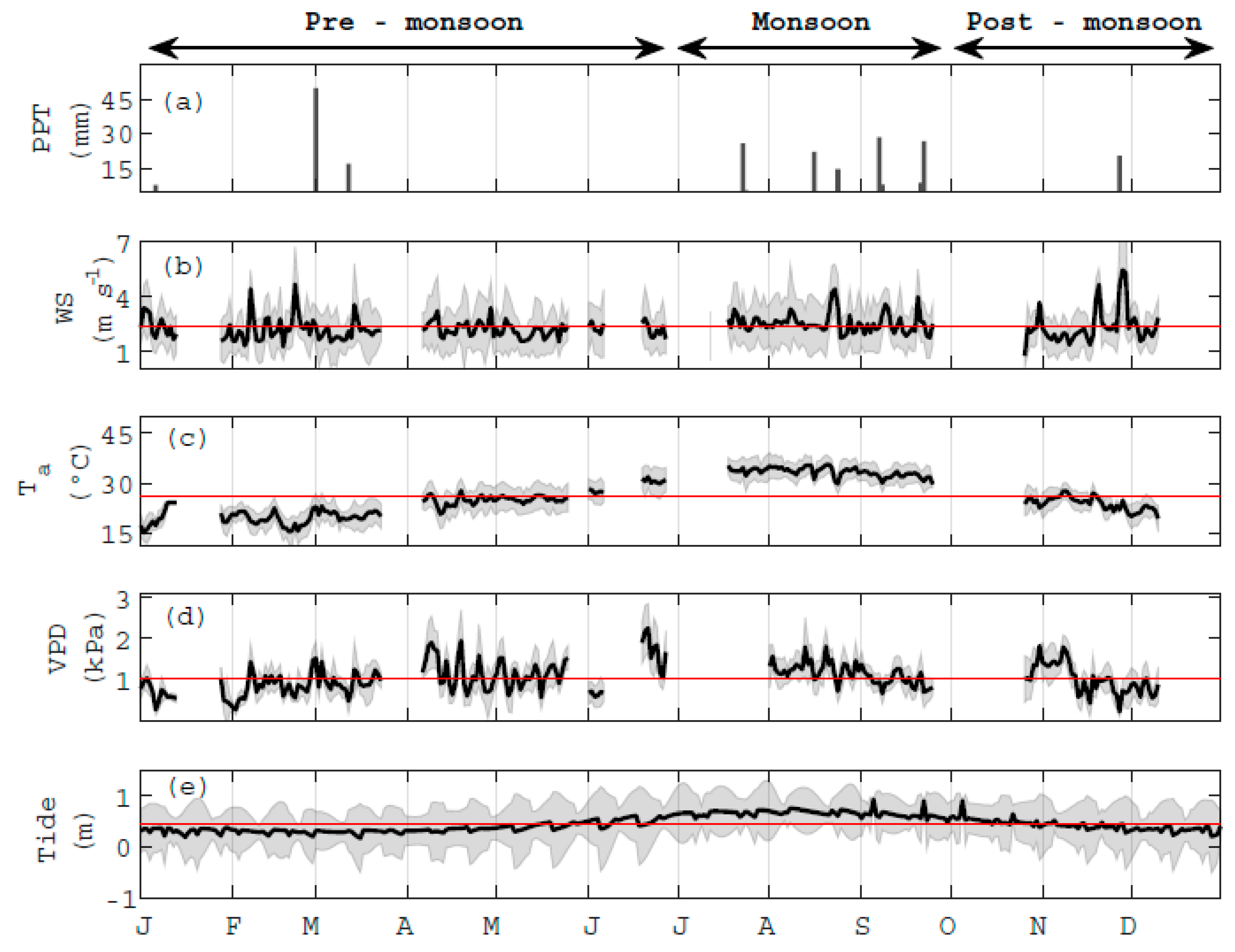
3.1. Micrometeorological Conditions

At this site in the Gulf of California, the patterns of wind direction and speed vary by season. During the transition season, defined here as the pre-monsoon, the direction from the continent to the ocean (N, NE) is more frequent from January to March; then, from April to June, the wind coming from the ocean (S, SW) increases in frequency (Figure 2a). This pattern of winds from the S and SW remains through all the monsoon season (Figure 2b). Then during the post-monsoon season (Figure 2c), there is an increase in continental winds from the N and NE. The observed wind patterns are typical of the region, were synoptic process such as the NAMS greatly influence climatic conditions.

In Figure 3, we observe the daily accumulated precipitation (mm), and daily averages of wind speed (WS, m s⁻¹), air temperature (T_a, °C), vapor pressure deficit (VPD, kPa) and tide height (m), as well as their variability from January to December 2019. Generally, T_a and VPD are lower during the first three months of the pre-monsoon season and the post-monsoon season, and higher during the monsoon season from July to October a typical pattern of this latitude (27° N).

During 2019, annual precipitation reached 258.9 mm, which is close to long-term annual observations for the region. Most of the observed precipitation events recordings were in the monsoon season (152.3 mm). However, some precipitation events occurred during the pre-monsoon season in January (7.62 mm), and March (66.4 mm), due to cold fronts. They also contributed to rainfall events in November (30.2 mm) (Figure 3a).

Based on the annual (2019) measurements, the average wind speed is 2.33 m s⁻¹ (Figure 3b); the range goes from 0.5 to 23 m s⁻¹ when maximum WS is considered (not shown in this figure). However, observations above 10 m s⁻¹ are not frequent at this site. Daily wind speed average during the pre-monsoon and the post-monsoon season was below the annual average and the during the monsoon season above it (Figure 3b).

We observed significant changes in air temperature (T_a) throughout the year; the range goes from 10 to 45 °C (Figure 3c). During the pre-monsoon T_a fluctuates from 10 to 37 °C; during the monsoon season it goes from 27 to 45 °C; then, during the post-monsoon season, it goes from 15 to 33 °C. During the pre-monsoon season, T_a fluctuates the most. The record of mean annual T_a was 25.9 °C. From July (Julian day 200) to September (Julian day 270), T_a was consistently above average, even during the night (Figure 3c). While during the other months, the T_a decreased below average.

VPD is highly variable as well (Figure 3d), and ranges from 0.055 kPa to 3.6 kPa; during the pre-monsoon season, we observe the lowest VPD on average in January (0.6 kPa) and again in December (0.8 kPa) during the post-monsoon, while, during the monsoon season (July-September), VPD increases to about the double especially in August (1.2 kPa). VPD annual mean is 1.023 kPa pre-monsoon, and post-monsoon VPD is below average, whereas during the monsoon, VPD is above average.

The tide in the region is characterized by a semi-diurnal cycle, adding to the dynamic regime of neap and spring tides. Furthermore, during the monsoon months, the water level in the coastal lagoon is above average, and the coastal system is always flooded (Figure 3e). During the pre-monsoon and post-monsoon, the water level is lower—in fact, in some sections of the coastal lagoon, the benthic zone will be exposed to the atmosphere. The channel in the inlet (Figure 1a) will have water all year round, and the minimum height is 0.4 m.

3.2. Monthly and Seasonal Variation of Meteorological Conditions, Turbulent Fluxes, and Energy Partitioning

Monthly average wind speed does not vary considerably throughout the year. WS was higher during August (2.6 m s⁻¹), July (2.5 m s⁻¹), and September (2.4 m s⁻¹). The lowest monthly average values occurred during March (2 m s⁻¹) and May (2 m s⁻¹). The monthly mean friction velocity (u*) variation was similar to WS. We observed the lowest values in January (0.18 m s⁻¹) and December (0.22 m s⁻¹) during the pre-monsoon and Post–monsoon season, respectively. Furthermore, higher u* records in April (0.27 m s⁻¹), May (0.27 m s⁻¹), and July (0.28 m s⁻¹) (

Table 1. Estero El Soldado coastal lagoon monthly average (and standard deviation in parentheses) of micrometeorological drivers and energy partitioning ratios. From left to right WS (wind speed), u* (friction velocity), VPD (vapor pressure deficit), Ta (air temperature), Tw (water temperature), H (sensible heat flux), LE (latent heat flux), and Rn (net radiation).

Month	Micrometeorological Drivers					Energy Partitioning
	WS (m/s)	u* (m/s)	VPD (kPa)	Ta (°C)	Tw (°C)	Albedo (α)	Bowen Ratio (β)	(H + LE)/Rn ratio
January	2.3 (1.27)	0.18 (0.09)	0.637 (0.329)	19.6 (4.0)	20.7 (3.1)	0.16 (0.01)	0.15	0.90
February	2.3 (1.41)	0.23 (0.14)	0.819 (0.383)	18.9 (3.8)	20.4 (3.4)	0.10 (0.00)	0.17	0.60
March	2.0 (1.32)	0.23 (0.13)	0.957 (0.415)	20.6 (3.7)	21.9 (2.6)	0.09 (0.00)	0.23	0.50
April	2.3 (1.42)	0.27 (0.16)	1.167 (0.635)	24.6 (4.2)	25.8 (3.0)	0.09 (0.00)	0.26	0.50
May	2.0 (1.19)	0.27 (0.17)	1.109 (0.463)	25.4 (6.5)	28.1(2.7)	0.10 (0.00)	0.37	0.60
June	2.2 (1.29)	0.25 (0.13)	1.259 (0.738)	29.3 (4.1)	30.3 (2.1)	0.09 (0.00)	0.26	0.30
July	2.5 (1.31)	0.28 (0.14)	-	33.9 (3.5)	30.6 (0.5)	0.03 (0.10)	-	-
August	2.6 (1.52)	0.26 (0.14)	1.268 (0.421)	33.9 (3.2)	32.8 (1.9)	0.08 (0.00)	0.20	0.70
September	2.4 (1.29)	0.24 (0.13)	0.974 (0.338)	32.2 (3.1)	30.5 (2.2)	0.09 (0.01)	0.18	0.80
October	2.1 (1.07)	0.23 (0.13)	1.166 (0.498)	24.9 (3.7)	25.0 (1.8)	0.12 (0.01)	0.16	0.40
November	2.4 (1.71)	0.25 (0.14)	1.021 (0.511)	24.4 (3.2)	23.3 (1.8)	0.12 (0.00)	0.08	0.80
December	2.2 (1.02)	0.22 (0.10)	0.783 (0.372)	21.6 (3.4)	19.8 (1.9)	0.18 (0.02)	0.23	0.40

).

As mentioned in the section above, VPD and T_a are highest during the monsoon season (Figure 3). The highest value recorded of VPD was in August (1267 Pa, Table 1); this was also the case for T_a (33.9 °C) and water temperature T_w (32.8 °C) (Table 1).

Estimates of average T_w are higher than T_a during the pre-monsoon months from January to June, and the post-monsoon months as well (Table 1). The reason for this is the diurnal variability; T_w does not vary as much as T_a during the night and day because of the heat storage capacity of water. Such diurnal variability, especially from T_a, is less prominent during the monsoon and warmest season of the year (Figure 3c).

The SW_in was significantly (p < 0.05) lower in December (69.6), and January (87.4), (Figure 4a). SW_in was highest in July (481.3), June (350.7), and May (349.8). During the pre-monsoon, SW_in was 257.8 ± 107.7 W m⁻², it was highest during the monsoon 313.11 ± 150.9 W m⁻², and lowest during the post-monsoon 132.7 ± 62.7 W m⁻². We observed a significant (p < 0.05) decrease from July to August, associated with cloud formation during the NAMS.

Net radiation (Rn) varies through the year, and we observe statistical differences (p < 0.05) at a monthly time scale. Rn was highest in June (493.8 W m⁻²), and July (407.2 W m⁻²), while lowest in January (92.3 W m⁻²), November (111.2 W m⁻²), September (177.3 W m⁻²), and February (188 W m⁻²) (Figure 4b). The average Rn during the pre-monsoon season was 275.2 W m⁻², barely lower than the monsoon season 276.8 W m⁻²; however, the standard deviation during the first was 137.3 W m⁻², while during the monsoon was 118 W m⁻², as a result of a month to month variability during the pre-monsoon the transition part of the year (Figure 4b).

Latent heat (LE) follows a similar trend to Rn, with high values in August (142.5 W m⁻²), May (138.9 W m⁻²), and April (135.9 W m⁻²). While, significantly lower values (p < 0.05) are in December (73.5 W m⁻²), and January (74.9 W m⁻²) (Figure 4c). LE is highest during the monsoon season 129.8 ± 17.9 W m⁻², followed by the pre-monsoon with 110.6 ± 2.6 W m⁻², and lastly, the post-monsoon season 94 ± 27.25 W m⁻². There is up to a 30% difference between the monsoon and post-monsoon season.

Consistently, sensible heat (H) is significantly (p < 0.05) lower in January (11.5 W m⁻²), February (15.5 W m⁻²), October (19.9 W m⁻²), November (6.3 W m⁻²), and December (17.0 W m⁻²) (Figure 4d). While H accounts only for about 10 % of annual Rn, its magnitude varies with season. During the pre-monsoon H was 28 ± 14.5 W m⁻², it was highest during the monsoon 29.4 ± 19.1 W m⁻², and lowest during the post-monsoon 14.4 ± 7.1 W m⁻².

Through this year-round study, LE and H are always positive fluxes, transporting energy from the water surface to the atmosphere. The amount of Rn influences the magnitude of these turbulent fluxes in the system. Furthermore, the energy partitioning through the albedo (α), Bowen (β), and (H + LE)/Rn ratios are a good insight on how much absorbed radiation there is, and how energy is used.

Albedo from ocean surfaces without ice is low ~0.08 [6]; therefore, most of the incoming solar radiation is absorbed. In this semiarid coastal lagoon, the seasonal average of albedo was lower in the monsoon (0.07), with the lowest monthly mean value in July (0.03) (Table 1). During January, February, November, and December (Figure 3e and Table 1), months from the pre-monsoon and post-monsoon seasons, albedo increases by about ~9%. At the same zenith angle (20 to 40°) from 10 to 15 h, albedo is lower (0.09) with a higher water column (>0.45 m) than when the water column is lower (<0.45 m) as, in this case, the average albedo increases (0.11). A shorter water column influences albedo via interactions with the clear sandy sediment and water transparency [52]. Furthermore, ocean surface albedo can be sensitive to zenith angle and wind speed [53], at this site during the same zenith angle (20° to 40°), the albedo was 0.05 either at low WS conditions (<2.03 m s⁻¹) or high wind conditions (>9 m s⁻¹). Finally, during the monsoon season, we observe that albedo during the same zenith angle (20 to 40°) is higher through cloudy days (0.11) than clear-sky days (0.07). Further research should explore these interactions at different zenith angles and wind speeds.

As expected, the Bowen ratio (β) is highest during the pre-monsoon (0.24) and lowest during the post-monsoon (0.16) season (Table 1). The reduced magnitude of β is the result of the lower values of H. The lowest monthly mean β value was during the post-monsoon season in November (0.08), and the highest was during the pre-monsoon season in May (0.37) (Table 1).

On the other hand, the ratio of turbulent fluxes to net radiation (H + LE)/Rn also changed with seasons. During the monsoon, the highest seasonal ratio (0.74) was observed, with the highest monthly mean in September (0.80) (Table 1). The lowest observations recorded were during the post-monsoon (0.54), with December and October being the lowest (0.40). Although the pre-monsoon season average was not the highest (0.58), during January, (H + LE)/Rn ratio value was 0.90. In terms of energy exchange, the annual average of (H + LE)/Rn ratio (0.59) suggests that about half of the Rn reaching the EES coastal lagoon through the year transforms in a turbulent exchange of H and LE. Seasonally, pre-monsoon (H + LE)/Rn ratio suggests that the surface uses only a little more than half of Rn. In contrast, more than half the amount of Rn during the monsoon season (0.74) goes to turbulent fluxes. The fact that there is a higher ratio during the pre-monsoon than during the post-monsoon season relates to energy stored in the water due to heat capacity, that further transfers between season [36,54].

In context with other sites, Rn at higher latitudes is lower than at this coastal lagoon in the Gulf of California (Table 1). In comparison, Rn is about 48% more, LE flux is 40% more, and H flux is 50% more at any given time of the year. With some exceptions, like in Lake W (Canada) during the monsoon, where LE was 44 W m⁻² higher than at EES. The higher amount of LE at Lake W links to low solar radiation and a negative flux of H in the bottom of the lake [32]. This phenomenon does not occur at the shallow, and tide-influenced EES. The other exception was the H flux in Ross Barnett Reservoir (USA) [16]; during the post-monsoon, H was about double than in EES (

Table 2. Net radiation (Rn), latent heat (LE), and sensible heat (H) from water bodies at different latitudes. Data were organized based on seasons in this study, were pre-monsoon (January–June), monsoon (July–September), and post-monsoon (October-December).

Season	Rn	LE	H	Site	Latitude	Author
	(W m−2)	(W m−2)	(W m−2)
Pre-monsoon
	117.83	77.46	15.06	Ross Barnett Reservoir, USA	32° N	[16]
	275.2	110	28	Estero El Soldado, Mexico	27° N	This study
Monsoon
	165	173	−23	Lake W, Canada	58° N	[32]
	148.5	118.46	15.36	Ross Barnett Reservoir, USA	32° N	[16]
	146.84	79.74	22.35	Lake Ngoring, China	35° N	[36]
	276.8	129	29	Estero El Soldado, Mexico	27° N	This study
Post-monsoon
	49.16	74.9	22.9	Ross Barnett Reservoir, USA	32° N	[16]
	234.7	94	14	Estero El Soldado, Mexico	27° N	This study

).

3.3. Diurnal Variations of R_n and Turbulent Fluxes

In general, all three fluxes Rn, LE, H, increase at 6 h, reaching a maximum at noon, and decreasing around 19 h (Figure 5). During the pre-monsoon season, the average values of Rn are similar of those from the monsoon season; however, the variability is much higher during the pre-monsoon season (Figure 5a). Rn during the monsoon drops around noon (Figure 5b), associated with convective clouds, which are more frequent during the NAMS.

From 10 to 13 h, during the pre-monsoon season, there is up to 20% more Rn than in the monsoon and post-monsoon. While at this same time period, LE is 20% more during the monsoon than the pre-monsoon and up to 40% more than in the post-monsoon season. Finally, during the post-monsoon season there is 38% less H flux available, than in the pre-monsoon and monsoon seasons.

It is clear that, with more Rn available in this coastal system, there is an increase in LE and H. Studies focused on better understanding turbulent fluxes over water have reported that the LE always prevails over H, whether is a semiarid [21,22], or a temperate region [55,56]. In this study, we observe how LE consumes almost 40 % of Rn (Table 2 and Figure 5), for all three seasons. The fact that this coastal lagoon is located in the mid-region of the Gulf of California, and therefore influenced by the North American Monsoon System [40], is especially noticeable when analyzing the Rn and SW_in.

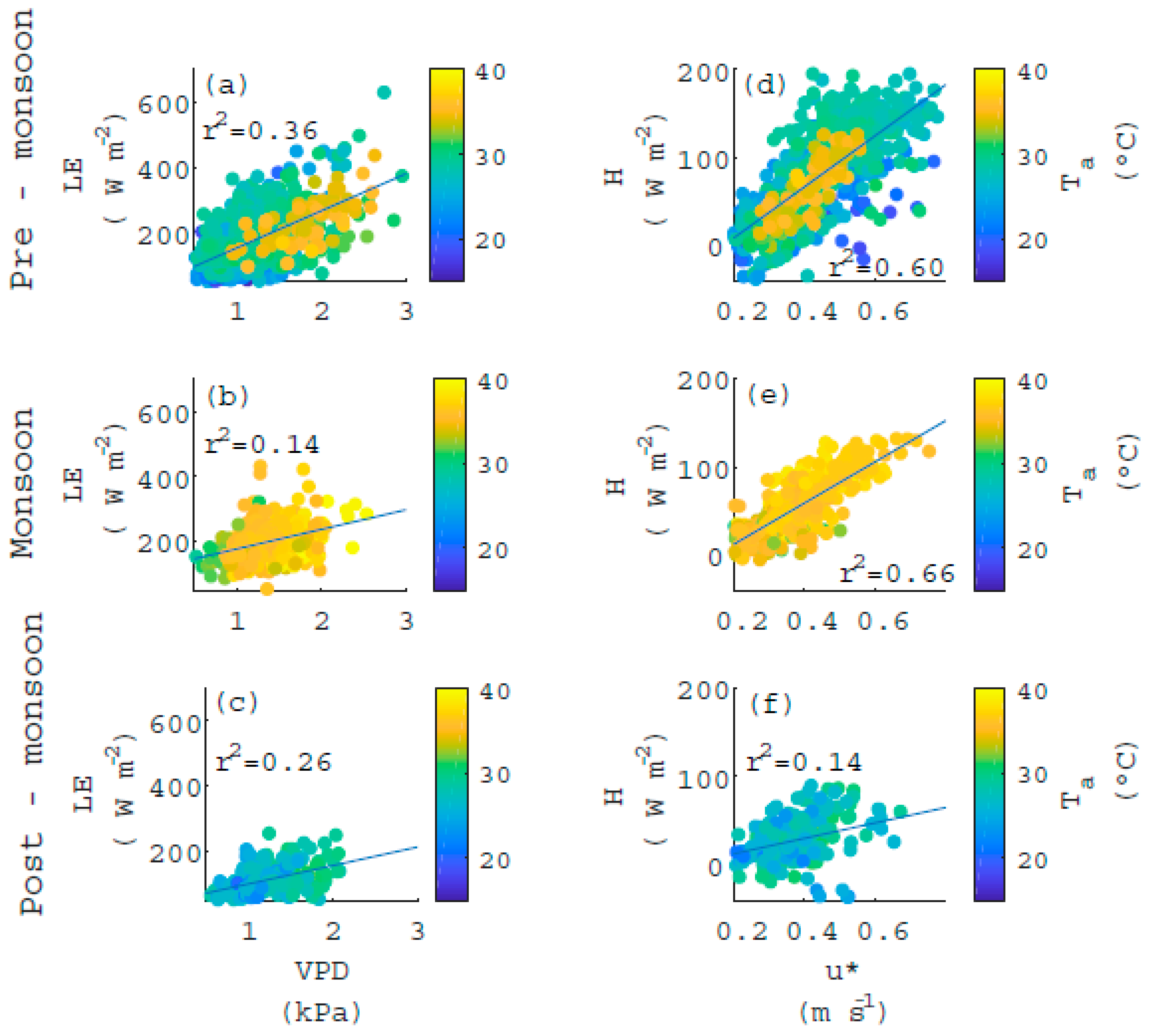
3.4. Micrometeorological Drivers and Turbulent Fluxes

We analyzed the correlation during the pre-monsoon, monsoon, and post-monsoon of vapor pressure deficit (VPD) and latent heat (LE); and friction velocity (u*) and sensible heat (H), using data from 10 to 15 h (zenith angle 20° to 40°).

During the pre-monsoon season, as VPD increases, the turbulent flux of LE increases (r² = 0.36) from 50 to 250 W m⁻², in particular from 0.5 kPa to 1.5 kPa at T_a of around 25–30 °C (Figure 6a). In this same season (Figure 6d) as u* ranges from 0.3 to 0.45 m s⁻¹, H flux increases (r² = 0.60) from 20 to 80 W m⁻² with T_a between 25–30 °C.

During the monsoon, as VPD increases from 1 kPa to 1.8 kPa, the LE flux increases as well (r² = 0.14) from 100 to 300 W m⁻² at T_a around 35–40 °C (Figure 6b). Furthermore, when u* increases from 0.2 to 0.6 m s⁻¹, H flux increases (r² = 0.66) from 20 to 120 W m⁻² at T_a between 35–40 °C, this is the best correlation for H flux from each season analyzed here (Figure 6e).

Through the post-monsoon season, VPD ranges between 0.5 kPa and 1.5 kPa similar to the pre-monsoon season, and the LE flux (r² = 0.26) goes from 60 to 120 W m⁻² with a T_a around 25 °C (Figure 6c). Similarly, to previous seasons, as u* increases from 0.3 to 0.45 m s⁻¹, there is an increase in the H flux (r² = 0.14) of −20 to 80 at T_a around 25 °C (Figure 6f), this correlation, however, is not very strong.

Turbulent fluxes are sensitive to air temperature (T_a), vapor pressure deficit (VPD), and friction velocity (u*), as previously observed in other studies [4,17,22,57]. Interestingly, while H increases with higher u* and high T_a during the monsoon season, LE does not increase as much with higher atmospheric demand during this same period. During the pre-monsoon season, however, VPD can better explain the change in LE flux, especially at higher T_a (Figure 6). Overall, the sensitivity of turbulent fluxes to micrometeorological conditions changes with the season at this semiarid coastal lagoon. While H flux is more sensitive during the pre-monsoon and monsoon, LE is more sensitive during the pre-monsoon.

4. Summary and Conclusions

The present study provides observations of Rn, LE, and H flux and its variability at diurnal, monthly, and season scales for an annual period (2019), from a coastal lagoon. The aim of this study was to better understand the turbulent fluxes between the surface water and the air. A limitation of this study, however, is the lack of information on the energy stored in the water column. Despite this limitation, we believe reporting on the Rn and turbulent fluxes of LE and H is important for the atmospheric science, hidrometerology, ecohydrology, and the modeling community. This study is the first to assess Rn, and turbulent fluxes of LE and H in a coastal lagoon of the Gulf of California.

At this coastal lagoon the wind direction after the monsoon season is from the continent to the ocean (N, NE), and it changes towards the continent from the ocean (S, SW) from Abril and through the monsoon season. This air provides moist for cloud formation, SW_in and Rn decreased especially in August due to this phenomenon. However, Rn, LE, and H were higher during the monsoon season than any other season. Albedo at this site changes with water column height but not with wind speed at same zenith angle, further research is needed to better understand this dynamic.

The Rn at this site is 40% higher than at other mid-latitudes. Furthermore, LE correlates to VPD during the pre-monsoon and H correlates with u* during the monsoon season.

References

1. Garstang, M. Sensible and latent heat exchange in low latitude synoptic scale systems. Tellus 1967, 19, 492–508. [Google Scholar] [CrossRef] [Green Version]
2. Stannard, D.; Gannett, M.; Polette, D.; Cameron, J.; Waibel, M.; Spears, J. Evaporation from Marsh and Open-Water Sites at Upper Klamath Lake, Oregon, 2008–2010; U.S. Geological Survey: Reston, VA, USA, 2013; p. 66.
3. Stull, R. An Introduction to Boundary Layer Meteorology; Kluwer Acad. Publ.: Boston, MA, USA; London, UK, 1988; p. 666. [Google Scholar]
4. Nordbo, A.; Launiainen, S.; Mammarella, I.; Leppäranta, M.; Huotari, J.; Ojala, A.; Vesala, T. Long-term energy flux measurements and energy balance over a small boreal lake using eddy covariance technique. J. Geophys. Res. Atmos. 2011, 116, 1–17. [Google Scholar] [CrossRef]
5. Smith, N.P. Local energy exchanges in a shallow, coastal lagoon: Summer conditions. Atmos. Ocean 1981, 19, 307–319. [Google Scholar] [CrossRef]
6. Shuttleworth, W. Terrestrial Hydrometeorology; Wiley-Blackwell: Oxford, UK, 2012; p. 441. [Google Scholar]
7. Wallace, J.M.; Hobbs, P.V. Atmospheric Science: An. Introductory Survey; Academic Press: Cambridge, MA, USA, 2006; p. 483. [Google Scholar]
8. Smith, S.V.; Atkinson, M.J. Mass balance of nutrient fluxes in coastal lagoons. In Elsevier Oceanography Series; Elsevier: Amsterdam, The Nethrelands, 1994; pp. 133–155. [Google Scholar]
9. Smith, N.P. Water, salt and heat balance of coastal lagoons. In Elsevier Oceanographic Series; Elsevier: Amsterdam, The Netherlands, 1994; Volume 60. [Google Scholar]
10. Talley, L.; Pickard, G.; Emery, W.; Swift, J. Chapter 5—Mass, Salt, and Heat Budgets and Wind Forcing. In Descriptive Physical Oceanography: An Introduction; Academic Press: Cambridge, MA, USA, 2011. [Google Scholar]
11. Duan, Z.; Bastiaanssen, W. A new empirical procedure for estimating intra-annual heat storage changes in lakes and reservoirs: Review and analysis of 22 lakes. Remote Sens. Environ. 2015, 156, 143–156. [Google Scholar] [CrossRef]
12. Zhang, Y.; Perrie, W. Feedback mechanisms for the atmosphere and ocean surface. Bound.-Layer Meteorol. 2001, 100, 321–348. [Google Scholar] [CrossRef]
13. Martínez-Alvarez, V.; Gallego-Elvira, B.; Maestre-Valero, J.; Tanguy, M. Simultaneous solution for water, heat and salt balances in a Mediterranean coastal lagoon (Mar Menor, Spain). Estuar. Coast. Shelf Sci. 2011, 91, 250–261. [Google Scholar] [CrossRef]
14. Hostetler, S.; Bartlein, P. Simulation of lake evaporation with application to modeling lake level variations of Harney-Malheur Lake, Oregon. Water Resour. Res. 1990, 26, 2603–2612. [Google Scholar]
15. Blanken, P.D.; Rouse, W.R.; Schertzer, W.M. Enhancement of evaporation from a large northern lake by the entrainment of warm, dry air. J. Hydrometeorol. 2003, 4, 680–693. [Google Scholar] [CrossRef] [Green Version]
16. Liu, H.; Zhang, Q.; Dowler, G. Environmental controls on the surface energy budget over a large southern inland water in the United States: An analysis of one-year eddy covariance flux data. J. Hydrometeorol. 2012, 13, 1893–1910. [Google Scholar] [CrossRef]
17. Shao, C.; Chen, J.; Stepien, C.A.; Chu, H.; Ouyang, Z.; Bridgeman, T.B.; Czajkowski, K.P.; Becker, R.H.; John, R. Diurnal to annual changes in latent, sensible heat, and CO2 fluxes over a Laurentian Great Lake: A case study in Western Lake Erie. J. Geophys. Res. Biogeosci. 2015, 120, 1587–1604. [Google Scholar] [CrossRef]
18. Walker, A.S. Deserts: Geology and Resources; US Department of the Interior, US Geological Survey: Reston, VA, USA, 2000.
19. Noy-Meir, I. Desert ecosystems: Environment and producers. Annu. Rev. Ecol. Syst. 1973, 4, 25–51. [Google Scholar] [CrossRef]
20. Ali, S.; Ghosh, N.C.; Singh, R. Evaluating best evaporation estimate model for water surface evaporation in semi-arid region, India. Hydrol. Process. Int. J. 2008, 22, 1093–1106. [Google Scholar] [CrossRef]
21. Sánchez-Carrillo, S.; Angeler, D.G.; Sánchez-Andrés, R.; Alvarez-Cobelas, M.; Garatuza-Payán, J. Evapotranspiration in semi-arid wetlands: Relationships between inundation and the macrophyte-cover: Open-water ratio. Adv. Water Resour. 2004, 27, 643–655. [Google Scholar] [CrossRef]
22. Sun, J.; Hu, W.; Zhao, L.; An, R.; Ning, K.; Zhang, X. Eddy covariance measurements of water vapor and energy flux over a lake in the Badain Jaran Desert, China. J. Arid Land 2018, 10, 517–533. [Google Scholar] [CrossRef] [Green Version]
23. Adams, D.K.; Comrie, A.C. The north American monsoon. Bull. Am. Meteorol. Soc. 1997, 78, 2197–2214. [Google Scholar] [CrossRef] [Green Version]
24. Bohn, T.J.; Vivoni, E.R. Process-based characterization of evapotranspiration sources over the North American monsoon region. Water Resour. Res. 2016, 52, 358–384. [Google Scholar] [CrossRef] [Green Version]
25. Barlow, M.; Nigam, S.; Berbery, E.H. Evolution of the North American monsoon system. J. Clim. 1998, 11, 2238–2257. [Google Scholar] [CrossRef]
26. McGowan, H.; Sturman, A.; Saunders, M.; Theobald, A.; Wiebe, A. Insights from a decade of research on coral reef—Atmosphere energetics. J. Geophys. Res. Atmos. 2019, 124, 4269–4282. [Google Scholar] [CrossRef]
27. Jung, M.; Reichstein, M.; Margolis, H.A.; Cescatti, A.; Richardson, A.D.; Arain, M.A.; Arneth, A.; Bernhofer, C.; Bonal, D.; Chen, J. Global patterns of land-atmosphere fluxes of carbon dioxide, latent heat, and sensible heat derived from eddy covariance, satellite, and meteorological observations. J. Geophys. Res. Biogeosci. 2011, 116, G00J07. [Google Scholar] [CrossRef] [Green Version]
28. Baldocchi, D.; Falge, E.; Gu, L.; Olson, R.; Hollinger, D.; Running, S.; Anthoni, P.; Bernhofer, C.; Davis, K.; Evans, R.; et al. FLUXNET: A new tool to study the temporal and spatial variability of ecosystem-scale carbon dioxide, water vapor, and energy flux densities. Bull. Am. Meteorol. Soc. 2001, 82, 2415–2434. [Google Scholar] [CrossRef]
29. Baldocchi, D. Measuring fluxes of trace gases and energy between ecosystems and the atmosphere—The state and future of the eddy covariance method. Glob. Chang. Biol. 2014, 20, 3600–3609. [Google Scholar] [CrossRef] [PubMed]
30. Su, Z. The Surface Energy Balance System (SEBS) for estimation of turbulent heat fluxes. Hydrol. Earth Syst. Sci. 2002, 6, 85–99. [Google Scholar] [CrossRef]
31. Aubinet, M.; Vesala, T.; Papale, D. Eddy Covariance: A practical Guide to Measurement and Data Analysis; Springer: Berlin/Heidelberg, Germany, 2012. [Google Scholar]
32. Bello, R.; Smith, J. The effect of weather variability on the energy balance of a lake in the Hudson Bay Lowlands, Canada. Arct. Alp. Res. 1990, 22, 98–107. [Google Scholar] [CrossRef]
33. Blanken, P.D.; Rouse, W.R.; Culf, A.D.; Spence, C.; Boudreau, L.D.; Jasper, J.N.; Kochtubajda, B.; Schertzer, W.M.; Marsh, P.; Verseghy, D. Eddy covariance measurements of evaporation from Great Slave lake, Northwest Territories, Canada. Water Resour. Res. 2000, 36, 1069–1077. [Google Scholar] [CrossRef]
34. Rouse, W.R.; Blanken, P.D.; Bussières, N.; Walker, A.E.; Oswald, C.J.; Schertzer, W.M.; Spence, C. An investigation of the thermal and energy balance regimes of Great Slave and Great Bear Lakes. J. Hydrometeorol. 2008, 9, 1318–1333. [Google Scholar] [CrossRef]
35. Hutjes, R.; Kabat, P.; Running, S.; Shuttleworth, W.; Field, C.; Bass, B.; Dias, M.; Avissar, R.; Becker, A.; Claussen, M.; et al. Biospheric aspects of the hydrological cycle—Preface. J. Hydrol. 1998, 212, 1–2. [Google Scholar] [CrossRef]
36. Li, Z.; Lyu, S.; Ao, Y.; Wen, L.; Zhao, L.; Wang, S. Long-term energy flux and radiation balance observations over Lake Ngoring, Tibetan Plateau. Atmos. Res. 2015, 155, 13–25. [Google Scholar] [CrossRef]
37. Sonora, G. Programa de manejo de la zona sujeta a conservación ecológica estero el soldado Cedeyd. Sustentable; Gobierno del Estado de Sonora: Sonora, Mexico, 2018. [Google Scholar]
38. Filloux, J. Tidal patterns and energy balance in the Gulf of California. Nature 1973, 243, 217. [Google Scholar] [CrossRef]
39. García, E. Modificaciones al Sistema de Clasificación Climática de Köppen (para adaptarlo a las condiciones de la República Mexicana), 5th ed.; México, D.F., Ed.; Offset Larios: Larios, Mexico, 1988. [Google Scholar]
40. Gochis, D.; Brito-Castillo, L.; Shuttleworth, W. Hydroclimatology of the North American Monsoon region in northwest Mexico. J. Hydrol. 2006, 316, 53–70. [Google Scholar] [CrossRef]
41. Nakai, T.; van der Molen, M.; Gash, J.; Kodama, Y. Correction of sonic anemometer angle of attack errors. Agric. For. Meteorol. 2006, 136, 19–30. [Google Scholar] [CrossRef] [Green Version]
42. Wilczak, J.M.; Oncley, S.P.; Stage, S.A. Sonic anemometer tilt correction algorithms. Bound.-Layer Meteorol. 2001, 99, 127–150. [Google Scholar] [CrossRef]
43. Runkle, B.R.; Wille, C.; Gažovič, M.; Kutzbach, L. Attenuation correction procedures for water vapour fluxes from closed-path eddy-covariance systems. Bound. Layer Meteorol. 2012, 142, 401–423. [Google Scholar] [CrossRef]
44. Webb, E.K.; Pearman, G.I.; Leuning, R. Correction of flux measurements for density effects due to heat and water vapour transfer. Q. J. R. Meteorol. Soc. 1980, 106, 85–100. [Google Scholar] [CrossRef]
45. Horst, T. A simple formula for attenuation of eddy fluxes measured with first-order-response scalar sensors. Bound.-Layer Meteorol. 1997, 82, 219–233. [Google Scholar] [CrossRef]
46. Vickers, D.; Mahrt, L. Quality control and flux sampling problems for tower and aircraft data. J. Atmos. Ocean. Technol. 1997, 14, 512–526. [Google Scholar] [CrossRef]
47. Mauder, M. A Comment on “How Well Can We Measure the Vertical Wind Speed? Implications for Fluxes of Energy and Mass” by Kochendorfer et al. Bound.-Layer Meteorol. 2013, 147, 329–335. [Google Scholar] [CrossRef]
48. Kljun, N.; Calanca, P.; Rotach, M.; Schmid, H. A simple two-dimensional parameterisation for Flux Footprint Prediction (FFP). Geosci. Model. Dev. 2015, 8, 3695. [Google Scholar] [CrossRef] [Green Version]
49. Mauder, M.; Liebethal, C.; Gockede, M.; Leps, J.P.; Beyrich, F.; Foken, T. Processing and quality control of flux data during LITFASS-2003. Bound. Layer Meteorol. 2006, 121, 67–88. [Google Scholar] [CrossRef]
50. Wilson, K.; Goldstein, A.; Falge, E.; Aubinet, M.; Baldocchi, D.; Berbigier, P.; Bernhofer, C.; Ceulemans, R.; Dolman, H.; Field, C. Energy balance closure at FLUXNET sites. Agric. For. Meteorol. 2002, 113, 223–243. [Google Scholar] [CrossRef] [Green Version]
51. Kidston, J.; Brümmer, C.; Black, T.A.; Morgenstern, K.; Nesic, Z.; McCaughey, J.H.; Barr, A.G. Energy balance closure using eddy covariance above two different land surfaces and implications for CO2 flux measurements. Bound. Layer Meteorol. 2010, 136, 193–218. [Google Scholar] [CrossRef]
52. Jin, Z.; Charlock, T.P.; Smith, W.L., Jr.; Rutledge, K. A parameterization of ocean surface albedo. Geophys. Res. Lett. 2004, 31, 1195636. [Google Scholar] [CrossRef]
53. Nunez, M.; Davies, J.; Robinson, P. Surface albedo at a tower site in Lake Ontario. Bound.-Layer Meteorol. 1972, 3, 77–86. [Google Scholar] [CrossRef]
54. Smith, N.P. Energy balance in a shallow seagrass flat for winter conditions 1. Limnol. Oceanogr. 1981, 26, 482–491. [Google Scholar] [CrossRef]
55. Souch, C.; Grimmond, S.; Wolfe, C. Evapotranspiration rates from wetlands with different disturbance histories: Indiana Dunes National Lakeshore. Wetlands 1998, 18, 216–229. [Google Scholar]
56. Vesala, T.; Huotari, J.; Rannik, Ü.; Suni, T.; Smolander, S.; Sogachev, A.; Launiainen, S.; Ojala, A. Eddy covariance measurements of carbon exchange and latent and sensible heat fluxes over a boreal lake for a full open-water period. J. Geophys. Res. Atmos. 2006, 111, D11101. [Google Scholar] [CrossRef]
57. Bouin, M.N.; Caniaux, G.; Traullé, O.; Legain, D.; le Moigne, P. Long-term heat exchanges over a Mediterranean lagoon. J. Geophys. Res. Atmos. 2012, 117, D23104. [Google Scholar] [CrossRef]
Figure 1. The study site is located in the inlet of a coastal lagoon (a), in the Gulf of California northwestern México (b). In (c), the triangle represents the exact location (27°57.248′ N, 110°58.350′ W), contour lines represent the frequency of the climatological footprint, and (d) shows the monitoring system.
Atmosphere 11 00626 g001
Figure 2. The wind rose for the three studied seasons (a) pre-monsoon, (b) monsoon, and (c) post-monsoon. In panel (a) probability density function (PDF) from January (J) to March (M)—thin black line, and from April (A) to June (J)—thick gray line.
Atmosphere 11 00626 g002
Figure 3. Daily times series of (a) daily accumulated precipitation (PPT), in subsequent panels, daily average (black lines), standard deviation (grey shaded area), and annual mean (red line) of (b) wind speed (WS), (c) air temperature (Ta), (d) vapor pressure deficit (VPD), and (e) tide height. Initial in x-axis from left to right J (January), F (February), M (March), A (April), M (May), J (June), J (July), A (August), S (September), O (October), N (November), and D ( December).Data gaps originated from instrument failure, maintenance, or quality assurance and quality control (QA/QC).
Atmosphere 11 00626 g003
Figure 4. Monthly mean and standard deviation of (a) incoming solar radiation (SWin), (b) net radiation (Rn), (c) latent heat (LE), and (d) sensible heat (H) from January to December 2019. Initial in x-axis from left to right J (January), F (February), M (March), A (April), M (May), J (June), J (July), A (August), S (September), O (October), N (November), and D (December).
Atmosphere 11 00626 g004
Figure 5. Diurnal cycle average and standard deviation (shaded area), for net radiation (Rn), latent heat (LE), and sensible heat (H) fluxes during the (a) pre-monsoon (January–June), (b) monsoon (July–August), and (c) post-monsoon (September–December).
Atmosphere 11 00626 g005
Figure 6. Ordinary linear regression of turbulent fluxes and micrometeorological variables: correlation of vapor pressure deficit (VPD, kPa) with latent heat (LE, W m−2), and friction velocity (u*, m s−1) with sensible heat (H, W m−2), considering air temperature Ta, and seasonality: pre-monsoon (ad), monsoon (be), post-monsoon (cf). Data from 10 to 15 h were used.
Atmosphere 11 00626 g006