Abstract
A majority of the existing atmospheric rivers (ARs) detection methods is based on magnitude thresholding on either the integrated water vapor (IWV) or integrated vapor transport (IVT). One disadvantage of such an approach is that the predetermined threshold does not have the flexibility to adjust to the fast changing conditions where ARs are embedded. To address this issue, a new AR detection method is derived from an image-processing algorithm that makes the detection independent of AR magnitude. In this study, we compare the North Pacific and Atlantic ARs tracked by the new detection method and two widely used magnitude thresholding methods in the present day climate. The results show considerable sensitivities of the detected AR number, shape, intensities and their accounted IVT accumulations to different methods. In many aspects, ARs detected by the new method lie between those from the two magnitude thresholding methods, but stand out with a greater number of AR tracks, longer track durations, and stronger AR-related moisture transport in the AR tracks. North Pacific and North Atlantic ARs identified by the new method account for around 100–120 kg/m/s IVT within the AR track regions, about more than the other two methods. This is primarily due to the fact that the new method captures the strong IVT signals more effectively.
1. Introduction
An atmospheric river (AR) is often characterized as a narrow and elongated filament of enhanced water vapor content in the lower troposphere, within the warm conveyor belt of extratropical cyclones (e.g., [,,,]). A typical AR can carry 7–15 times the water in the Mississippi River [], and at any time in winter, there are three to five ARs in the Northern Hemisphere alone [], constituting the majority of meridional fluxes with about 10% of the zonal extent of the Earth [].
Most of the existing automated AR detection methods apply some kinds of thresholds on the integrated vapor transport (IVT) and/or integrated water vapor (IWV) distributions to achieve the detection. For instance, [] introduced the 2 cm IWV threshold and a 2000 km length requirement that have been followed by many ensuing studies (e.g., [,,]). A 250 kg/m/s IVT threshold was used by [,] to detect landfalling ARs onto the North America continent. Although easy to interpret and implement, a globally applied constant threshold may become problematic when the underlying IVT and/or IWV distributions experience some low-frequency variations, or when applied to model simulations that come with different levels of biases. The alternative relative magnitude threshold, for instance, the 85th percentile of local climatology used in some studies (e.g., [,,]), offers greater flexibility to the basin, seasonal and latitudinal variations. However, it requires a large dataset to compute the percentile values, therefore may not have the flexibility to adopt to the fast-changing synoptic conditions where ARs are embedded.
To address the above problems, we recently developed a new AR detection method based on an image-processing technique—the top-hat by reconstruction (THR) algorithm []. The new approach exploits the transient nature of ARs, and achieves the detection by isolating moisture plumes that stand out from the typical spatio-temporal extent of synoptic systems. It is shown to have lower sensitivity to parameters and a greater tolerance to a wider range of water vapor flux intensities. This enhanced adaptability to varying AR intensities can help detecting the genesis or dissipating stages of some strong ARs, or some weaker but still sizable systems that do not meet the requirement of a prescribed IVT magnitude. More technical details of the new method are described in a separate submitted paper, in this work we focus on comparing some characteristics of the ARs tracked by the new THR method and two conventional magnitude thresholding methods: IVT250ano and IVT85%. The former uses a prescribed 250 kg/m/s threshold on the IVT anomalies, and the latter applies an IVT threshold primarily based on the local 85th percentile.
Methodological differences have been found to contribute considerably to the uncertainties in many AR-related statistics. For instance, the Atmospheric River Tracking Method Intercomparison Project (ARTMIP) [] complied eight different AR detection methods (some come with sub-catalogues with varying parameters) and applied them to the same Reanalysis dataset at a prescribed landfall region. The number of AR events for the period of 2005–2016 ranges from 131 to 268. The complex interactions of AR and terrain add extra sensitivity to the detection results. However, even over the open oceans, AR occurrence frequency is sensitive to the choice of the IVT threshold []. On the other hand, method-induced uncertainty problem is not unique to ARs. For extratropical cyclones that show close physical correspondences with ARs, considerable methodological discrepancies have been identified by the Intercomparison of Midlatitude Storm Diagnostics (IMILAST) project []. Similar to the case of ARs, greater uncertainty was found among cyclone tracks that are shorter-lived and weaker in intensity. These highlight the importance of a contextual understanding of the degree of uncertainties caused by detection methods in helping derive meaningful scientific interpretations from various statistics.
The focus of this study is on comparisons of ARs detected from IVT by the new THR method and by two widely used magnitude thresholding methods. Details of the methods are given in Section 2. The detected Northern Hemisphere wintertime ARs from different methods are compared in Section 3, covering the AR numbers, sizes and shapes, life cycles and seasonal IVT accumulations. Lastly, Section 4 summarizes the results and gives some concluding remarks.
2. Data and Methods
2.1. IVT and Precipitation Data
The vertically integrated horizontal moisture fluxes (, ) are obtained from the ECMWF’s ERA-I reanalysis product [] (https://www.ecmwf.int/en/forecasts/datasets/reanalysis-datasets/era-interim). IVT is computed as . The data have a horizontal resolution of and a temporal resolution of 6-h. The 6-hourly precipitation rates from ERA-I are also obtained. Previous studies have shown that the choice of the reanalysis dataset does not contribute much to the detection uncertainties [,]. Only the November–April seasons of the November 2004 to April 2010 period are used. As this study is mainly focused on the differences in the seasonal average statistics arising from different methods, these six winter seasons, providing a total of over 6000 AR occurrences, should serve a sufficient sample size.
2.2. Brief Introduction of the Image-Processing Based THR AR Detection Method
We took the inspiration from an existing image-processing technique, the top-hat by reconstruction (THR) algorithm [], and modified it into an AR detection method. More technical details of the algorithm are provided in a separate work, and the implementation in the Python programming language is posted at https://github.com/ihesp/IPART/releases/tag/v1.0. The detection process consists of the following basic steps:
- at each grid cell in the IVT data, perform a search for the minimum IVT value within a given neighborhood, which covers the region around that grid cell with a radius of ∼500 km in space, and 4 days in time—a characteristic spatio-temporal scale that corresponds to the physical processes of ARs.
- spread the found minimum values laterally and incrementally, subject to that they do not exceed the original IVT. After convergence, this step creates local plateaus with various heights.
- subtract from the original IVT distribution the results from step 2, giving the anomalous IVT component.
- in the anomalous IVT component, select contiguous regions where the anomalies are above zero. This marks out a collection of regions, those of which that pass the geometrical filtering are defined as ARs.
It is important to note that no threshold is imposed on AR magnitudes in this method. Instead, identification of an AR is based on its spatio-temporal “spikiness”, which is a key to distinguish this new method from the existing magnitude thresholding methods. Sensitivity tests revealed that detection number shows reduced sensitivity to the spatial and temporal radii parameters in the THR method compared to the sensitivity to the magnitude threshold in magnitude thresholding methods described below. Further details of the sensitivity analyses are given in the technical paper.
Then some geometrical filtering is applied on the above found AR candidates:
- length and area: the length of an AR is defined as the line integral of the AR axis, introduced in the following section. The length is required to be within 2000–11,000 km, and the region area is required to be 500 –10,000 km, to screen out features that are either too small or too large to conform to the definition of AR.
- isoperimetric quotient: defined as the ratio of the area enclosed by an AR candidate’s boundary and that of the circle having the same perimeter of the AR. More circular features (such as tropical cyclones) having isoperimetric quotients greater than are filtered out. Passing candidates are further filtered by a minimal length/width ratio of 2, where the width is defined as the ratio of area over length.
- latitudinal range: the geometrical centroid of an AR is required to be within 23–80, to select only mid-latitude systems.
After geometrical filtering, passing candidates are regarded as ARs. The spatial region an AR occupies is termed the “AR region”, and the appearance at an instantaneous time point an “AR occurrence”.
2.3. AR Detection Using Constant and Percentile IVT Thresholds
For comparison, two conventional detection methods are also applied on the same ERA-I data. IVT anomalies are first obtained by subtracting from the 6-hourly values a low-frequency component, which is the mean annual cycle (during January 2004 to December 2010 period) smoothed by a 3-month moving average. Then AR candidates found by applying a 250 kg/m/s threshold on the IVT anomalies are labeled as . The use of anomalous IVT instead of absolute values helps remove slow-varying features and makes a fixed threshold more applicable across basins, seasons and years []. This in effect sets a higher standard than the same 250 kg/m/s threshold applied on absolute IVT values (e.g., [,]). On the other hand, absolute thresholds higher than 250 kg/m/s are not uncommon, e.g., [,] used 500 kg/m/s (although the latter applied this by eye), and [] used 750 kg/m/s.
To detect ARs using a percentile-base threshold, we first computed the monthly 85th IVT percentile climatology using all 6-hourly time steps during the season that month is in. The climatology is defined within a moving 9-year time window. For instance, JJA months during 1996–2004 are used to find the 85th percentiles for the month of 2000-July. Then the threshold used to detect AR candidates is the 85th IVT percentile, or a fixed 100 kg/m/s, whichever is larger, as in []. Thus detected AR candidates are further required to have a minimal average meridional IVT of 50 kg/m/s. This extra step is taken from [], according to which, the two most effective geometrical filtering criteria are the mean meridional IVT and the minimal length and length/width ratio. Other criteria implemented in [] constitute less than 10% of the total geometrical filtering process, and are therefore not included in this study. Results without this minimal meridional IVT requirement give about 20% more AR detections, and other aspects are qualitatively consistent. ARs found by this method are labeled as IVT85%. Lastly, the same set of geometric filtering listed above is applied to AR candidates found by the IVT250ano and the IVT85% methods.
2.4. Identifying AR Axis and Tracking ARs
A curve is sought from an AR region that summarizes the shape and orientation of the AR, and is defined as the AR axis. This information is required for length estimate and subsequent tracking. A solution in a planar graph framework is used here. The idea is to first build a directed graph using grid cells within an AR region as nodes and the inter-grid IVT fluxes as edges. Then a simple path that connects each pair of entry node (a boundary node that has net inward moisture flux) and exit node (one with net outward moisture flux) is searched, using a weighted shortest path searching algorithm. Among all such paths, the one with the greatest path integral of IVT is chosen as the AR axis.
Using such found axes, we applied a modified Hausdorff distance definition to measure the inter-AR distances. The formulation takes a collection of great circle distances between various parts within two ARs, and summarizes them into a single distance measure to represent the geographical closeness of the two ARs. Then a nearest neighbor method is used to form AR tracks: the two ARs found in consecutive time steps with a Hausdorff distance ≤1200 km are linked, with an exclusive preference to the smallest Hausdorff distance. More details of the axis finding and tracking methods can be found in the technical paper. After tracking the same AR entity across multiple time steps, the identified contiguous occurrences constitute an “AR track”.
3. Results
3.1. Occurrence Number and Shape of Northern Hemisphere ARs
We applied the three detection methods on the ERA-I data during the November–April seasons from November 2004 to April 2010 over the Northern Hemisphere, and recorded the average seasonal AR occurrences and their size distributions. Considering the possible basin to basin differences, the results are presented separately for the North Pacific and North Atlantic sectors. An AR is classified as in Pacific or in Atlantic sector, depending on the centroid of the AR region lying west or east of W. And if the centroid is located over a land grid cell, the AR is classified as a Pacific or Atlantic sector land AR. An overview of the average seasonal AR occurrence numbers, shapes and IVT intensities is given in Figure 1.
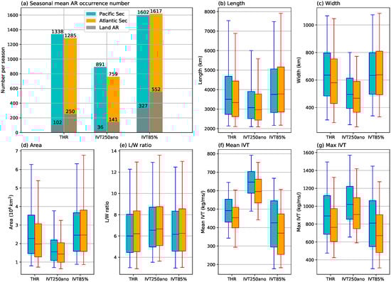
Figure 1.
(a) Average seasonal AR occurrences during the November–April season of November 2004 to April 2010 period reported by the three detection methods. The number for the North Pacific (Atlantic) sector is shown in cyan (orange). In each sector, the number of ARs that have their centroids located over land area are shown as grey shading. (b–g) are the distributions of length (km), width (km), area ( km), length/width ratio (km/km), average IVTwithin AR (kg/m/s), and the maximum IVT (kg/m/s) within AR.
Methods show considerable discrepancy in the average seasonal AR occurrences (Figure 1a). Note that the occurrence numbers are taking into account all 6-hourly time steps during the study period, therefore are dependent on the temporal resolution of data. The THR method reports an average of 1338 Pacific sector (1285 Atlantic) AR occurrences during the November–April season, () more than the IVT250ano method. IVT85% reports 1602 Pacific and 1617 Atlantic occurrences, about the double of those by IVT250ano. This method also reports notably greater number of land ARs in both sectors. This is essentially due to the design choice of taking the 85th percentile as a relative magnitude threshold. Implications of this feature will be discussed further later. Also note that after subtracting the land ARs, the THR and IVT85% methods have nearly identical AR occurrences in both basins.
Notable differences between methods are also observed in the AR geometries and IVT intensities. In general, the IVT85% ARs have the greatest length (Figure 1b), width (Figure 1c) and area (Figure 1d), followed closely by the THR ARs. The differences in length/width (L/W) ratio are smaller, with all three methods report a median L/W ratio at or slightly above 6 (Figure 1e). Orderings in the mean and maximum IVT are the opposite to that of AR sizes: IVT250ano has the highest mean (Figure 1f) and maximum (Figure 1g) AR IVT values, followed by THR. Larger sized ARs appear to have lower mean IVT values. Although the maximum IVT follows the similar trend the differences are smaller. This is because the spatial averaging process over the regions of larger sized ARs creates lower mean values, while leaving the maximum value intact. Consequently, the lower mean IVT values of THR ARs are partially due to their larger sizes, in addition to the inclusion of some weaker systems. On the other hand, it is consistent for all three methods that Pacific ARs have notably stronger mean as well as maximum IVTs than the Atlantic counterparts.
Two selected AR cases are given in Figure 2 to better explain the observed number and shape differences. Figure 2a shows that the AR over the Northeastern Pacific is detected by both the THR method (shown by green contour) and the IVT250ano method (shown by solid black contour). However, the one over the Northwestern Pacific is detected by the THR but missed by IVT250ano. This is because the area above the anomalous 250 kg/m/s IVT threshold (shown by hatching) is too small. This particular AR is not detected by IVT250ano until 12 h later, as shown in Figure 2b. However, at the same time, the one over the Northeastern Pacific is missed. These highlight one limitation of the prescribed magnitude threshold method that weaker systems, some of which correspond to the genesis or dissipating stages of well established ARs, tend to be omitted. This is because a globally applied, prescribed threshold can not adjust to the varying AR strengths very well. When coupled with a certain geometrical extent requirement (minimal area and/or length), the interaction between the magnitude-based selection and geometrical filtering tend to screen out some weaker systems. This sensitivity has been highlighted in [,].
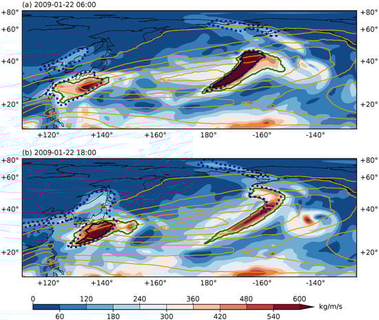
Figure 2.
IVT distributions (in kg/m/s) at the time of (a) 22 January 2009 06 UTC and (b) 22 January 2009 18 UTC over the North Pacific. ARs identified by the THR method are drawn in green contours, those by the IVT250ano method solid black contours, and those by the IVT85% method dashed black contours. Hatching indicates the regions where the IVT anomalies are above the 250 kg/m/s threshold. Orange contours are the contours of the 85th IVT percentile of the month January 2009. Contours have an interval of 100 kg/m/s. Only the pattern is shown, and the labelling of these contours are omitted for brevity.
In contrary, the THR method displays greater adaptability to varying IVT strengths. This is achieved by switching the filtering process from direct magnitude thresholding, to a filtering on the spatio-temporal “spikiness” of transient IVT plumes. Weaker but still sizable systems, as long as they stand out from the typical synoptic spatio-temporal scales, get a higher chances of being identified. Also note that the THR ARs tend to have larger sizes than the IVT250ano ones, this is because the lateral extend of the latter ARs is constrained by the selected IVT threshold, and the region immediately outside the 250 kg/m/s anomaly level is by design omitted. Such areas can be more reliably retained by the THR method. As shown in Figure 2, when both THR and IVT250ano detect a same AR, the THR boundary is wider, covering more of the strong IVT signals. This has important implications when quantifying the seasonally accumulated IVT contributions, as discussed later.
On the other hand, the IVT85% method also displays enhanced sensitivity to weaker systems, by applying a relative magnitude threshold instead of a prescribed one. For instance, the Northwestern Pacific AR is detected, as shown by the dashed black contour. However, it still misses a large portion of the Northeast Pacific AR in Figure 2b. This is because the 85th percentile itself is not a uniform distribution, with notably higher absolute values inside storm tracks (as shown by the orange contours in Figure 2). This implies some inherent contradictions between the definition of percentiles and ARs. Firstly, the percentile values are computed on a grid-per-grid bases, with no requirement for inter-grid associations. However, ARs are defined as spatially organized regions at instantaneous time points. Furthermore, the percentiles are computed using observations spanning a very long period (a 9-year moving window with 3-months in each year in this study), and the computed percentiles are kept constant for each month. This implies that for ARs that are at constant changes, the percentiles are practically a static distribution with no day-to-day variations except when going from the end of a month to the beginning of the next. Then the strong gradients around the edges of storm tracks in the 85th percentile distribution makes it easier for moisture plumes on the edge of the storm tracks to be included into an existing AR, while setting a higher standard inside the storm tracks. This may explain the exclusive IVT85% ARs over Northeast Asia and Alaska at both of the selected time points, and the missed portion in the Northeastern Pacific AR in Figure 2b.
3.2. Life Cycle of Northern Hemisphere AR Tracks
Having identified ARs at individual time points, the algorithm introduced in Section 2.4 is applied to all Northern Hemisphere ARs detected by the three methods to form AR tracks. Only tracks lasting longer than 24 h are retained. Depending on the AR centroid at genesis time, those lying within E–100 W are labeled Pacific, and those within W–20 E Atlantic. Minimum length requirement is relaxed to 800 km, but it is required that the AR reaches ≥2000 km for at least one time step during its lifetime. Also note that the track duration is defined as the lifetime of individual ARs and is distinct from a per-grid, Eularian definition as in, for instance, [,,,], which measures the contiguous time spans when a grid cell experiences AR occurrences.
The average seasonal track numbers and durations are summarized in Figure 3. Among the three methods, THR retains the greatest number of AR tracks, with 77 (89) North Pacific (Atlantic) tracks per season, 20 (30) more than IVT250ano (Figure 3a). Despite of the greatest number of occurrences, the IVT85% method reports 74 Pacific and 71 Atlantic tracks. This is largely because many of the IVT85% ARs are less persistent systems and get filtered out by the minimal 24 h duration requirement. On the other hand, tracks found by THR last longer than the other two in both basins (Figure 3b), suggesting the greater tolerance to varying AR strengths of the THR method so that genesis and dissipation stages can be better retained, consistent with previous discussions.
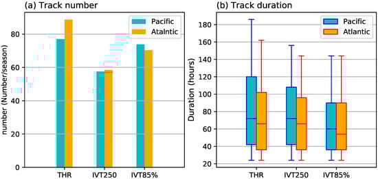
Figure 3.
(a) average number of AR tracks per cool season in the North Pacific (cyan) and North Atlantic (orange) as found by THR, IVT250ano and IVT85% methods. (b) Box-whisker plots of track durations (in hours) for the North Pacific (cyan) and North Atlantic (orange) ARs. Box ends denote the inter-quantile-range of the distribution, with the median as the line in the middle. Box whiskers denote the 5th and 95th percentiles.
As mentioned previously, ARs are associated with the warm conveyor belt of extratropical cyclones [,,,], therefore consistency should be expected between AR tracks and storm tracks in their numbers and durations. In the work of [], an ensemble of 15 extratropical cyclone tracking methods are collected to estimate the cyclone track numbers in each Hemisphere. The average DJF track number in the Northern Hemisphere is found to range from 57 to 205, with a mean of 124. Assuming relatively equal distribution in the winter season, this corresponds to about 95–341 cyclone tracks during Nov-April. Therefore, for all three methods, the combined Pacific and Atlantic track numbers are broadly consistent with the extratropical cyclone track numbers.
The medians of Pacific track durations from the THR and IVT250ano methods are about 73 h, slightly longer than the Atlantic counterparts. Pacific and Atlantic durations are about the same as the mean cyclone track durations estimated in [], who compiled cyclone tracking results from 13 different methods during a 31-year period. The median durations of Pacific (Atlantic) AR tracks reported by the IVT85% method is about 60 (55) h, which is about same as the lowest average cyclone track duration in the [] compilation. It should be noted that although closely related, there does not exist a strict one-to-one correspondence between ARs and cyclones, and the latter are also commonly found over continental regions. However, the agreement between cyclone and AR track numbers and durations lends further supports to their physical relationships.
Then the genesis and dissipation locations of AR tracks found by the three methods, quantified as number of occurrences per season are shown in Figure 4. The THR (Figure 4a) and IVT250ano (Figure 4c) methods both indicate two AR genesis hot spots over the western boundary warm current regions—the Kuroshio current for Pacific and Gulf Stream for Atlantic. Both also have considerable extensions into the basin interior. These are regions of active air-sea interactions with semi-permanent upward latent and sensible heat fluxes [,], and they also correspond to the preferred cyclogenesis locations in both basins [,]. For Atlantic, a considerable number of ARs also originate from the Gulf of Mexico and pass over the southeastern America.
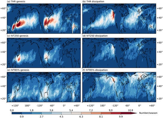
Figure 4.
Distribution of genesis (a,c,e) and dissipation (b,d,f) occurrences of AR tracks found by THR method (a,b), IVT250ano (c,d) and IVT85% (e,f) method. Only tracks longer than 24 h are included. The binary mask of the first/last AR record during the lifetime is recorded as its genesis/dissipation location, and the total accumulation number is divided into the six November–April seasons during the period 2004–2010.
The dissipation maps of THR (Figure 4b) and IVT250ano (Figure 4d) display concentrated occurrences on the opposite side of the basins. Dissipation locations over Atlantic are more spread-out and reach higher latitudes than over Pacific, largely due to the lack of long mountain barriers along the western coast of North America that terminate most Pacific ARs abruptly. The genesis and dissipation patterns agree well with those in [], who used a 4-dimensional object-orientated algorithm to locate and track strong and sustaining IVT “footprints”. The general AR movements suggested by these patterns are also consistent with the Northern Hemisphere cyclone movements over the two ocean basins (e.g., [,,]).
IVT85% suggests more uniform genesis and dissipation distributions (Figure 4e). Both genesis and dissipation locations have a wider meridional spread and penetrate deeper into the continents. This is consistent with the design choice of taking the 85th percentile value as the threshold, as discussed previously. The pattern of genesis locations is also similar to that of the “short AR events” category (tracks short than 24 h) of [], who used an areal overlap ratio based tracking method. Therefore, it may be inferred that the IVT85% method here tends to retain shorter-lived AR tracks that terminate not too far away from their genesis locations, this is also consistent with its overall lower track durations shown in Figure 3. On the other hand, the deeper continent penetration of this method may render it a better choice for landfalling related studies, where the potential inland impacts from ARs can be captured to the fullest.
Lastly, note that the THR method reports an additional genesis hot spot in the middle east around the Red Sea (this can also be seen in the IVT85% result), and another even weaker one over west Siberia. These should not be termed ARs as they are likely governed by distinct physical mechanisms. However, these are well organized (above thousand kilometers in length) and relatively persistent (can be tracked over 24 h) water plumes. The identification of such systems speaks to the greater adaptability of the THR method, and its ability in encompassing a wider range of transient water vapor plumes in a single framework.
To give a closer look at the strength and length evolutions of AR tracks, tracks with durations between 30–120 h are selected and temporally interpolated to a life cycle of 0–100%. This subset accounts for 66–76% (75–80%) of all Pacific (Atlantic) tracks among different methods. Statistics based on tracks with durations of 48–84 h, where better compatibility in the temporal interpolation is achieved, reveal qualitatively consistent results.
Figure 5a,d,g show the evolutions of mean IVT in ARs found by the three methods. IVT250ano has the highest mean IVT, followed by THR, consistent with Figure 1. THR and IVT250ano methods indicate a ∼46–64 kg/m/s strengthening in mean IVT, and a subsequent weakening during the 2nd half of the life cycle for both basins. The strengthening is significant with p-values ≤ 0.01 by a 2-tailed Wilcoxon-Mann-Whitney (WMW) test []. The preference of WMM over a Student’s t test is because the positive-definite IVT and length distributions have a longer right tail and are not Gaussian. IVT85% tracks intensify by ∼38–60 kg/m/s but weaken more significantly at the end of life cycle compared with the beginning. The timing of peak mean IVT also shows some differences. THR tracks reach peak mean IVT slightly after mid-time, while IVT250ano (IVT85%) tracks reach peak at about 40 % (30%) for both basins. The evolution of maximum IVT (Figure 5b,e,h) are qualitatively the same but with amplified magnitude ranges. Note that both mean and maximum IVT evolutions suggest a stronger Pacific AR track, particularly for the maximum achievable IVT where a Pacific track is in general ∼117–140 kg/m/s stronger than an Atlantic one at their peak times. The differences are significant with p-values ≤ 0.01 in a 2-tailed Wilcoxon-Mann-Whitney test, indicated by the black triangles in the plots.
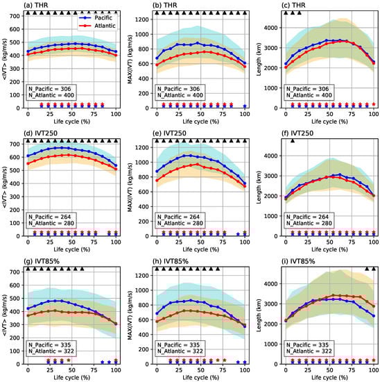
Figure 5.
Lifetime evolution of mean AR IVT (left column, in kg/m/s), maximum AR IVT (middle column, in kg/m/s) and AR axis length (right column, in km) computed from AR tracks by the THR (top row), IVT250ano (middle row) and IVT85% method (bottom row). Tracks with durations of 30–120 h are selected and normalized to 0–100% life cycle. Blue (red) curve denotes the median among Pacific (Atlantic) tracks, and cyan (yellow) shading denotes the inter-quantile range. The number of tracks are labeled at bottom left. Blue (red) stars at the bottom indicate that the distribution among Pacific (Atlantic) tracks at this time point is significantly different (with p-values ≤ 0.01) from the 1st time point at 0% life cycle. Black triangles at top indicate significant (p-values ≤ 0.01) difference between Pacific and Atlantic tracks. Significant tests are done using a 2-tailed Wilcoxon–Mann–Whitney test.
This basin difference largely disappears in the length evolution and ARs have comparable lengths in both basins during most of the life cycle. (Figure 5c,f,i). This is also consistent with results shown in Figure 1. Among the three methods, ARs tend to grow in length by 1100–1290 km then decay back to around the original level. Also note that there appears to be a phase shift in the timing of peak intensity versus peak length. ARs tend to reach the maximum IVT prior to the mid-time then start to weaken slowly, at the same time keep on growing in length till ∼60% of the life cycle, then experience a faster shortening process. An exception to this is the IVT85% Pacific tracks that the length growth starts sooner and reaches peak length at mid-time, however, it still lags behind the peak intensity. Note that the beginning stage of an extratropical cyclone is also frequently characterized by a rapid intensification, manifested as a faster deepening rate of the minimum sea level pressure (SLP) of the cyclone []. Considering the close physical correspondences between these two types of systems, the earlier peak IVT timing identified here may be related to the SLP deepening timing of cyclones. More evidences are needed to further validate this speculation.
3.3. Seasonal Accumulations of AR-Related IVT
Differences in AR occurrences could lead to differences in their accounted horizontal moisture transports. The average seasonal IVT accumulations attributed to ARs are shown in Figure 6. The numbers are computed as per-grid integrals of the IVTs within AR regions, then evenly divided into seasons.
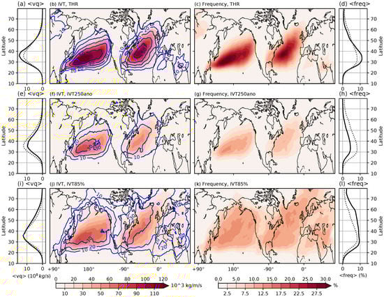
Figure 6.
(b,f,j) show the IVT accumulations (in kg/m/s) attributed to ARs detected by the THR (top row), the IVT250ano (mid row) and IVT85% (bottom row) methods. Solid blue contours show the percentage of AR-related IVT to the seasonal total. Contours are labelled with an interval of . (c,g,k) are the average seasonal AR occurrence frequencies (%) of the three methods. Occurrence frequency is defined as the fraction of all time steps during the November–April season when a grid cell is included in an AR region. Left most column (a,e,i) shows as profiles the mean seasonal zonal averages of meridional fluxes (in kg/s) by ARs detected by the three methods. And right column (d,h,l) shows the zonal average frequencies corresponding to the occurrence frequency distributions. Grey dotted curves in side profiles are the averages of the three methods. All data are averaged during the November–April seasons of November 2004 to April 2010.
The THR method shows the highest seasonal IVT accumulations over two southwest-northeast oriented bands over the oceans, centered around ∼35–40 N, where accumulation values amount to about 100–120 kg/m/s (Figure 6b). The pattern correlates well with the AR occurrence frequencies (Figure 6c), which is defined as the fraction of all time steps during the November–April season when a grid cell is included in an AR region. The distribution of the AR tracks is similar to the wintertime storm tracks in that both have a southwest-northeast orientation, with the Atlantic sector having a steeper tilt into the high latitudes []. According to the THR results, the North Pacific and North Atlantic AR track regions experience an AR about 17–25% of the time during Nov-April on average, with highest frequencies go up to ∼30%. This is in good agreement with the peak extratropical cyclone frequency climatology estimated by [], who defined cyclone frequency as the fraction of time steps when a grid cell is included in the outermost closed SLP contour enclosing a local SLP minimum. Compared with frequency statistics defined using cyclone centers, this is a more compatible definition as the AR frequency definition used in this study. However, it should be noted that the storm tracks and AR tracks do not overlap completely, with the latter being located more equatorward by about 10 degrees of latitude []. The solid blue contours in Figure 6b show the percentage of AR-related IVT with respect to the seasonal total. ARs detected by the THR method account for 20–50% of all IVT fluxes within the AR track regions.
Results from the IVT250ano method show similar patterns but with reduced magnitudes (Figure 6f). Accumulations of IVT in AR tracks are about half of the THR estimates. This is a combined result of lower AR occurrence frequencies, as shown in Figure 6g, and the detected ARs having smaller sizes, as shown previously in Section 3.1. The relative importance of these two factors will be discussed further later.
The IVT85% method also shows higher IVT accumulations over the AR tracks, but with considerable wider spreads along the edges and into the continents (Figure 6j). This could be explained by the rather uniform occurrence frequency distribution in Figure 6k, which in turn may be attributed to the design choice of taking the 85th percentile as a relative threshold. However, IVT values within the AR tracks are notably stronger, therefore an AR (or the part of the AR) in the interior of the AR track contributes more to the IVT accumulations than one (or the part) on the perimeter of the AR track. Consequently, the occurrence frequencies are more uniform than the IVT accumulations.
ARs have been found to be the primary contributor to the mid-latitude poleward moisture transport [,]. The profiles in the left column of Figure 6 display the zonal averages of the meridional fluxes () attributed to ARs in different methods. Note that the meridional moisture flux is multiplied by the grid cell zonal length to give a unit of kg/s. In the computation of the meridional flux, neither the meridional wind nor specific humidity undergoes any temporal filtering. This is because it has been demonstrated that the conventional transient perturbation formulation defined as the covariance of transient wind and humidity terms does not give a proper attribution to AR-related meridional fluxes [].
It can be seen that ARs contribute to the meridional moisture fluxes mostly within the latitudinal band of 25–45 N, with a peak at around N, consistent with results from [,]. At this latitude, THR ARs account for the highest meridional flux, at about kg/s, followed by IVT85%. North of N, the importance of THR- and IVT250ano- ARs starts to decline, while the fluxes by IVT85% ARs show a slower decrease with latitude. This is consistent with the more uniform occurrence distribution of IVT85% ARs, as indicated by the frequency profiles in the right column of Figure 6.
To further diagnose these IVT accumulation differences, ARs detected by the THR and IVT250ano methods are paired up using their areal overlaps. Depending on whether the regions of two ARs detected by the two methods (A and B) intersect each other at a given time point, three different matching scenarios are defined:
- Only A: no areal intersection and an AR is only detected by method A.
- Only B: no areal intersection and an AR is only detected by method B.
- Paired: The region of A intersects with that of B. In such cases, the AR is regarded as detected by both methods, and the detection by method A is referred to as Paired A, and detection by method B is referred to as Paired B.
The seasonal average occurrence numbers of the three matching scenarios are given in Table 1. Only the North Pacific sector is included and the same principles also apply to the North Atlantic.

Table 1.
(a) Matching ARs found by the THR method (labeled as “A” as a shorthand) and the IVT250ano method (labeled “B”). The occurrence numbers per season for the three matching scenarios of (i) : ARs only detected by method A; (ii) : ARs only detected by method B. (iii) : ARs detected by both methods; (b) similar as in (a) but between the THR and the IVT85% methods.
Between the THR and IVT250ano methods, about 505 ARs are only found by THR and 40 are exclusive to IVT250ano ( and columns in Table 1a). Note that the difference of 505 − 40 = 465 does not equal the difference of 1338 − 891 = 447 indicated in Figure 1a, as cases where more than two ARs intersecting each other are omitted in the pairing process to avoid duplicates in statistics. The exclusive THR ARs are more concentrated over the Northwestern Pacific, where most North Pacific ARs originate. ARs at the genesis stage also tend to be weaker in intensity. The inclusion of these ARs further demonstrates the greater adaptability of the THR method to AR magnitude variations compared with a method that directly thresholds the magnitude.
However, these exclusive AR detections do not contribute significantly to the IVT accumulation differences (note the smaller-ranged color bars in Figure 7a,b), compared with the Paired A and Paired B categories (Figure 7c,d), where there are equal number of ARs in the two methods but with different spatial coverages. Therefore, the major difference in AR related IVT accumulations lies in the greater IVT values on a per-AR basis, than the greater number of exclusive THR detections. This distinction is inherently related to the structure of ARs. A typical AR resides within the warm conveyor belt of the pre-cold-frontal region of an extratropical cycle, where the sharp horizontal temperature gradient gives rise to a low level jet by the thermal wind relationship []. Strong poleward moisture fluxes carried by this low level jet are therefore confined to a narrow band of a few hundred kilometers. This explains that ARs contribute the majority of total poleward moisture transport with less than of the zonal extent of the Earth [], and also highlights the sensitivity of the AR associated moisture fluxes to the AR boundary definition. This sensitivity is also dependent on the data horizontal resolution. For instance, for the ERA-I dataset with a resolution, excluding one grid cell on each side of the AR axis corresponds to a width decrease of ∼150 km. In this regard, ARs detected by the prescribed magnitude thresholding method will tend to miss some strong signals outside of the contour defined by the threshold value. The degree of this underestimation is affected by the choice of the threshold value, which in itself has some degrees of subjectively. An arbitray threshold choice will become problematic when applied on future climate projections when the underlying IVT distribution experiences slow varying changes, or when different levels of model biases are present.
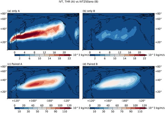
Figure 7.
Average seasonal IVT accumulations (in ) attributed to (a) ARs detected only by the method THR (labelled “A” for short, corresponds to the Only A category in Table 1a). (b) ARs detected only by the method IVT250ano (labelled “B” for short, corresponds to the Only B category in Table 1a). (c) ARs detected by method A when it is paired with an AR detected by method B (Paired A category in Table 1a). (d) ARs detected by method B when it is paired with an AR detected by method A (Paired B category in Table 1a). Note that the bottom panel uses a different colorbar.
Table 1b diagnoses the matchings between THR and IVT85% methods in a similar manner. There are a total of 989 AR occurrences that are detected by both methods. However, the 989 ARs detected by the THR method account for a greater IVT accumulation than their IVT85% counterparts (Figure 8c,d). This is partially due to the fact that the THR method achieves a more effective segmentation of strong IVT signals from the background, as supported by the stronger mean and maximum IVT values in THR ARs, even though the two sets have comparable sizes (Figure 1). Additionally, these 989 ARs detected by IVT85% have a more uniform occurrence distribution than those by the THR method (not shown), with wider spreads around the edges of the AR track region. However, outside of the AR tracks there is not much of IVT, rendering less effective contributions to the IVT accumulations. The exclusive ARs also contribute differently to these two methods. There are 268 exclusive THR ARs, mostly located within the AR track (Figure 8a), and 492 exclusive IVT85% ARs, mostly located on the perimeter of the North Pacific basin (Figure 8b), and penetrate deeper into the continents. This later feature makes IVT85% a good candidate for landfalling related studies. However, the results over open oceans suggest a weaker correspondence between AR tracks and storm tracks.
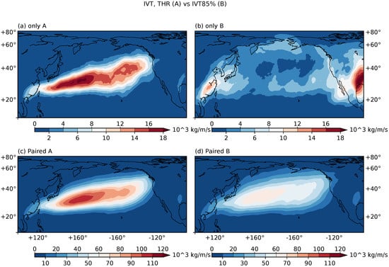
Figure 8.
Similar as Figure 7 but for matchings between the THR and IVT85% methods.
The results shed some light on the implications of AR definition on the identified role they play in the large scale poleward moisture transports: the most effective attribution to this transport does not seem to lie in the shear number of detections, but in the correct identification of the narrow band of strong IVT signals. And the magnitude thresholding methods that directly apply the filtering process on IVT values appear to underperform in this respect in comparison.
4. Summary
In this work we applied a new image-processing based AR detection and tracking method to track Northern Hemisphere ARs from the ERA-I Reanalysis dataset. Two conventional magnitude thresholding methods, one with a prescribed IVT magnitude threshold (IVT250ano) and one with a relative IVT magnitude threshold (IVT85%), are also applied on the same dataset. The results from different methods are compared, with a focus on seasonal average statistics derived from wintertime ARs in the present day climate. Uncertainties originated from methodological differences in AR related researches have been highlighted by the ARTMIP project [,,]. Individual detection methods were often devised to target some specific scientific questions, and their inherent advantages and limitations are often better revealed when putting into comparisons with each other.
The two magnitude threshold methods included in this study both have their own applications and various derivatives, for instance, a prescribed IVT threshold has been used in [,,,,], and the 85th percentile threshold has seen its applications in [,,]. The former, when applied on an anomalous field, imposes a global threshold across time; and when applied on an absolute field, loses the spatial variability as well. The lack of its flexibility introduces some potential issues when applied on data across basins, decadal time scales or beyond, and on future climate projections. The immediately observable effect is the false negative detections of some weaker systems, many of which correspond to the genesis or dissipating stages of ARs. This is usually coupled with a geometrical filtering process that more stringent geometrical criteria often lead to fewer detections []. This effect is observed in the two AR cases presented in Section 3.1. When taking the long-term average, this leads to a lower seasonal AR occurrences. On a per-AR basis, a prescribed magnitude threshold tends to omit some strong IVT signals outside of the contour determined by the threshold value. As strong IVTs associated with an AR lie mostly within a narrow band of a few hundred kilometers, any underestimate of the lateral extent of ARs can lead to a systematic underestimate of the overall moisture transport attributed to ARs.
These issues are greatly alleviated in the new THR method, by switching from a filtering on the IVT magnitude to a filtering on the spatio-temporal “spikiness” of the IVT distribution. Transient moisture plumes that stand out from the typical spatio-temporal scales of ARs get a higher chance of being identified. Consequently, the genesis and dissipating stages can be more reliably retained. On a per-AR basis, the narrow band of strong IVTs that corresponds to the low level jet of an AR is better captured. The combined effects from a greater detection number and a more effective detection of per-AR IVT render about more seasonal AR related IVT accumulations than the IVT250ano method.
Unlike the globally applied prescribed IVT threshold, the IVT85% method relies on a relative, percentile-based threshold. Although variable in space, the percentiles are by design mostly fixed in time, with a temporal step of a month as implemented in this study. Compared with the fast changing synoptic conditions that ARs are embedded, this is practically a static distribution, with strong gradients around the edges of AR tracks. Lower percentile values outside of the AR tracks therefore create a more uniform AR occurrence distribution, with more detected ARs on the perimeter of AR tracks and with deeper penetration into the continents. This makes it a good candidate for landfalling related studies. However, many of these ARs detected by this method appear to be weaker in intensities and less persistent in time. This is manifested in the smaller number of identified AR tracks and shorter track durations compared with the other two methods. The genesis and dissipation locations of thus detected AR tracks are also less coherent with the storm tracks.
On the other hand, all examined methods are capable of capturing some key elements of ARs, and good agreements are found in the length/width ratio of the detected ARs, stronger North Pacific ARs than North Atlantic ones, and more AR-related IVT accumulations within storm track regions in both ocean basins. The detected seasonal average AR tracks and track durations are also within the estimated range of extratropical cyclone numbers and durations from previous studies. Consistent for all three methods, both basins have their own preferred AR genesis locations: Kuroshio warm current region and its extension for North Pacific, and the Gulf of Mexico and the Gulf stream region for North Atlantic, consistent with previous studies [,]. This is also consistent with the preferred extratropical cyclone genesis locations []. Most ARs terminate at the opposite side of the ocean basins, and North Pacific has a more concentrated “AR graveyard” than the North Atlantic, thanks to the long mountain barriers along the western coast of North America continent.
All methods also reveal some consistent features regarding the life cycle evolutions of an AR track. The mean and maximum IVTs are found to intensify significantly, although by various degrees, to a peak value at or prior to the mid-time of their life cycle. On the other hand, the length evolution shows a delayed peak time compared with peak strength. North Pacific AR tracks are significantly stronger than North Atlantic ones but have comparable length throughout most of the AR lifetime.
This work has been mostly focused on the present day climate. Because the new THR method functions by selecting signals from the spatio-temopral scale of ARs, which is a more stable attribute than the IVT or IWV intensities. This makes the method less prone to the potential difficulties in reliably detecting ARs in a warming climate, and results from different models more readily comparable when different model biases may be present. In an ongoing project, we are examining the simulated AR responses to high resolution models as well as to future climate changes. The data cover both observations and simulations from different climate models with different configurations. The relaxation on magnitude thresholding in the detection process helps to achieve more consistent results across different experiments, and the advantage of this new method will be better demonstrated in such type of applications.
Author Contributions
Methodology, G.X. and X.M.; Software, G.X.; validation, G.X., X.M., P.C.; formal analysis, G.X., X.M., P.C., L.W.; resources, X.M., P.C.; writing—original draft preparation, G.X., X.M.; writing—review and editing, G.X., X.M., P.C., L.W.; supervision, P.C., L.W.; project administration, P.C.; funding acquisition, X.M., P.C.; All authors have read and agreed to the published version of the manuscript.
Funding
This work is supported by the National Key Research and Development Program of China with grant NO. 2017YFC1404000. This work is also supported by the National Science Foundation of China (NSFC) with grant No. 41490644 (41490640). We also received support from the NSFC grant #41776013, and National Key Research and Development Program of China grant 2017YFC1404100 and 2017YFC1404101.
Acknowledgments
This is a collaborative project between the Ocean University of China (OUC), Texas A&M University (TAMU) and the National Center for Atmospheric Research (NCAR) and completed through the International Laboratory for High Resolution Earth System Prediction (iHESP)- a collaboration by the Qingdao National Laboratory for Marine Science and Technology Development Center, Texas A&M University, and the National Center for Atmospheric Research. We are grateful to the helpful comments from Dr. Christine Shields and Dr. Chris Patricola during the course of this work, and two anomymous reviewers during the peer review stage.
Conflicts of Interest
The authors declare no conflict of interest. The funders had no role in the design of the study; in the collection, analyses, or interpretation of data; in the writing of the manuscript, or in the decision to publish the results.
References
- Zhu, Y.; Newell, R.E. A Proposed Algorithm for Moisture Fluxes from Atmospheric Rivers. Mon. Weather Rev. 1998, 126, 725–735. [Google Scholar] [CrossRef]
- Bao, J.W.; Michelson, S.A.; Neiman, P.J.; Ralph, F.M.; Wilczak, J.M. Interpretation of Enhanced Integrated Water Vapor Bands Associated with Extratropical Cyclones: Their Formation and Connection to Tropical Moisture. Mon. Weather Rev. 2006, 134, 1063–1080. [Google Scholar] [CrossRef]
- Gimeno, L.; Nieto, R.; Vázquez, M.; Lavers, D. Atmospheric rivers: A mini-review. Front. Earth Sci. 2014, 2, 2. [Google Scholar] [CrossRef]
- Dettinger, M. Climate Change, Atmospheric Rivers, and Floods in California—A Multimodel Analysis of Storm Frequency and Magnitude Changes1. JAWRA J. Am. Water Resour. Assoc. 2011, 47, 514–523. [Google Scholar] [CrossRef]
- Ralph, F.M.; Neiman, P.J.; Kiladis, G.N.; Weickmann, K.; Reynolds, D.W. A Multiscale Observational Case Study of a Pacific Atmospheric River Exhibiting Tropical–Extratropical Connections and a Mesoscale Frontal Wave. Mon. Weather Rev. 2011, 139, 1169–1189. [Google Scholar] [CrossRef]
- Ralph, F.M.; Neiman, P.J.; Wick, G.A. Satellite and CALJET Aircraft Observations of Atmospheric Rivers over the Eastern North Pacific Ocean during the Winter of 1997/98. Mon. Weather Rev. 2004, 132, 1721–1745. [Google Scholar] [CrossRef]
- Neiman, P.J.; Ralph, F.M.; Wick, G.A.; Lundquist, J.D.; Dettinger, M.D. Meteorological Characteristics and Overland Precipitation Impacts of Atmospheric Rivers Affecting the West Coast of North America Based on Eight Years of SSM/I Satellite Observations. J. Hydrometeorol. 2008, 9, 22–47. [Google Scholar] [CrossRef]
- Hagos, S.; Leung, L.R.; Yang, Q.; Zhao, C.; Lu, J. Resolution and Dynamical Core Dependence of Atmospheric River Frequency in Global Model Simulations. J. Clim. 2015, 28, 2764–2776. [Google Scholar] [CrossRef]
- Rutz, J.J.; Steenburgh, W.J.; Ralph, F.M. Climatological Characteristics of Atmospheric Rivers and Their Inland Penetration over the Western United States. Mon. Weather Rev. 2014, 142, 905–921. [Google Scholar] [CrossRef]
- Rutz, J.J.; Steenburgh, W.J.; Ralph, F.M. The Inland Penetration of Atmospheric Rivers over Western North America: A Lagrangian Analysis. Mon. Weather Rev. 2015, 143, 1924–1944. [Google Scholar] [CrossRef]
- Lavers, D.A.; Villarini, G.; Allan, R.P.; Wood, E.F.; Wade, A.J. The detection of atmospheric rivers in atmospheric reanalyses and their links to British winter floods and the large-scale climatic circulation. J. Geophys. Res. Atmos. 2012, 117. [Google Scholar] [CrossRef]
- Nayak, M.A.; Villarini, G.; Lavers, D.A. On the skill of numerical weather prediction models to forecast atmospheric rivers over the central United States. Geophys. Res. Lett. 2014, 41, 4354–4362. [Google Scholar] [CrossRef]
- Guan, B.; Waliser, D.E. Detection of atmospheric rivers: Evaluation and application of an algorithm for global studies. J. Geophys. Res. Atmos. 2015, 120, 12514–12535. [Google Scholar] [CrossRef]
- Vincent, L. Morphological grayscale reconstruction in image analysis: Applications and efficient algorithms. IEEE Trans. Image Process. 1993, 2, 176–201. [Google Scholar] [CrossRef] [PubMed]
- Ralph, F.M.; Wilson, A.M.; Shulgina, T.; Kawzenuk, B.; Sellars, S.; Rutz, J.J.; Lamjiri, M.A.; Barnes, E.A.; Gershunov, A.; Guan, B.; et al. ARTMIP-early start comparison of atmospheric river detection tools: How many atmospheric rivers hit northern California’s Russian River watershed? Clim. Dyn. 2018, 52, 4973–4994. [Google Scholar] [CrossRef]
- Mundhenk, B.D.; Barnes, E.A.; Maloney, E.D. All-Season Climatology and Variability of Atmospheric River Frequencies over the North Pacific. J. Clim. 2016, 29, 4885–4903. [Google Scholar] [CrossRef]
- Neu, U.; Akperov, M.G.; Bellenbaum, N.; Benestad, R.; Blender, R.; Caballero, R.; Cocozza, A.; Dacre, H.F.; Feng, Y.; Fraedrich, K.; et al. Imilast: A community effort to intercompare extratropical cyclone detection and tracking algorithms. Bull. Am. Meteorol. Soc. 2013, 94, 529–547. [Google Scholar] [CrossRef]
- Dee, D.P.; Uppala, S.M.; Simmons, A.J.; Berrisford, P.; Poli, P.; Kobayashi, S.; Andrae, U.; Balmaseda, M.A.; Balsamo, G.; Bauer, P.; et al. The ERA-Interim reanalysis: Configuration and performance of the data assimilation system. Q. J. R. Meteorol. Soc. 2011, 137, 553–597. [Google Scholar] [CrossRef]
- Shields, C.A.; Rutz, J.J.; Leung, L.Y.; Ralph, F.M.; Wehner, M.; Kawzenuk, B.; Lora, J.M.; McClenny, E.; Osborne, T.; Payne, A.E.; et al. Atmospheric River Tracking Method Intercomparison Project (ARTMIP): Project goals and experimental design. Geosci. Model Dev. 2018, 11, 2455–2474. [Google Scholar] [CrossRef]
- Mahoney, K.; Jackson, D.L.; Neiman, P.; Hughes, M.; Darby, L.; Wick, G.; White, A.; Sukovich, E.; Cifelli, R. Understanding the Role of Atmospheric Rivers in Heavy Precipitation in the Southeast United States. Mon. Wea. Rev. 2016, 144, 1617–1632. [Google Scholar] [CrossRef]
- Dettinger, M.D. Atmospheric Rivers as Drought Busters on the U.S. West Coast. J. Hydrometeorol. 2013, 14, 1721–1732. [Google Scholar] [CrossRef]
- Sellars, S.L.; Kawzenuk, B.; Nguyen, P.; Ralph, F.M.; Sorooshian, S. Genesis, Pathways, and Terminations of Intense Global Water Vapor Transport in Association with Large-Scale Climate Patterns. Geophys. Res. Lett. 2017, 44, 12465–12475. [Google Scholar] [CrossRef]
- Wernli, H. A lagrangian-based analysis of extratropical cyclones. II: A detailed case-study. Q. J. R. Meteorol. Soc. 1997, 123, 1677–1706. [Google Scholar] [CrossRef]
- Rudeva, I.; Gulev, S.K.; Simmonds, I.; Tilinina, N. The sensitivity of characteristics of cyclone activity to identification procedures in tracking algorithms. Tellus A Dyn. Meteorol. Oceanogr. 2014, 66, 24961. [Google Scholar] [CrossRef]
- Yu, L.; Jin, X.; Weller, R.A. Multidecade Global Flux Datasets from the Objectively Analyzed Air-sea Fluxes (OAFlux) Project: Latent and Sensible Heat Fluxes, Ocean Evaporation, and Related Surface Meteorological Variables; OAFlux Project Technical Report; OA-2008-01; Woods Hole Oceanographic Institution: Falmout, MA, USA, 2008; pp. 1–64. [Google Scholar]
- Kelly, K.A.; Small, R.J.; Samelson, R.M.; Qiu, B.; Joyce, T.M.; Kwon, Y.O.; Cronin, M.F. Western boundary currents and frontal air-sea interaction: Gulf stream and Kuroshio Extension. J. Clim. 2010, 23, 5644–5667. [Google Scholar] [CrossRef]
- Wernli, H.; Schwierz, C. Surface Cyclones in the ERA-40 Dataset (1958–2001). Part I: Novel Identification Method and Global Climatology. J. Atmos. Sci. 2006, 63, 2486–2507. [Google Scholar] [CrossRef]
- Hodges, K.I. A General-Method For Tracking Analysis And Its Application To Meteorological Data. Mon. Weather Rev. 1994, 122, 2573–2586. [Google Scholar] [CrossRef]
- Hodges, K.I. Feature Tracking on the Unit Sphere. Mon. Weather Rev. 1995, 123, 3458–3465. [Google Scholar] [CrossRef]
- Zhou, Y.; Kim, H.; Guan, B. Life Cycle of Atmospheric Rivers: Identification and Climatological Characteristics. J. Geophys. Res. Atmos. 2018, 123, 12715–12725. [Google Scholar] [CrossRef]
- Wilks, D.S. Statistical Methods in the Atmospheric Sciences; Academic Press: Cambridge, MA, USA, 2011; Volume 100. [Google Scholar]
- Rutz, J.J.; Shields, C.A.; Lora, J.M.; Payne, A.E.; Guan, B.; Ullrich, P.; O’Brien, T.; Leung, L.R.; Ralph, F.M.; Wehner, M.; et al. The Atmospheric River Tracking Method Intercomparison Project (ARTMIP): Quantifying Uncertainties in Atmospheric River Climatology. J. Geophys. Res. Atmos. 2019, 124, 13777–13802. [Google Scholar] [CrossRef]
- Guan, B.; Waliser, D.E. Tracking Atmospheric Rivers Globally: Spatial Distributions and Temporal Evolution of Life Cycle Characteristics. J. Geophys. Res. Atmos. 2019, 124, 12523–12552. [Google Scholar] [CrossRef]
- Zhou, Y.; Kim, H. Impact of Distinct Origin Locations on the Life Cycles of Landfalling Atmospheric Rivers Over the U.S. West Coast. J. Geophys. Res. Atmos. 2019, 124, 11897–11909. [Google Scholar] [CrossRef]
© 2020 by the authors. Licensee MDPI, Basel, Switzerland. This article is an open access article distributed under the terms and conditions of the Creative Commons Attribution (CC BY) license (http://creativecommons.org/licenses/by/4.0/).