Abstract
Stratocumulus clouds have a distinctive structure composed of a combination of lumpy cellular structures and thin elongated regions, resembling canyons or slits. The elongated slits are referred to as “spiderweb” structure to emphasize their interconnected nature. Using very high resolution large-eddy simulations (LES), it is shown that the spiderweb structure is generated by cloud-top evaporative cooling. Analysis of liquid water path (LWP) and cloud liquid water content shows that cloud-top evaporative cooling generates relatively shallow slits near the cloud top. Most of liquid water mass is concentrated near the cloud top, thus cloud-top slits of clear air have a large impact on the entire-column LWP. When evaporative cooling is suppressed in the LES, LWP exhibits cellular lumpy structure without the elongated low-LWP regions. Even though the spiderweb signature on the LWP distribution is negligible, the cloud-top evaporative cooling process significantly affects integral boundary layer quantities, such as the vertically integrated turbulent kinetic energy, mean liquid water path, and entrainment rate. In a pair of simulations driven only by cloud-top radiative cooling, evaporative cooling nearly doubles the entrainment rate.
1. Introduction
Stratocumulus (Sc) clouds form near the surface, covering about 20% the Earth’s surface. Sc have a large effect on the Earth’s energy balance. Small variations in Sc area coverage can produce energy-balance changes comparable to those generated by greenhouse gases (e.g., [1,2,3,4]). Sc have a distinctive structure composed of a combination of lumpy cellular structures and thin elongated regions, resembling canyons or slits. See, for instance, observations in Figure 1 and additional observations in Figure 1 of [5] and Figures 5 and 6 of [6]. This characteristic Sc structure is also reproduced in some large-eddy simulations (LES) [7,8,9]. The cloud structure registers in the radiance fields in observations (Figure 1) and liquid water path (LWP) in model data. In the present study, of primary interest are the thin elongated regions. We refer to these structures as spiderweb to emphasize their interconnected nature. Spiderweb types vary greatly by spider species. Even though spiral orb webs are often depicted, webs can be irregular. The stratocumulus cloud-top slits loosely resemble the internal structure of webs made by hackledmesh weavers, i.e., members of the spider family Amaurobiidae. The term spiderweb is used in a broad sense without implying true representation of either part or all of any web produced by a spider.
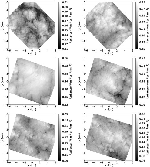
Figure 1.
Radiance fields from six observed stratocumulus scenes during the ORACLES campaign. All images are nadir views of the band aquired by the Airborne Multiangle SpectroPolarimetric Imager (AirMSPI) on 22 September 2016 off the coast of Namibia. In spite of variation in cloud cover, the characteristic stratocumulus structure composed of cellular blobs and thin spiderweb-like slits is visible.
The objective of the present study is to understand the physical processes that create the Sc spiderweb structure. Sc radiative properties depend on the liquid water spatial structure. In turn, the cloud liquid water spatial structure is a result of a turbulent flow whose dynamics are modulated by the various physical processes, such as shear, buoyancy, phase changes, cloud microphysics, etc. The present study aspires to create direct links between the atmospheric boundary layer dynamics and cloud radiative properties by linking the effects of individual physical processes to the cloud liquid structure.
In situ observations (e.g., [10,11,12]) and high resolution LES [7,9] show complex three dimensional cloud structure. In this study, the cloud liquid water path—integrating the cloud-depth dimension to form a two-dimensional field—is primarily considered to simplify the exploration of the cloud spatial structure. Consideration of the LWP is not a significant limitation because of the stratiform nature of Sc. Only cloud macrophysical effects are considered and variations of LWP are only related to covariances of total water content, pressure, and temperature. For non-precipitating and non-drizzling Sc and model resolutions of 1–, this approximation is expected to result in sufficiently representative LWP spatial structure [9]. At smaller scales (centimeters), cloud microphysical effects can affect the local cloud liquid distribution. For instance, regions of low droplet concentration (and consequently low cloud liquid mixing ratios) can be created because of droplet inertial effects [13].
We hypothesize that two main mechanisms control the spatial LWP structure: (a) boundary-layer-deep convective motions, which create the cloud lumpy cellular structure; and (b) evaporative cooling near the cloud top, which creates the spiderweb structure. The hypothesis is based on observations of convection organization confined under an inversion (e.g., [14,15]) and visualizations of stratocumulus-top turbulence in fine-scale process-level models, e.g., ([16] Figure 3) and ([17] Figure 5). Evaporative cooling and the resulting buoyancy reversal instability (BRI) create shallow groves on the cloud top.
The working hypothesis has two important implications for Sc physics: (a) self-similarity of cloud liquid spatial structure may not hold across all scales because two different processes with different length and time scales modulate the cloud liquid distribution. For instance, Davis et al. [18] and Ma et al. [19] report a scale break in observations of Sc liquid water content at 1–; (b) attribution of cloud liquid structure to different physical processes. The importance of convective motions driven by surface buoyancy, cloud top radiative cooling, and evaporative cooling in determining structure of the stratocumulus-topped boundary layer has been extensively studied and, presently, we are not introducing any new mechanisms of turbulence generation and cloud liquid modulation. However, we aim to elucidate and, to the extent possible, to decompose the effects of cloud-top radiative and evaporative cooling. In the past, rather general terms such as “entrainment,” “radiative cooling,” and “cloud holes” have been used with somewhat indefinite meanings and, in many cases, interchangeably (e.g., [8,20,21,22,23]).
For non linear systems with a very large number of degrees of freedom (e.g., some of the present simulations utilize computational grids with 20 billion grid cells), it is challenging to attribute outcomes to specific physical processes. Thus, a series of perturbation numerical experiments is carried out to observe the impact to different physical processes on the stratocumulus-topped boundary layer. The present hypothesis is assessed by performing Sc LES without accounting for latent heat exchange. Additional LES are carried out to control for other physical parameters.
The present study is enabled by recent improvements in high-resolution model fidelity and computing power, which result in realistic validated simulations of the entire boundary layer [9,24]. The observations, numerical model, and numerical experiments are described in Section 2. Simulations are based on the DYCOMS II RF01 nocturnal non-precipitating Sc case [25] because of the relatively simple Sc physics and the availability of extensive previous LES runs and validation data. Results are presented in Section 3 where the effects of cloud top radiative cooling are examined and support for the working hypothesis is discussed. Summary and conclusions are presented in Section 4.
2. Methodology
2.1. Observations
The large-eddy simulations are informed by the Sc radiance structure captured in images from the Airborne Multi-angle Spectro-Polarimetric Imager (AirMSPI) on NASA’s Airborne ER-2 Platform [26]. A sample of the AirMSPI images is shown in Figure 1. All images correspond to radiance fields of nadir views of the band observed during the ORACLES campaign on 22 September 2016 off the coast of Namibia [27]. Further details about the instrument and campaign can be found in Xue et al. [6]. The pixel resolution is and the scenes in Figure 1 are about wide. In spite of variations of cloud cover and intensity, the characteristic spiderweb structure is present in all images. The spiderweb is not present in the corresponding coarser resolution (25-m pixels) retrieved cloud properties images, suggesting that fine spatial resolution—less than about —is critical in discerning the spiderweb Sc structure.
2.2. Model
The LES model of Matheou and Chung [28] is used. The details of the model formulation, including details of the model setup for the present stratocumulus cases, are described in Refs. [9,24]. The LES model numerically integrates the anelastic approximation of the Navier–Stokes equations [29] on an f-plane using a doubly periodic domain in the horizontal directions. Fully-conservative fourth-order (centered) finite-differences [30,31] and the Quadratic Upstream Interpolation for Convective Kinematics (QUICK) scheme [32] are used for momentum and scalar advection, respectively. The buoyancy adjusted stretched vortex subgrid-scale turbulence model [33,34,35,36,37] is used to account for the effects of unresolved turbulence motions. The third-order Runge–Kutta method of Spalart et al. [38] is used for time integration. All grids are uniform .
The simulations are based on the DYCOMS II RF01 case [39], which is a non-precipitating nearly stationary nocturnal stratocumulus-topped marine boundary layer. The flow is driven by prescribed uniform surface latent and heat fluxes, the geostrophic wind, , and cloud-top radiative and evaporative cooling. The case-specific parameterization of [39] is used for the net longwave radiative flux, which results in strong cooling in a thin layer below the cloud top and small heating near the cloud base. A uniform large-scale horizontal divergence D is used to represent the effects of the large-scale subsidence on the evolution of the boundary layer. We refer to simulations that follow the DYCOMS II RF01 case as “full physics” simulations. Validation of the full-physics simulations and further details of the present model configuration are described in Refs. [9,24].
In all simulations, the mass of cloud liquid water condensate is diagnosed based on the local saturation water mixing ratio, using the values of pressure and temperature at the center of each grid cell. Thus, no partially saturated air is allowed in each grid cell. Moreover, microphysical effects are not taken into account, such as drizzle, droplet sedimentation, and droplet inertial effects (e.g., [13]).
A modified definition of buoyancy is used in the model to suppress latent heat exchange (including evaporative cooling). Following Matheou and Teixeira [24], in the standard LES model, buoyancy is defined proportional to deviations of virtual potential temperature from its instantaneous horizontal average ,
where g is the acceleration of gravity, the basic-state density in the anelastic approximation, and the basic-state potential temperature. The virtual potential temperature is
where is the potential temperature, r and is the water vapor and liquid water mixing ratios, and and are the gas constants of dry air and water vapor. To suppress latent heat exchange, is modified,
which is similar to its definition for air without condensate with in the place of and is the total water mixing ratio.
The artificial modification of buoyancy suppresses not only evaporative cooling at the cloud top but everywhere in the cloud. Equation (3) is applied everywhere in the cloud to avoid introducing additional parameters and uncertainty. This is a limitation of the current methodology and its effects are analyzed in the next section.
Table 1 summarizes the simulations. Model runs A–E are the same as in Matheou and Teixeira [24] and follow the same naming convection. Runs L3 and M1 are counterparts of runs E3 and A1, respectively, without evaporative cooling. Based on observations, the grid resolution is for 6 runs and for runs A1 and M1. Simulations A3, B3, C3, E3, and L3 are initialized with uniform fields and ran for four hours. Simulations A1 and M1 are initialized from run A1 of [24] at and ran for 10 min (), which is about half the convective time scale, see Section 3.1. Case A1 is merely a continuation of a full-physics simulation for additional 10 min. Case M1 is a short boundary layer evolution without latent heat exchange.

Table 1.
Summary of the cases simulated. The grid spacing is denoted by . For all runs, the grid is homogeneous . The number of horizontal and vertical grid points are and , respectively. “Wind” corresponds to forcing with the geostrophic wind or no wind (i.e., no mean surface shear), and D is the large-scale divergence. The case-specific parameterization of [39] is used for the net longwave radiative flux, except Case B3 which has null radiative flux at all model levels. Cases C3, L3, and M1 use a modified buoyancy variable (Equation (3)). Surface sensible and latent heat fluxes are denoted by “prescribed” when non-zero.
Case B3 controls for the effects of radiation on a full-physics run. Cases E3 and L3 do not include surface buoyancy fluxes, i.e., convection is only driven by cloud-top negative buoyancy production. Case E3 includes both cloud-top radiative and evaporative cooling and Case L3 only radiative cooling.
3. Results
3.1. Liquid Water Path Spatial Structure
The working hypothesis is qualitatively evaluated by examining LWP and vertical planes of cloud liquid mixing ratio, . The goal is to contrast simulations with respect to (a) the presence of spiderweb structure in LWP fields, and (b) slits of clear air near the cloud top in vertical planes. Figure 2, Figure 3 and Figure 4 show LWP from all 5-m resolution runs. Figure 5 shows LWP for the high resolution cases, .
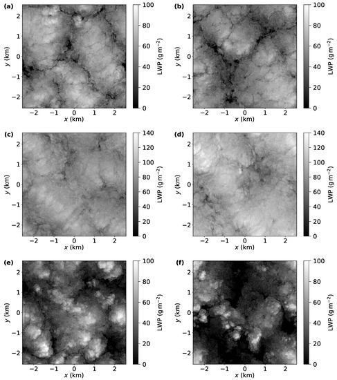
Figure 2.
Liquid water path for the run with full physics, Case A3 (a,b), run without evaporative cooling, Case C3 (c,d), and the run without radiation, Case B3 (e,f). Left column panels (a,c,e) correspond to and right column panels (b,d,f) to .
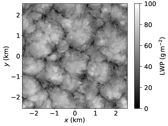
Figure 3.
Liquid water path for a run without radiation, Case B3, at .
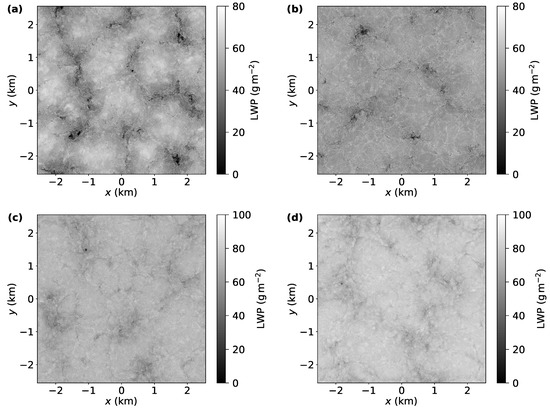
Figure 4.
Liquid water path for the runs without surface fluxes (only driven by radiation). Top panels (a,b) include the effects of evaporative cooling. Bottom panels (c,d) correspond to the run without evaporative cooling. Left column panels (a,c) correspond to and right column panels (b,d) to .
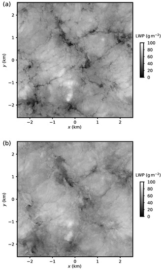
Figure 5.
Adjustment of liquid water path structure to the lack of evaporative cooling. Panel (a) shows liquid water path (LWP) from a full-physics simulation, Case A1, at , and panel (b) shows Case M1 LWP. Both simulations were initialized from a full-physics LES at and ran for 10 min. As a result of the relatively short time lapse from the common initial condition, the large-scale LWP structure is similar. The spiderweb LWP structure has shorter time scale and has dissipated in (b).
In Figure 2 and Figure 4, two time instances of LWP are shown at and . Cloud cover and LWP significantly decrease with respect to time in the case without radiation (B3), see [24]. Thus, additionally, LWP is shown in Figure 3 at . All panels in Figure 2, Figure 3 and Figure 4 exhibit the characteristic Sc lumpy structure. However, the spiderweb structure is absent from the LWP plots of cases without cloud-top evaporative cooling (Figure 2c,d and Figure 4c,d).
The contrast with respect to the spiderweb structure is higher in Cases E3 and F3, which are driven only by cloud-top radiative cooling (Figure 4), than Cases A3–C3 (Figure 2). As will be quantitatively discussed in the following sections, LWP spatial variability is still present in the cases without evaporative cooling and locations of nearly zero LWP can be observed in Figure 4c,d. However, these regions of very low LWP are not thin and elongated as in Figure 4a,b, but are broader and a few circular cloud holes are present, similar to the observations in [5].
In spite of some evidence of spiderweb structure in Figure 3, the contrast is not as strong as in Figure 4. The lack of a homogenous and high-LWP cloud, compared to other cases, may contribute to the reduced contrast.
To remove some of the effects of different boundary layer physics and evolution dynamics, LWP for Cases A1 and M1 is compared in Figure 5. Cases A1 and M1 correspond to a 10-min evolution, about half the convective time scale, of the boundary layer with and without latent heat exchange. The boundary layer convective time scale , where is the boundary layer depth and the depth-averaged vertical velocity turbulent flux. Thus, the large-scale motions remain well-correlated in Figure 5, since their time-correlation is expected to scale with . Conversely, the spiderweb dissipates in the simulation without evaporative cooling. The signature of the spiderweb is at places visible in Figure 4b, however these regions have higher LWP compared to Figure 4a.
3.2. Cloud Liquid and LWP Distributions
Figure 6 and Figure 7 show cross sections of the cloud liquid water mixing ratio for Cases A1 and M1, respectively. The cross sections correspond to vertical lines in the axes of Figure 5 passing through . The contrast between Figure 6 and Figure 7 is stronger than the corresponding LWP of Figure 5 and provides a clearer indication of the effects of evaporative cooling near the cloud top.
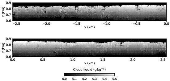
Figure 6.
Cloud liquid mixing ratio on a vertical plain at for Case A1. The elongated domain is partitioned into two panels. Only the cloudy region is shown. Evaporative cooling at the cloud top creates clear-air slits near the cloud top.
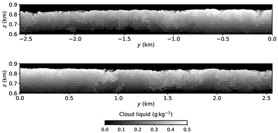
Figure 7.
Cloud liquid mixing ratio on a vertical plain at for Case M1. The elongated domain is partitioned into two panels. Only the cloudy region is shown. The cloud-top slits are absent in Case M1 (c.f., Figure 6).
As shown in previous modeling studies [16,40,41], the cloud-top slits do not extend to the entire cloud depth, but are rather concentrated near the top (see also cloud-top boundary distributions in [9]).
Examination of LWP and in Figure 5 and Figure 6 generates a key question: why do the relatively shallow cloud-top slits significantly affect the LWP structure of the entire cloud depth? Sc have most liquid content near the cloud top, thus any modification of the cloud top liquid distribution has a significant impact on the entire column.
Figure 8 shows LWP of the top-half of the cloud () and Figure 9 shows LWP of the bottom-half of the cloud for Cases A1 and M1. In other words, the sum of panels (a) of Figure 8 and Figure 9 equals the LWP contours of Figure 5a. It can be observed that a large fraction of LWP is contributed from the cloud-top region. Thus, the LWP structure, including the spiderweb, is because of variations of a relatively thin region near the cloud top.
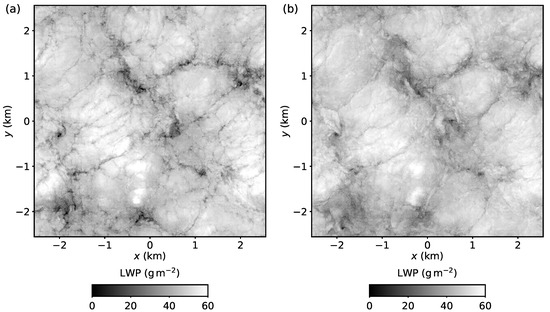
Figure 8.
Liquid water path of the top-half of the cloud: (a) Case A1, and (b) Case M1.
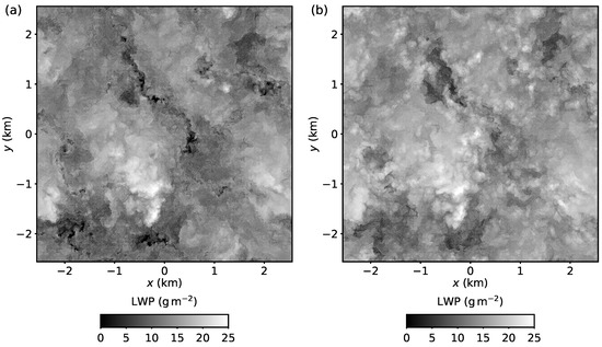
Figure 9.
Liquid water path of the bottom-half of the cloud: (a) Case A1, and (b) Case M1.
Figure 9 shows the effects of suppressing latent heat exchange in the lower part of the cloud (). Similar to Figure 5 and Figure 8, in Case M1, LWP increases in the low-LWP regions of Case A1. The lower part of the cloud has a more classical random turbulent structure without significant differences with respect to the presence of evaporative cooling (c.f., Figure 4).
Figure 10 quantifies the differences in LWP between Cases A1 and M1. For each LWP column, the pairs of LWP of Cases A1 and M1 are recorded, i.e., –. Then, joint (two-dimensional) histograms of the LWP pairs are constructed in Figure 10 for the full column LWP, cloud-top LWP (), and cloud-bottom LWP (). The histograms lay across the diagonal for perfect correlations. The histograms are not symmetric about the diagonal and spread towards the higher values of Case M1. This is consistent with the LWP contours of Figure 5, Figure 6, Figure 7, Figure 8 and Figure 9 where LWP has higher values in Case M1 compared to Case A1 at the same location. This change in LWP is observed in all values but it is larger in low-LWP regions since the contours are broader for lower x-axis values in Figure 10. The effects are also present in the lower half of the cloud. However, the amount of cloud liquid is much less in this region. Therefore, even though the effects of modified buoyancy are present in the entire cloud, any impacts in the lower half of the cloud is likely limited because of the small cloud liquid content and the more random nature of the liquid structure.
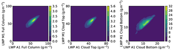
Figure 10.
Correlations between LWP distributions between Cases A1 and M1. The contours correspond to the normalized joint two-dimensional histograms of LWP. The legends correspond to probability per . The left panel corresponds to the full-column LWP, upper-half of the cloud is shown in the middle panel, and the lower-half of the cloud is shown in the right panel.
Figure 11 shows effects of suppressing latent heat exchange on the LWP Probability Density Functions (PDF) for case pairs E3–L3 and A1–M1. The LWP PDFs are compared at for Cases E3–L3 and at for Cases A1–M1. The PDFs are essentially the normalized (integrate to unity) histograms of LWP. In Cases A1 and M1 the mean LWP is approximately equal, thus the x-axis corresponds to LWP. Cases E3 and L3 have different cloud evolutions (see also next section and Figure 12), thus the x-axis is shifted by the location of the PDF mode. In both case pairs the suppression of latent heat exchange affects the left “tail” of the LWP distribution by increasing the occurrences of low LWP columns. Taking into account only the observed differences in the PDFs, we cannot conclude that the change in the PDFs is because of the spiderweb structure. However, the LWP and cloud liquid comparisons show that the spiderweb structure corresponds to low LWP cloud regions and the cases without evaporative cooling show higher liquid water content in the spiderweb region. Therefore, it is likely that the changes of the left PDF tail are mostly contributed by the spiderweb Sc structure.
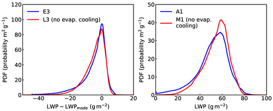
Figure 11.
Probability Density Functions (PDF) of LWP for Cases E3 and L3 (left) and A1 and M1 (right). The LWP (x-axis) in the left panel is shifted by the location of the mode of the PDF.
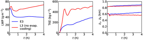
Figure 12.
Time traces of liquid water path (left panel), vertically integrated turbulent kinetic energy (middle panel), and cloud base and cloud top height for Cases E3 and L3 (right panel).
3.3. Entrainment Rate and Turbulence
Even though evaporative cooling occurs primarily at the cloud top, it affects the bulk boundary layer dynamics. Comparison of time traces in Figure 12 of simulations driven only by radiative cooling (Cases E3 and L3) shows significant changes to the vertically integrated turbulent kinetic energy (TKE), mean LWP, and entrainment rate. In Cases E3 and L3, the cloud-top evaporative cooling enhances the entrainment rate. The entrainment rate is when evaporative cooling is suppressed (Case L3) and nearly doubles to in simulations with evaporative cooling. A comparison of the Case E3 time traces with the standard DYCOMS II RF01 and other physics-perturbation experiments are documented in [24].
The reduced entrainment in Case L3 results in a cloud with more liquid water content and more radiative cooling at the cloud top. The increased radiative forcing results in more vigorous turbulence (higher TKE). Interestingly, the increase in TKE for Case L3 is not able to compensate for the lack of evaporative-cooling-generated (negative buoyancy) motions in the entrainment process. The present results suggest that entrainment is primarily affected by the nature of the cloud-top motions rather than bulk boundary layer properties.
4. Conclusions
Observations (Figure 1 and Refs. [6,12]) show that stratocumulus clouds (Sc) have a distinctive structure composed of a combination of lumpy cellular structures and thin elongated regions, resembling canyons or slits. We refer to the elongated slits as spiderweb structure. Using very high resolution ( and ) large-eddy simulations (LES) of a simple established case of a stratocumulus deck, we show that the spiderweb structure is caused by cloud-top evaporative cooling.
The effects of evaporative cooling are studied using simulations with a modified buoyancy definition, which does not account for latent heat exchange. However, cloud liquid is diagnosed in the model and used to calculate the parameterized radiative heating/cooling. The results are studied by qualitatively contrasting simulations with and without cloud-top evaporative cooling with respect to the presence of the spiderweb liquid water path (LWP) structure. Analysis of LWP of the entire cloud depth, LWP of fractions of the cloudy column, and instantaneous cloud liquid vertical planes show that cloud-top evaporative cooling generates relatively shallow slits near the cloud top. However, because most of the liquid water mass is concentrated near the cloud top, these regions of clear air have a large impact on the entire-column LWP.
The cellular Sc structure is present in simulations without latent heat exchange, suggesting that the lumpy cloud structure and circular cloud holes are generated by boundary-layer-deep convective motions. These lumpy structures are present when the boundary layer convection is driven from the top by radiative cooling, from the surface, or by a combination of the two.
In the present LES, the spiderweb structure dissipated in about ten minutes (about half the boundary layer convective time scale), suggesting that motions related to cloud-top slits generated by evaporative cooling have short time scales.
The effects of the spiderweb structure on the LWP distributions are small, and discernible only at the left tails of the distributions. This is likely because of the small area fraction of the spiderweb.
Even though the spiderweb signature on the LWP distribution is negligible, the cloud-top evaporative cooling process significantly affects integral boundary layer quantities, such as the vertically integrated turbulent kinetic energy, mean liquid water path, and the entrainment rate. In a pair of simulations driven only by cloud-top radiative cooling, evaporative cooling nearly doubles the entrainment rate.
Author Contributions
Conceptualization, G.M., A.B.D. and J.T.; methodology, G.M.; writing—original draft preparation, G.M.; writing—review and editing, A.B.D. and J.T.; modeling, G.M.; observational data, A.B.D. All authors have read and agreed to the published version of the manuscript.
Funding
This research was funded by NSF-AGS-1916619, the Office of Naval Research, Marine Meteorology Program, the NASA MAP Program, the NOAA/CPO MAPP Program, and by the DOE Office of Biological and Environmental Research, Earth and Environmental System Modeling Program.
Acknowledgments
The AirMSPI data were obtained from the NASA Langley Research Center Atmospheric Science Data Center. Computational resources supporting this work were provided by the NASA High-End Computing (HEC) Program through the NASA Advanced Supercomputing (NAS) Division at Ames Research Center. The research presented in this paper was supported by the systems, services, and capabilities provided by the University of Connecticut High Performance Computing (HPC) facility. We acknowledge informative discussions with Jerone Povner, a leading arachnologist. Part of this research was carried out at the Jet Propulsion Laboratory, California Institute of Technology, under a contract with the National Aeronautics and Space Administration.
Conflicts of Interest
The authors declare no conflict of interest.
References
- Hartmann, D.L.; Ockert-Bell, M.E.; Michelsen, M.L. The effect of cloud type on Earth’s energy balance: Global analysis. J. Clim. 1992, 5, 1281–1304. [Google Scholar] [CrossRef]
- Bretherton, C.S. Convection in stratocumulus-topped atmospheric boundary layers. In The Physics and Parameterization of Moist Atmospheric Convection; Springer: Berlin, Germany, 1997; pp. 127–142. [Google Scholar]
- Stevens, B. Atmospheric moist convection. Annu. Rev. Earth Planet. Sci. 2005, 33, 605–643. [Google Scholar] [CrossRef]
- Wood, R. Stratocumulus clouds. Mon. Weather Rev. 2012, 140, 2373–2423. [Google Scholar] [CrossRef]
- Haman, K.E. Simple approach to dynamics of entrainment interface layers and cloud holes in stratocumulus clouds. Q. J. R. Meteorol. Soc. 2009, 135, 93–100. [Google Scholar] [CrossRef]
- Xu, F.; van Harten, G.; Diner, D.J.; Davis, A.B.; Seidel, F.C.; Rheingans, B.; Tosca, M.; Alexandrov, M.D.; Cairns, B.; Ferrare, R.A.; et al. Coupled retrieval of liquid water cloud and above-cloud aerosol properties using the Airborne Multiangle SpectroPolarimetric Imager (AirMSPI). J. Geophys. Res. 2018, 123, 3175–3204. [Google Scholar] [CrossRef]
- Yamaguchi, T.; Randall, D.A. Cooling of entrained parcels in a large-eddy simulation. J. Atmos. Sci. 2012, 69, 1118–1136. [Google Scholar] [CrossRef]
- Yamaguchi, T.; Feingold, G. On the size distribution of cloud holes in stratocumulus and their relationship to cloud-top entrainment. Geophys. Res. Lett. 2013, 40, 2450–2454. [Google Scholar] [CrossRef]
- Matheou, G. Turbulence structure in a stratocumulus cloud. Atmosphere 2018, 9, 392. [Google Scholar] [CrossRef]
- Nicholls, S. The structure of radiatively driven convection in stratocumulus. Q. J. R. Meteorol. Soc. 1989, 115, 487–511. [Google Scholar] [CrossRef]
- Gerber, H.; Frick, G.; Malinowski, S.P.; Brenguier, J.L.; Burnet, F. Holes and entrainment in stratocumulus. J. Atmos. Sci. 2005, 62, 443–459. [Google Scholar] [CrossRef]
- Haman, K.E.; Malinowski, S.P.; Kurowski, M.J.; Gerber, H.; Brenguier, J.L. Small scale mixing processes at the top of a marine stratocumulus–A case study. Q. J. R. Meteorol. Soc. 2007, 133, 213–226. [Google Scholar] [CrossRef]
- Karpińska, K.; Bodenschatz, J.F.; Malinowski, S.P.; Nowak, J.L.; Risius, S.; Schmeissner, T.; Shaw, R.A.; Siebert, H.; Xi, H.; Xu, H.; et al. Turbulence-induced cloud voids: Observation and interpretation. Atmos. Chem. Phys. 2019, 19, 4991–5003. [Google Scholar] [CrossRef]
- Schmidt, H.; Schumann, U. Coherent structure of the convective boundary layer derived from large-eddy simulations. J. Fluid Mech. 1989, 200, 511–562. [Google Scholar] [CrossRef]
- Sullivan, P.G.; Patton, E.G. The effect of mesh resolution on convective boundary layer statistics and structures generated by large-eddy simulation. J. Atmos. Sci. 2011, 68, 2395–2415. [Google Scholar] [CrossRef]
- Mellado, J.P. Cloud-top entrainment in stratocumulus clouds. Annu. Rev. Fluid Mech. 2017, 49, 145–169. [Google Scholar] [CrossRef]
- Mellado, J.P.; Stevens, B.; Schmidt, H. Wind shear and buoyancy reversal at the top of stratocumulus. J. Atmos. Sci. 2014, 71, 1040–1057. [Google Scholar] [CrossRef]
- Davis, A.B.; Marshak, A.; Gerber, H.; Wiscombe, W.J. Horizontal structure of marine boundary layer clouds from centimeter to kilometer scales. J. Geophys. Res. Atmos. 1999, 104, 6123–6144. [Google Scholar] [CrossRef]
- Ma, Y.F.; Malinowski, S.P.; Karpińska, K.; Gerber, H.E.; Kumala, W. Scaling analysis of temperature and liquid water content in the marine boundary layer clouds during POST. J. Atmos. Sci. 2017, 74, 4075–4092. [Google Scholar] [CrossRef]
- Van Zanten, M.C.; Duynkerke, P.G. Radiative and evaporative cooling in the entrainment zone of stratocumulus – The role of longwave radiative cooling above cloud top. Bound.-Layer Meteorol. 2002, 102, 253–280. [Google Scholar] [CrossRef]
- Malinowski, S.P.; Andrejczuk, M.; Grabowski, W.W.; Korczyk, P.; Kowalewski, T.A.; Smolarkiewicz, P.K. Laboratory and modeling studies of cloud–clear air interfacial mixing: Anisotropy of small-scale turbulence due to evaporative cooling. New J. Phys. 2008, 10, 075020. [Google Scholar] [CrossRef][Green Version]
- Petters, J.L.; Harrington, J.Y.; Clothiaux, E.E. Radiative–dynamical feedbacks in low liquid water path stratiform clouds. J. Atmos. Sci. 2012, 69, 1498–1512. [Google Scholar] [CrossRef]
- De Lozar, A.; Mellado, J.P. Evaporative cooling amplification of the entrainment velocity in radiatively driven stratocumulus. Geophys. Res. Lett. 2015, 42, 7223–7229. [Google Scholar] [CrossRef]
- Matheou, G.; Teixeira, J. Sensitivity to physical and numerical aspects of large-eddy simulation of stratocumulus. Mon. Weather Rev. 2019, 147, 2621–2639. [Google Scholar] [CrossRef]
- Stevens, B.; Lenschow, D.H.; Vali, G.; Gerber, H.; Bandy, A.; Blomquist, B.; Brenguier, J.; Bretherton, C.; Burnet, F.; Campos, T.; et al. Dynamics and chemistry of marine stratocumulus – DYCOMS-II. Bull. Am. Meteor. Soc. 2003, 84, 579–593. [Google Scholar] [CrossRef]
- Diner, D.J.; Xu, F.; Garay, M.J.; Martonchik, J.V.; Rheingans, B.E.; Geier, S.; Davis, A.; Hancock, B.R.; Jovanovic, V.M.; Bull, M.A.; et al. The Airborne Multiangle SpectroPolarimetric Imager (AirMSPI): A new tool for aerosol and cloud remote sensing. Atmos. Meas. Tech. 2013, 6, 2007. [Google Scholar] [CrossRef]
- Zuidema, P.; Redemann, J.; Haywood, J.; Wood, R.; Piketh, S.; Hipondoka, M.; Formenti, P. Smoke and clouds above the southeast Atlantic: Upcoming field campaigns probe absorbing aerosol’s impact on climate. Bull. Am. Meteor. Soc. 2016, 97, 1131–1135. [Google Scholar] [CrossRef]
- Matheou, G.; Chung, D. Large-eddy simulation of stratified turbulence. Part II: Application of the stretched-vortex model to the atmospheric boundary layer. J. Atmos. Sci. 2014, 71, 4439–4460. [Google Scholar] [CrossRef]
- Ogura, Y.; Phillips, N.A. Scale analysis of deep and shallow convection in the atmosphere. J. Atmos. Sci. 1962, 19, 173–179. [Google Scholar] [CrossRef]
- Morinishi, Y.; Lund, T.S.; Vasilyev, O.V.; Moin, P. Fully conservative higher order finite difference schemes for incompressible flow. J. Comput. Phys. 1998, 143, 90–124. [Google Scholar] [CrossRef]
- Matheou, G.; Dimotakis, P.E. Scalar excursions in large-eddy simulations. J. Comput. Phys. 2016, 327, 97–120. [Google Scholar] [CrossRef]
- Leonard, B.P. A stable and accurate convective modelling procedure based on quadratic upstream interpolation. Comput. Methods Appl. Mech. Eng. 1979, 19, 59–98. [Google Scholar] [CrossRef]
- Lundgren, T.S. Strained spiral vortex model for turbulent fine structure. Phys. Fluids 1982, 25, 2193–2203. [Google Scholar] [CrossRef]
- Misra, A.; Pullin, D.I. A vortex-based subgrid stress model for large-eddy simulation. Phys. Fluids 1997, 9, 2443–2454. [Google Scholar] [CrossRef]
- Pullin, D.I. A vortex-based model for the subgrid flux of a passive scalar. Phys. Fluids 2000, 12, 2311–2316. [Google Scholar] [CrossRef]
- Voelkl, T.; Pullin, D.I.; Chan, D.C. A physical-space version of the stretched-vortex subgrid-stress model for large-eddy simulation. Phys. Fluids 2000, 12, 1810–1825. [Google Scholar] [CrossRef][Green Version]
- Chung, D.; Matheou, G. Large-eddy simulation of stratified turbulence. Part I: A vortex-based subgrid-scale model. J. Atmos. Sci. 2014, 71, 1863–1879. [Google Scholar] [CrossRef]
- Spalart, P.R.; Moser, R.D.; Rogers, M.M. Spectral methods for the Navier–Stokes equations with one infinite and two periodic directions. J. Comput. Phys. 1991, 96, 297–324. [Google Scholar] [CrossRef]
- Stevens, B.; Moeng, C.H.; Ackerman, A.S.; Bretherton, C.S.; Chlond, A.; De Roode, S.; Edwards, J.; Golaz, J.C.; Jiang, H.L.; Khairoutdinov, M.; et al. Evaluation of large-eddy simulations via observations of nocturnal marine stratocumulus. Mon. Weather Rev. 2005, 133, 1443–1462. [Google Scholar] [CrossRef]
- Mellado, J.P. The evaporatively driven cloud-top mixing layer. J. Fluid. Mech. 2010, 660, 5–36. [Google Scholar] [CrossRef]
- De Lozar, A.; Mellado, J.P. Mixing driven by radiative and evaporative cooling at the stratocumulus top. J. Atmos. Sci. 2015, 72, 4681–4700. [Google Scholar] [CrossRef]
© 2020 by the authors. Licensee MDPI, Basel, Switzerland. This article is an open access article distributed under the terms and conditions of the Creative Commons Attribution (CC BY) license (http://creativecommons.org/licenses/by/4.0/).