Optical and Physical Characteristics of Aerosol Vertical Layers over Northeastern China

Abstract

The optical and physical characteristics of the aerosol vertical layers over Northeastern China (NEC) are investigated using the Cloud-Aerosol Lidar and Infrared Pathfinder Satellite Observation (CALIPSO) Level 2 layer products from 2007 to 2014. To better examine the spatial and temporal variations in the characteristics of aerosols over NEC, the region is divided into three parts (Heilongjiang province, Jilin province, and Liaoning province) to analyze the inter-annual and seasonal variations of nine selected aerosol parameters in each part during night and day times. The results reveal that the values of aerosol optical depth (AOD) increase year by year, over the whole NEC, being relatively high over the Liaoning (LN) province; this might be induced by higher levels of economic development and agricultural activity. The highest AOD values appear in summer, which is plausibly related to the temperate monsoon climate in NEC. Higher AOD values exist during the daytime than at night; this is intuitively the result of higher daytime anthropogenic activities. The base altitude of the lowest aerosol layer (BAL) and the top altitude of the highest aerosol layer (TAH) varied significantly due to the topography of NEC. The number of aerosol layers (N) is relatively large over LN, which might be caused by a relatively stronger atmospheric convection over this landscape. The thickness of the lowest aerosol layer (TLL) bore little relationship with the topography of NEC. The AOD proportion of the lowest aerosol layer (PAODL) is high (0.70 to 0.85 for the entire NEC), indicating that aerosols are mainly concentrated in the lowest layer of the atmosphere. The volume depolarization ratio of the lowest aerosol layer (VDRL) is large during spring and winter due to the presence of dust aerosols. The color ratio of the lowest aerosol layer (CRL) is large during the day due to relatively more human activities taking place than at night. Moreover, there is a significantly positive linear correlation between N and TAH, and a negative logarithm correlation between N and PAODL over NEC. The results of this study could provide researchers and the government departments with detailed and certain optical and physical information about aerosol layers over NEC, to help in the treatment of air pollution over NEC.

1. Introduction

Atmospheric aerosols have scattering and absorption effects on solar radiation, which can significantly change the solar radiation energy reaching the surface, affecting the radiation budget of the whole earth-atmosphere system and, in turn, causing climate and environmental changes [1,2,3,4,5,6]. The optical and physical characteristics of atmospheric aerosols are key factors in the objective evaluation of aerosol radiation forcing and climate effects [7,8,9]. Therefore, observation of the optical and physical characteristics of atmospheric aerosols has become a research hotspot in the field of atmospheric environment and climate change [10,11,12,13,14]. With more frequent haze pollution episodes occurring over most areas of China in recent years, the study of aerosol properties was first conducted over economically developed areas, such as Beijing-Tianjin-Hebei, the Yangtze River Delta, and the Pearl River Delta [15,16]. However, research in developing Northeastern China (NEC) is relatively less. In recent years, due to a fast-developing economy and urban-scale expansion in NEC, energy consumption has also increased rapidly, leading to frequent air pollution events [17,18]. The deterioration of the ecological environment seriously restricts the development of the economy and threatens human health in NEC [19,20,21]. NEC is a vast territory with complex topography and landforms, coupled with differences in the aerosol distribution in time and space. Therefore, it is of great practical significance to study the long-term optical and physical properties of aerosols over NEC.

To observe changes in atmospheric aerosols, NASA has established a network of ground-based solar photometer observations around the world (known as AERONET) for long-term monitoring of aerosol characteristics [22,23,24]. China has also established a ground-based aerosol observation network, CARSNET [11]. Although ground-based aerosol observation accuracy is high, the site distribution is sparse. CARSNET, for example, currently has only 40 observation sites in mainland China and cannot offer large scale aerosol spatial distribution characteristics for the whole country. Satellite remote sensing can provide aerosol plane information over a wide range, thereby making up for the lack of aerosol spatial distribution from in situ, ground-level observations [24,25,26,27]. Satellite remote sensing data (such as Aqua-Moderate Resolution Imaging Spectroradiometer, MODIS) were used to conduct aerosol observation experiments [26,28,29,30]. As a typical sensor mounted on a remote sensing satellite, MODIS can detect the global distribution information of atmospheric physical and optical characteristics of aerosols, which makes up for the limitations of ground-based remote sensing and has outstanding advantages. At present, a large number of scholars have researched aerosol observations, based on MODIS, and many representative results have been achieved [26,31]. However, satellite-borne MODIS yields passive observations, data gaps at times. Although it overcomes the geographical limitation of ground-based observation, it cannot provide aerosol distribution information at the vertical levels in the atmosphere.

LiDAR remote sensing is an active remote sensing method. CALIPSO cloud-aerosol LiDAR and inferred pathfinder satellite observation is the first active satellite-borne polarization LiDAR capable of providing continuous aerosol observations [32,33]. The cloud-aerosol with orthogonal polarization (CALIOP) on CALIPSO can provide vertical distribution information for clouds and aerosols on a global scale, which is usually difficult to obtain by passive remote sensing. CALIPSO has been widely used in researching the optical and physical properties of aerosols [34,35,36]. However, the NEC region is mainly covered by a bright background of snow from November to May [25], making difficult the inversion of aerosol characteristics. The inversion of aerosol spatio-temporal distribution characteristics in NEC, based on traditional passive remote sensing, has experienced great limitations [18]. However, CALIPSO can overcome the influence of the bright surface background caused by snow on the inversion of aerosol optical depth (AOD) [37]. To our knowledge, a few studies on the vertical distributions of aerosol physical and optical properties have been conducted over NEC, especially based on CALIPSO data. Therefore, the motivation of the present study is to investigate the vertical distribution of the aerosol physical and optical properties using CALIPSO data. In this research, we investigate the inter-annual and seasonal variations of the optical and physical properties of aerosols’ vertical layers over NEC from 2007–2014. The outline of the manuscript is as follows: Section 2 presents the study area and methodology, and Section 3 presents the results and discussions. In the end, a brief conclusion is laid out.

2. Study Area and Methodology

2.1. Description of the Study Area

As shown in Figure 1, NEC is located in the northeast of China (115° E–135° E, 38° N–55° N) and includes three provinces. From northeast to the southwest, there are Heilongjiang province (HLJ), Jilin province (JL), and Liaoning province (LN). HLJ is the northernmost and easternmost province in China. It borders Russia in the east and north, Inner Mongolia Municipality in the west, and JL in the south. Northwest HLJ comprises the northeast-southwest trending Greater Khingan mountains, North HLJ is the northwest-southeast trending Lesser Khingan Mountains, and Southeast HLJ comprises the northeastern-southwest trending Changbai Mountain. Northeastern HLJ is the Sanjiang Plain and Songnen Plain forms the western part of HLJ. The HLJ province is rich in forest resources and sparsely populated, with a temperate continental monsoon climate [18,19]. The topography of JL is inclined from southeast to northwest and is divided into two landform areas: The eastern mountain and the central-western plain. The eastern, mountainous region comprises the Changbai Mountains and low hilly areas. The plain area is composed of a large part of the Songnen Plain and a small part of the Liaohe Plain. JL is an important industrial city in China and its manufacturing industries are relatively developed. LN is mountainous in its eastern and western parts, with the Liaohe Plain running through the middle. It is the most economically developed and most populated area in NEC. The three northeastern provinces belong to economically developing regions, although the economic gap between East China, South China, and other coastal cities is obvious. However, it is undeniable that, in recent years, the cities in NEC have developed quite well, e.g., Dalian, Shenyang, Changchun, and Harbin. NEC is China’s largest commercial grain production base and has some of China’s earliest-developed industrial towns and urban agglomerations. The level of economic development can be ranked: LN > JL > or = HLJ.

2.2. Material and Methods

The CALIPSO satellite carries three payloads: Dual-wavelength polarized LiDAR CALIOP; an infrared image detector (IIR); and a wide-angle camera (WFC). At an orbiting height of 705 km, three-dimensional information on global aerosols and clouds is acquired every 16 days. CALIOP emits laser pulses at 532 and 1064 nm, and the three receiving channels measure the orthogonal polarization components of the backscatter signals at 1064 and 532 nm, respectively. By collecting the aerosol and cloud attenuation scattering in two bands and the polarization backscatter of 532 nm, the vertical profiles of clouds and aerosols are obtained. The specific aerosol retrieval algorithms can be found in the relevant literature [33,35,36].

CALIOP can provide multiple levels of data, including Level 0, Level 1A, Level 1B, Level 2, Level 3, and Level 4. Level 2 data products include aerosol profile products, aerosol layer data products, and vertical feature mask data products [37]. The layer products provide information on the intra-layer integration of the detected aerosols and clouds, and the profile products represent extinction and backscatter profile information in the layers. CALIPSO’s L2 datasets are obtained by removing the cloud from the L1 data [36].

The data employed in this paper are aerosol layer products at Level 2, with a horizontal resolution of 5 km. To better analyze the vertical optical and physical characteristics of the aerosol layers, we analyzed the characteristics of the whole aerosol layers and the lowest aerosol layers. The variables studied include the AOD of all the aerosol layers (AODA); the base altitude of the lowest aerosol layer (BAL); the top altitude of the highest aerosol layer (TAH); the number of aerosol feature layers (N); the AOD of the lowest aerosol layer (AODL); the thickness of the lowest aerosol layer (TLL); the AOD proportion of the lowest aerosol layer (PAODL); the volume depolarization ratio of the lowest aerosol layer (VDRL); and the color ratio of the lowest aerosol layer (CRL).

In this study, null values and values less than or equal to zero were eliminated and the data were resampled to a 1° × 1° grid. The dataset comprised both day and night in cloud-free conditions for the region including HLJ, JL, and LN in NEC. The CALIPSO satellite passes NEC from south to north during the day at 4:10 local time, and from north to south during the night at 18:05 local time. The seasons are divided into spring (March to May), summer (June to August), autumn (September to November), and winter (December to February of the following year). The annual and seasonal mean values of multiple variables of the aerosol layers during the day and night in NEC were calculated from 2007 to 2014. Then, we analyzed the annual and seasonal variation characteristics of the optical and physical properties of aerosol layers in NEC.

3. Results and Discussion

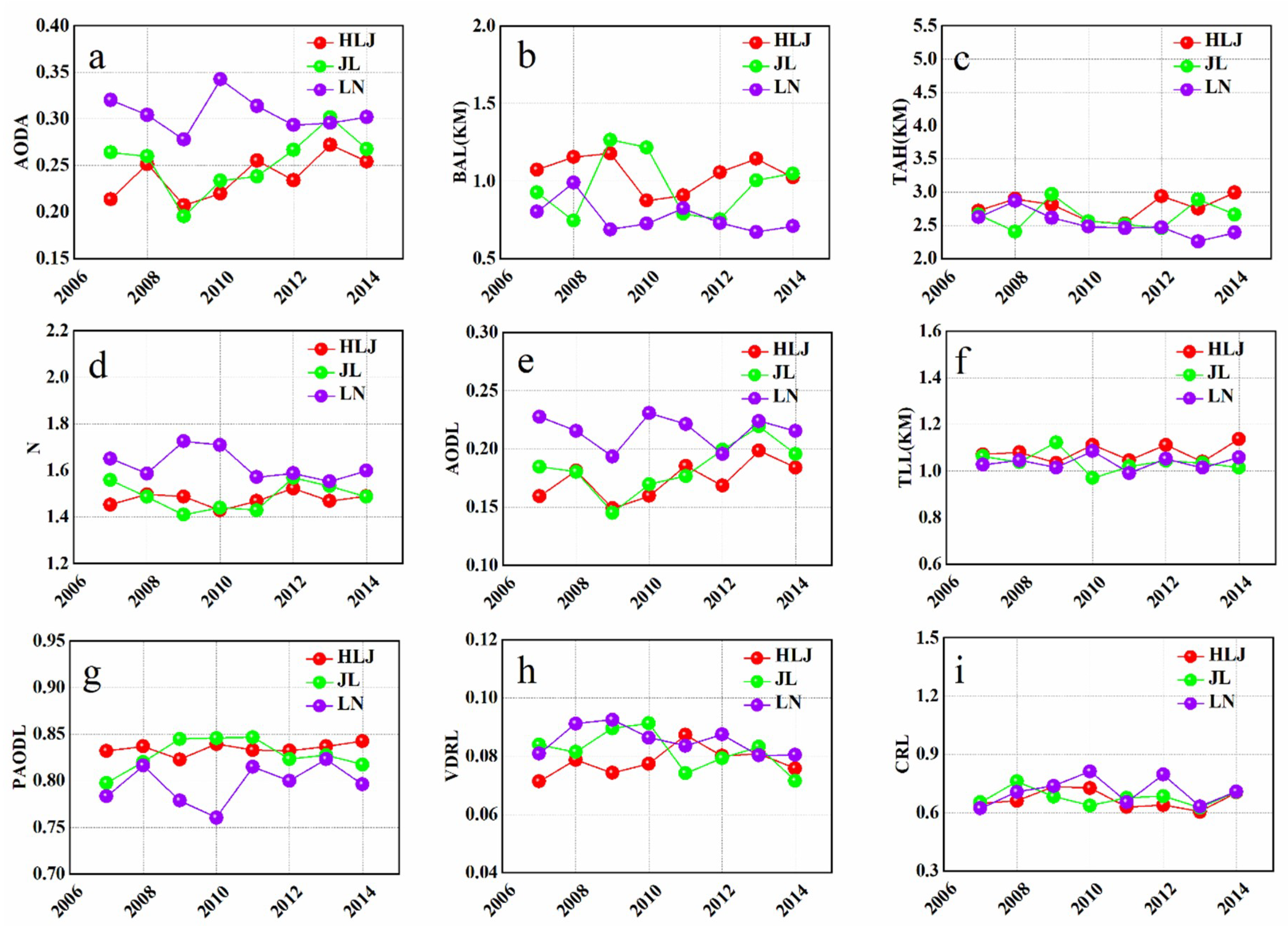
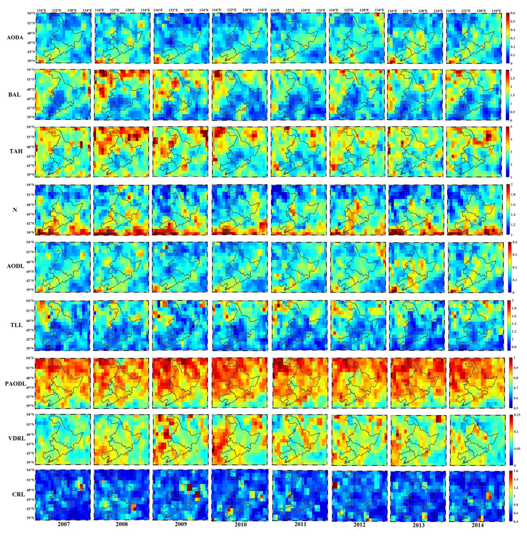
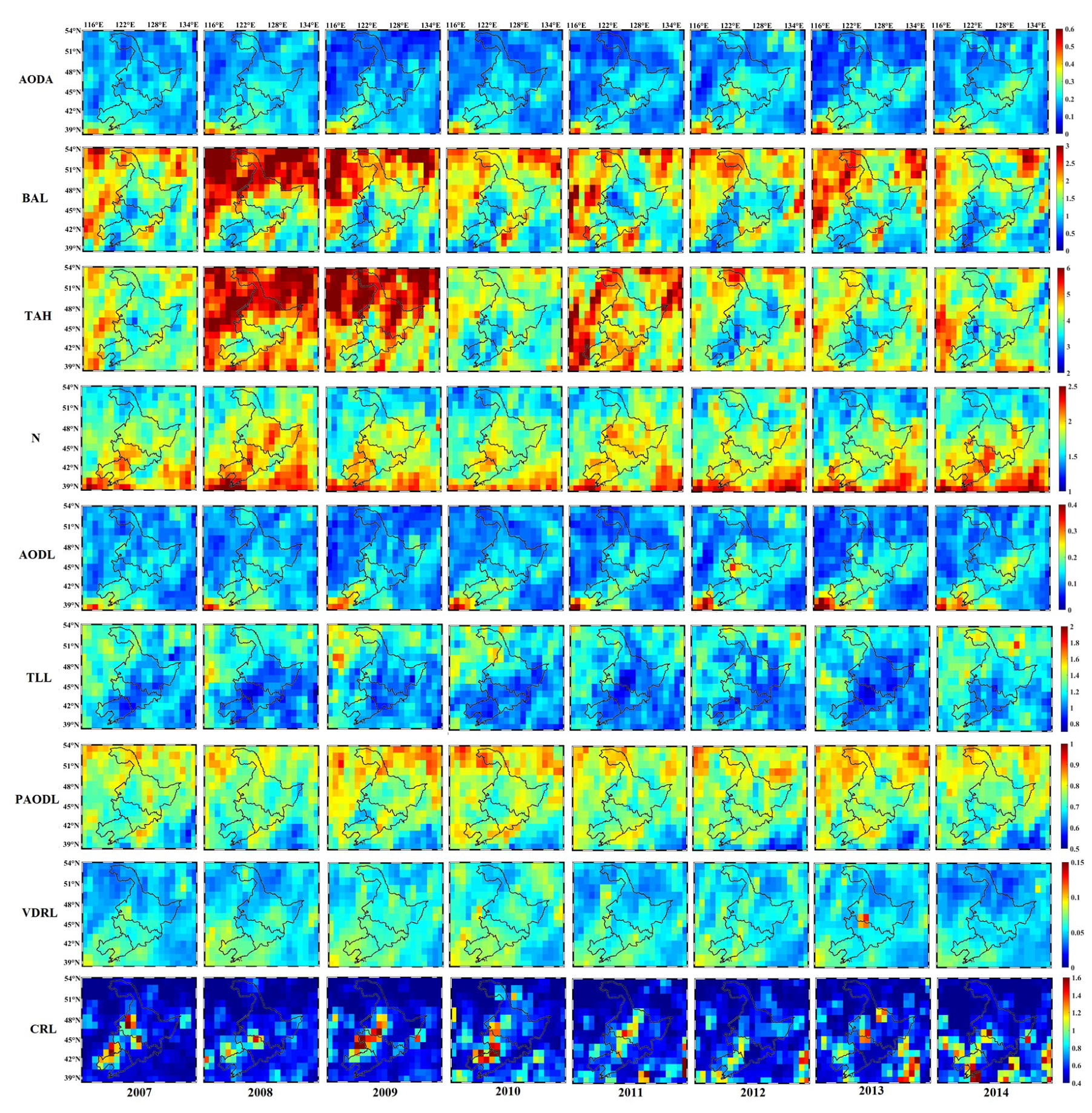
3.1. Inter-Annual Variation Characteristics of Aerosol Layers over NEC

Annual mean values of AODA were analyzed over NEC HLJ, JL, and LN (Figure 2a and Figure 3a). During each year (from 2007 to 2014), the annual mean AODA were the highest over LN (day: 0.27 to 0.35, night: 0.25 to 0.30) followed by JL (day: 0.20 to 0.30, night: 0.18 to 0.25) and HLJ (day: 0.20 to 0.27, night: 0.17 to 0.22). It can be seen from the spatial distribution maps (Figure 4 and Figure 5) that there is a banded high-value center in the annual mean AODA distribution, which is mainly composed of Dalian, Shenyang, Changchun, and Harbin cities, and runs from northeast to southwest. The banded high-value range keeps expanding and increasing year by year. This may be related to the topography and economic development of NEC. The area is surrounded by mountains on three sides and has a plain in the middle. Of the provinces studied, LN is close to the Beijing-Tianjin-Hebei region and, therefore, has a comparable level of industry and economic activity. Therefore, pollutant emissions are relatively large, resulting in high AODA values [33,38]. At the same time, from 2007 to 2014, the urban scale within JL and HLJ has increasingly witnessed an increase in human activities, and accentuated vehicle exhaust pollution, resulting in the increase of aerosol emissions in these two regions, accompanied by an expanding trend in annual mean AODA values. Moreover, the AODA annual mean values are higher during the day than at night, which might be caused by the larger number of pollutants discharged into the atmosphere by anthropogenic activities during the day than night [31].

The CALIOP aerosol layer data provides the top and base altitudes of each aerosol layer. We studied the base altitude of the lowest aerosol layer (BAL) and the top altitude of the highest aerosol layer (TAH). Figure 2b and Figure 3b show that the annual mean values of BAL are similar in the three regions (day 0.2 to 1.3, night 0.8 to 1.8). In terms of spatial distribution (Figure 4 and Figure 5), the BAL has a relatively high correlation with the topography, i.e., low values on the plain area and high values in mountainous areas. Similarly, the TAH values also showed a greater correlation with the topography (Figure 2c and Figure 3c, Figure 4 and Figure 5). These results are also similar to a study on the Yellow River Basin [39,40]. In general, the BAL and TAH values in HLJ are slightly higher than those of the other two regions, and values for the mountainous area are higher than those for the plains.

Figure 2d and Figure 3d depict that the values of N were high over the LN (daytime: 1.6 to 1.8, evening: 1.9 to 2.2) compared to JL (day: 1.4 to 1.6, night: 1.7 to 1.9) and HLJ (day: 1.4 to 1.6, night: 1.7 to 1.9). A plausible reason could be that LN is located in the southernmost part of the three regions and belongs to the temperate continental monsoon climate. The temperature is relatively high; the atmospheric vertical motion is relatively strong; and the atmospheric aerosol loadings are relatively large, which might lead to stronger aerosol vertical stratification in the atmosphere [14,41]. Moreover, the spatial distribution of the annual mean values of N shows that values were higher over the Liao River Plain, Songnen Plain, and Sanjiang Plain, while values in the surrounding mountains are lower (Figure 4 and Figure 5). This might be due to the lower temperature, lower atmospheric convection, and lower atmospheric aerosol loadings in mountainous regions, compared with plain regions, resulting in weak, relatively vertical stratification of the atmosphere.

AODL is the AOD of the lowest aerosol layer and is strongly related to human activities [39,42]. Annual mean values of AODL (Figure 2d and Figure 3d) present a similar space-time variation with AODA, and values of LN (day: 0.20 to 0.25, night: 0.1 to 0.22) are still higher than those for JL (day: 0.15 to 0.22, night: 0.13 to 0.18) and HLJ (day: 0.15 to 0.2, night: 0.12 to 0.16). The values of TLL in three regions had no significant difference: 0.9 to 1.1 for daytime, and 0.9 to 1.2 for nighttime. PAODL represents the proportion of AODL in AODA and the values of the three regions are not significantly different (day: 0.75 to 0.85, night: 0.77 to 0.8), being higher in the daytime than at nighttime. This revealed that aerosols are mainly concentrated in the lowest atmospheric layers. In the overall spatial distribution results (Figure 4 and Figure 5), the PAODL values are higher over the mountains and lower over the plains, which show that the lowest aerosol layers mostly occur due to weak vertical convection and atmospheric stratification [43,44].

The aerosol volume depolarization ratio (VDR) is the ratio of the vertical depolarization backscatter coefficient of 532 nm aerosol to the parallel depolarization backscatter coefficient of 532 nm, and it reflects the nonspherical properties of aerosols. The smaller the depolarization ratio value, the more spherical the shape of the aerosol particles. The annual mean values of VDRL (Figure 2h and Figure 3h) over LN (day: 0.08 to 0.10, night: 0.06 to 0.08) and JL (day: 0.07 to 0.09, night: 0.04 to 0.07) are slightly higher than those for HLJ (day: 0.06 to 0.09, night: 0.04 to 0.06), which might be because LN and JL are dominated by heavy industry, leading to significant nonspherical effects of aerosol emissions; the VDRL values are relatively high [42,45]. The spatial distribution maps in Figure 4h and Figure 5h show that the VDRL values are also relatively high (day ~0.15, night ~0.1) in western NEC (the Mongolian pastoral area) because this region often experiences sand dust in its atmosphere. Moreover, the VDRL values are higher during the day than during the night, which could be attributed to the increase of nonspherical particles in the atmosphere, caused by various human activities during the day. Figure 2i and Figure 3i show the annual mean variation of the aerosol color ratio of the lowest layer (CRL) over the three regions of NEC. The CRL reflects the size of the aerosol particles. The higher the CRL, the larger the aerosol particle size [13,39,42,43]. The CRL values of the three regions are not significantly different (day 0.6 to 0.9, night 0.5 to 0.8) and the CRL values are slightly higher in the daytime than at night, which might be due to decreased aerosol loadings due to sedimentation at night.

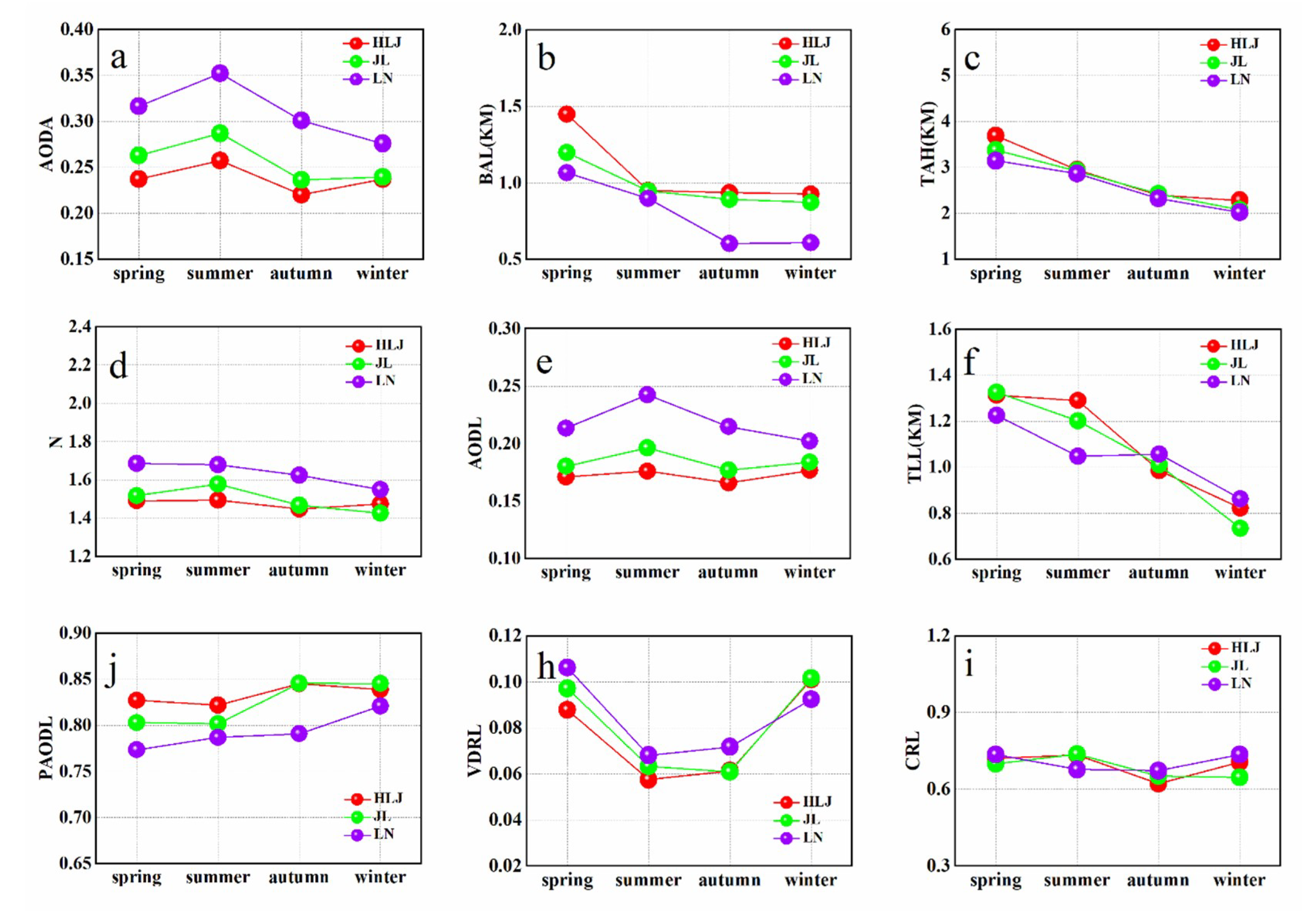
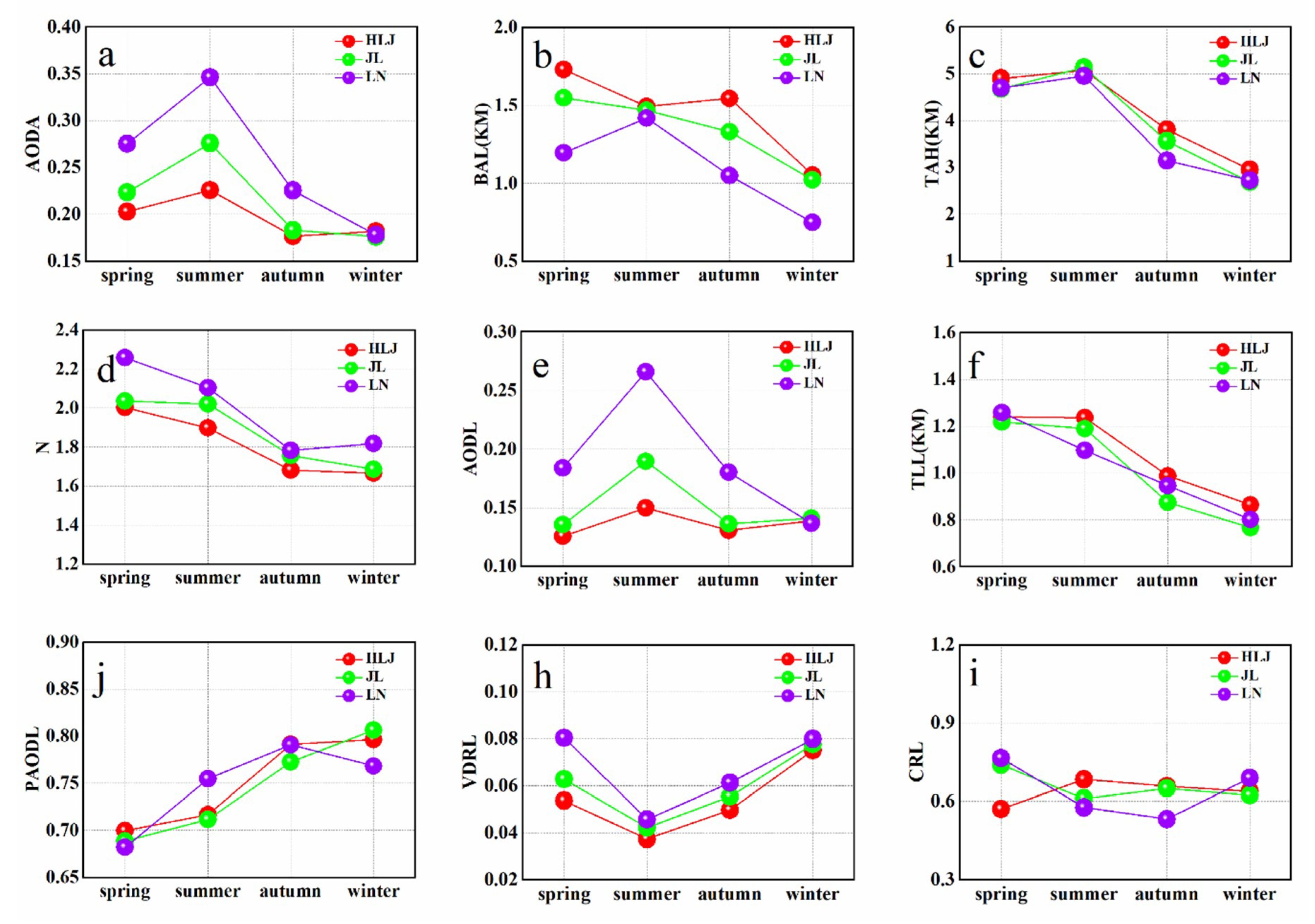
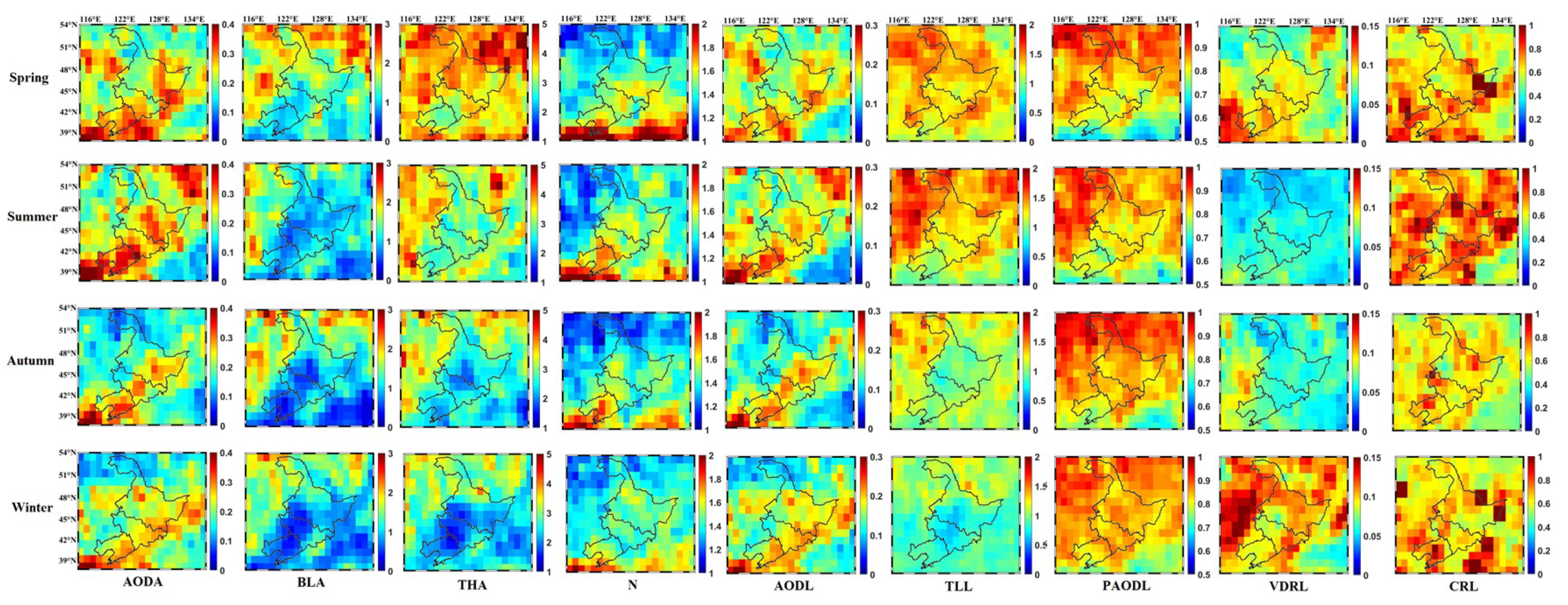
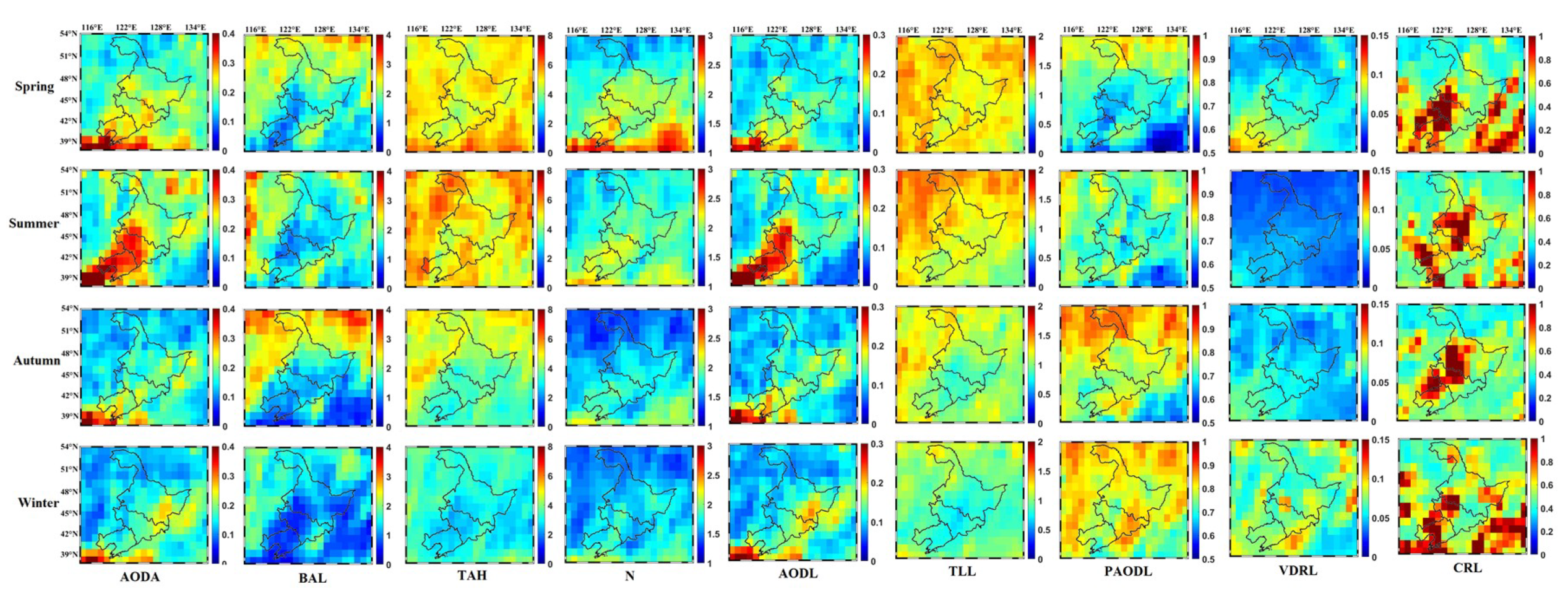
3.2. Seasonal Variation Characteristics of Aerosol Layers over NEC

Seasonal variations in AODA were also analyzed over the three provinces of NEC (Figure 6a, Figure 7a, Figure 8 and Figure 9, and

Table 1. Seasonal mean and standard deviation values of nine variables in the daytime over NEC (HLJ, JL, and LN).

Variables	Spring			Summer			Autumn			Winter
	HLJ/JL/LN			HLJ/JL/LN			HLJ/JL/LN			HLJ/JL/LN
AODA	0.24 ± 0.31	0.26 ± 0.29	0.32 ± 0.36	0.26 ± 0.33	0.29 ± 0.31	0.35 ± 0.37	0.22 ± 0.29	0.24 ± 0.30	0.30 ± 0.35	0.23 ± 0.32	0.24 ± 0.30	0.28 ± 0.34
BAL (km)	1.45 ± 1.72	1.20 ± 1.41	1.07 ± 1.44	0.95 ± 1.28	0.95 ± 1.10	0.90 ± 1.11	0.93 ± 1.34	0.89 ± 1.12	0.60 ± 0.83	0.93 ± 1.17	0.87 ± 1.01	0.61 ± 0.96
TAH (km)	3.69 ± 2.97	3.37 ± 2.72	3.15 ± 2.01	2.94 ± 2.23	2.92 ± 2.31	2.86 ± 2.55	2.39 ± 1.79	2.43 ± 1.99	2.32 ± 1.49	2.28 ± 1.95	2.07 ± 2.14	2.02 ± 1.63
N	1.49 ± 0.70	1.52 ± 0.67	1.69 ± 0.84	1.50 ± 0.72	1.58 ± 0.75	1.68 ± 0.82	1.45 ± 0.69	1.47 ± 0.68	1.63 ± 0.78	1.48 ± 0.69	1.43 ± 0.66	1.55 ± 0.77
AODL	0.17 ± 0.22	0.18 ± 0.21	0.21 ± 0.25	0.18 ± 0.21	0.20 ± 0.22	0.24 ± 0.26	0.17 ± 0.23	0.18 ± 0.23	0.21 ± 0.27	0.18 ± 0.25	0.18 ± 0.24	0.20 ± 0.26
TLL (km)	1.31 ± 0.82	1.33 ± 0.74	1.23 ± 0.78	1.29 ± 0.73	1.20 ± 0.67	1.05 ± 0.64	0.99 ± 0.63	1.01 ± 0.59	1.06 ± 0.54	0.82 ± 0.63	0.74 ± 0.46	0.86 ± 0.52
PAODL	0.83 ± 0.27	0.80 ± 0.28	0.77 ± 0.29	0.82 ± 0.27	0.80 ± 0.28	0.79 ± 0.28	0.85 ± 0.25	0.85 ± 0.25	0.79 ± 0.28	0.84 ± 0.26	0.85 ± 0.25	0.82 ± 0.27
VDRL	0.09 ± 0.09	0.10 ± 0.07	0.11 ± 0.08	0.06 ± 0.05	0.06 ± 0.05	0.07 ± 0.05	0.06 ± 0.06	0.06 ± 0.05	0.07 ± 0.05	0.10 ± 0.10	0.10 ± 0.26	0.09 ± 0.08
CRL	0.72 ± 1.45	0.70 ± 0.74	0.74 ± 0.65	0.73 ± 0.75	0.74 ± 0.54	0.68 ± 0.41	0.62 ± 0.70	0.65 ± 0.84	0.67 ± 0.90	0.71 ± 2.86	0.65 ± 1.15	0.74 ± 1.66

and

Table 2. Seasonal mean and standard deviation values of nine variables in the nighttime over NEC (HLJ, JL, and LN).

Variables	Spring			Summer			Autumn			Winter
	HLJ/JL/LN			HLJ/JL/LN			HLJ/JL/LN			HLJ/JL/LN
AODA	0.20 ± 0.32	0.22 ± 0.32	0.28 ± 0.36	0.23 ± 0.34	0.28 ± 0.35	0.35 ± 0.43	0.18 ± 0.30	0.18 ± 0.31	0.23 ± 0.38	0.18 ± 0.31	0.18 ± 0.28	0.18 ± 0.27
BAL (km)	1.73 ± 2.10	1.55 ± 1.97	1.20 ± 1.70	1.49 ± 2.32	1.47 ± 2.25	1.42 ± 2.39	1.54 ± 2.25	1.33 ± 1.84	1.05 ± 1.58	1.05 ± 1.53	1.02 ± 1.42	0.75 ± 1.18
TAH (km)	4.90 ± 2.56	4.68 ± 2.61	4.70 ± 2.61	5.07 ± 4.10	5.14 ± 4.15	4.95 ± 3.97	3.81 ± 3.03	3.57 ± 2.69	3.15 ± 2.33	2.95 ± 2.13	2.69 ± 2.02	2.73 ± 2.03
N	2.00 ± 1.06	2.04 ± 1.02	2.26 ± 1.14	1.90 ± 0.95	2.02 ± 1.03	2.10 ± 1.05	1.68 ± 0.86	1.76 ± 0.91	1.78 ± 0.87	1.67 ± 0.83	1.69 ± 0.82	1.82 ± 0.87
AODL	0.13 ± 0.24	0.14 ± 0.24	0.18 ± 0.30	0.15 ± 0.27	0.19 ± 0.30	0.27 ± 0.38	0.13 ± 0.25	0.14 ± 027	0.18 ± 0.34	0.14 ± 0.27	0.14 ± 0.25	0.14 ± 0.24
TLL (km)	1.24 ± 0.90	1.22 ± 0.90	1.26 ± 1.01	1.24 ± 0.84	1.19 ± 0.85	1.10 ± 0.77	0.99 ± 0.72	0.88 ± 0.61	0.95 ± 0.66	0.87 ± 0.68	0.77 ± 0.58	0.80 ± 0.60
PAODL	0.70 ± 0.32	0.69 ± 0.33	0.68 ± 0.32	0.72 ± 0.33	0.71 ± 0.33	0.75 ± 0.29	0.79 ± 0.29	0.77 ± 0.30	0.79 ± 0.28	0.80 ± 0.29	0.81 ± 0.27	0.77 ± 0.29
VDRL	0.05 ± 0.06	0.06 ± 0.06	0.08 ± 0.05	0.04 ± 0.03	0.04 ± 0.03	0.05 ± 0.03	0.05 ± 0.06	0.06 ± 0.05	0.06 ± 0.04	0.07 ± 0.14	0.08 ± 0.12	0.08 ± 0.07
CRL	0.57 ± 1.54	0.74 ± 2.96	0.77 ± 2.96	0.68 ± 1.90	0.61 ± 1.85	0.58 ± 1.85	0.66 ± 2.36	0.65 ± 1.88	0.53 ± 1.88	0.64 ± 1.94	0.62 ± 2.01	0.69 ± 2.01

). The AODA values increased from spring (day: 0.24 to 0.32, night: 0.20 to 0.28) to summer (day: 0.26 to 0.35, night: 0.23 to 0.35) and decreased in autumn (day: 0.22 to 0.30, night: 0.18 to 0.23) over the whole NEC. In July, the monthly average was the highest during the day (HLJ 0.33, JL 0.36, and LN 0.41), see

Table 3. Monthly mean and standard deviation values of nine variables in the daytime over NEC (HLJ, JL, and LN). For each variable, the top row is the value over HLJ, the middle row is the value over JL, and the bottom row is the value over LN.

Variables	Jan	Feb	Mar	Apr	May	Jun	Jul	Aug	Sep	Oct	Nov	Dec
	M/σ	M/σ	M/σ	M/σ	M/σ	M/σ	M/σ	M/σ	M/σ	M/σ	M/σ	M/σ
AODA	0.23 ± 0.29	0.25 ± 0.31	0.27 ± 0.35	0.26 ± 0.27	0.18 ± 0.19	0.23 ± 0.25	0.33 ± 0.39	0.20 ± 0.20	0.16 ± 0.19	0.27 ± 0.30	0.21 ± 0.28	0.23 ± 0.31
	0.25 ± 0.28	0.28 ± 0.29	0.30 ± 0.33	0.27 ± 0.25	0.22 ± 0.21	0.26 ± 0.23	0.36 ± 0.34	0.21 ± 0.22	0.20 ± 0.19	0.29 ± 0.35	0.20 ± 0.22	0.23 ± 0.30
	0.29 ± 0.33	0.28 ± 0.31	0.27 ± 0.31	0.34 ± 0.31	0.32 ± 0.33	0.31 ± 0.29	0.41 ± 0.38	0.36 ± 0.35	0.31 ± 0.34	0.32 ± 0.33	0.27 ± 0.33	0.28 ± 0.34
BAL	0.81 ± 1.03	0.95 ± 1.14	1.361.34	1.34 ± 1.65	1.56 ± 1.73	1.05 ± 1.26	0.84 ± 0.98	0.98 ± 1.28	1.15 ± 1.48	0.871.07	0.911.23	1.051.25
	0.78 ± 0.74	0.75 ± 0.70	1.41 ± 1.35	1.01 ± 1.04	1.24 ± 1.39	0.91 ± 0.74	1.02 ± 0.95	0.97 ± 1.14	0.98 ± 1.09	0.94 ± 1.03	0.84 ± 0.86	1.00 ± 0.94
	0.61 ± 0.89	0.65 ± 0.96	0.84 ± 0.91	0.98 ± 1.31	1.33 ± 1.54	1.03 ± 1.02	1.04 ± 0.92	0.70 ± 0.92	0.68 ± 0.84	0.61 ± 0.75	0.61 ± 0.85	0.59 ± 0.77
TAH	2.03 ± 1.74	2.30 ± 1.78	3.63 ± 3.39	3.58 ± 2.58	3.62 ± 1.91	3.22 ± 1.70	2.77 ± 1.96	2.76 ± 1.99	3.07 ± 2.00	2.40 ± 1.50	2.05 ± 1.55	2.51 ± 1.86
	2.00 ± 1.79	2.22 ± 1.98	3.29 ± 2.35	3.17 ± 1.87	3.57 ± 2.19	3.21 ± 1.74	3.00 ± 1.84	2.54 ± 1.23	2.71 ± 1.52	2.59 ± 1.49	2.06 ± 1.77	2.05 ± 1.24
	2.12 ± 1.42	2.09 ± 1.62	2.45 ± 1.56	3.20 ± 1.31	3.63 ± 1.83	3.14 ± 1.99	2.96 ± 2.37	2.40 ± 1.59	2.64 ± 1.33	2.40 ± 1.56	2.09 ± 1.20	1.86 ± 1.05
N	1.42 ± 0.64	1.46 ± 0.60	1.44 ± 0.63	1.51 ± 0.66	1.47 ± 0.69	1.48 ± 0.66	1.54 ± 0.75	1.40 ± 0.59	1.38 ± 0.59	1.53 ± 0.69	1.38 ± 0.63	1.52 ± 0.68
	1.42 ± 0.62	1.43 ± 0.60	1.42 ± 0.63	1.55 ± 0.62	1.50 ± 0.65	1.71 ± 0.80	1.62 ± 0.73	1.40 ± 0.57	1.40 ± 0.59	1.56 ± 0.71	1.37 ± 0.57	1.44 ± 0.66
	1.66 ± 0.80	1.51 ± 0.71	1.50 ± 0.69	1.77 ± 0.87	1.78 ± 0.87	1.73 ± 0.73	1.65 ± 0.76	1.59 ± 0.75	1.64 ± 0.69	1.64 ± 0.73	1.58 ± 0.77	1.49 ± 0.64
AODL	0.18 ± 0.22	0.18 ± 0.23	0.20 ± 0.26	0.18 ± 0.20	0.14 ± 0.15	0.17 ± 0.18	0.21 ± 0.24	0.15 ± 0.14	0.12 ± 0.14	0.20 ± 0.25	0.17 ± 0.22	0.18 ± 0.25
	0.20 ± 0.23	0.21 ± 0.23	0.21 ± 0.22	0.19 ± 0.19	0.15 ± 0.16	0.17 ± 0.15	0.24 ± 0.23	0.16 ± 0.18	0.15 ± 0.14	0.21 ± 0.25	0.16 ± 0.18	0.17 ± 0.25
	0.20 ± 0.23	0.21 ± 0.24	0.19 ± 0.21	0.23 ± 0.24	0.21 ± 0.23	0.21 ± 0.20	0.30 ± 0.29	0.25 ± 0.26	0.22 ± 0.24	0.23 ± 0.27	0.20 ± 0.26	0.21 ± 0.27
TLL	0.75 ± 0.55	0.87 ± 0.60	1.14 ± 0.69	1.39 ± 0.81	1.34 ± 0.83	1.46 ± 0.80	1.22 ± 0.67	1.22 ± 0.65	1.24 ± 0.72	0.99 ± 0.59	0.83 ± 0.51	0.84 ± 0.65
	0.70 ± 0.43	0.80 ± 0.43	1.16 ± 0.63	1.42 ± 0.74	1.41 ± 0.72	1.30 ± 0.63	1.09 ± 0.60	1.17 ± 0.59	1.27 ± 0.70	1.06 ± 0.55	0.80 ± 0.37	0.71 ± 0.44
	0.80 ± 0.51	0.88 ± 0.44	1.01 ± 0.55	1.38 ± 0.83	1.29 ± 0.83	1.13 ± 0.71	0.88 ± 0.46	1.06 ± 0.57	1.15 ± 0.62	1.06 ± 0.46	0.94 ± 0.45	0.89 ± 0.47
PAODL	0.85 ± 0.24	0.84 ± 0.26	0.85 ± 0.25	0.81 ± 0.27	0.84 ± 0.25	0.83 ± 0.25	0.82 ± 0.27	0.84 ± 0.25	0.87 ± 0.22	0.83 ± 0.26	0.87 ± 0.23	0.84 ± 0.25
	0.85 ± 0.24	0.83 ± 0.24	0.84 ± 0.27	0.79 ± 0.28	0.81 ± 0.27	0.76 ± 0.29	0.79 ± 0.26	0.85 ± 0.25	0.87 ± 0.23	0.84 ± 0.24	0.86 ± 0.25	0.85 ± 0.24
	0.80 ± 0.27	0.83 ± 0.26	0.84 ± 0.25	0.74 ± 0.30	0.76 ± 0.30	0.78 ± 0.27	0.81 ± 0.24	0.81 ± 0.27	0.76 ± 0.29	0.79 ± 0.27	0.82 ± 0.26	0.84 ± 0.25
VDRL	0.09 ± 0.08	0.11 ± 0.10	0.11 ± 0.11	0.08 ± 0.08	0.07 ± 0.06	0.06 ± 0.04	0.06 ± 0.05	0.06 ± 0.06	0.06 ± 0.05	0.05 ± 0.04	0.07 ± 0.07	0.11 ± 0.09
	0.10 ± 0.10	0.11 ± 0.26	0.11 ± 0.09	0.09 ± 0.06	0.09 ± 0.06	0.06 ± 0.04	0.06 ± 0.05	0.06 ± 0.04	0.07 ± 0.04	0.06 ± 0.04	0.06 ± 0.06	0.10 ± 0.10
	0.08 ± 0.06	0.09 ± 0.07	0.11 ± 0.08	0.10 ± 0.06	0.11 ± 0.07	0.07 ± 0.04	0.06 ± 0.04	0.07 ± 0.05	0.07 ± 0.05	0.07 ± 0.04	0.07 ± 0.05	0.11 ± 0.09
CRL	0.60 ± 0.44	0.64 ± 0.49	0.68 ± 0.60	0.81 ± 1.46	0.65 ± 0.40	0.71 ± 0.56	0.73 ± 0.44	0.77 ± 0.75	0.68 ± 0.48	0.58 ± 0.44	0.59 ± 0.64	0.80 ± 1.87
	0.76 ± 1.27	0.64 ± 0.40	0.72 ± 0.75	0.62 ± 0.27	0.71 ± 0.42	0.70 ± 0.30	0.78 ± 0.47	0.78 ± 0.57	0.73 ± 0.38	0.60 ± 0.52	0.65 ± 0.88	0.59 ± 0.35
	0.63 ± 0.42	0.91 ± 1.41	0.79 ± 0.70	0.77 ± 0.53	0.70 ± 0.38	0.68 ± 0.32	0.63 ± 0.34	0.70 ± 0.40	0.68 ± 0.38	0.77 ± 0.82	0.58 ± 0.46	0.65 ± 0.54

and

Table 4. Monthly mean and standard deviation values of nine variables in the nighttime over NEC (HLJ, JL, and LN). For each variable, the top row is the value over HLJ, the middle row is the value over JL, and the bottom row is the value over LN.

Variables	Jan	Feb	Mar	Apr	May	Jun	Jul	Aug	Sep	Oct	Nov	Dec
	M/σ	M/σ	M/σ	M/σ	M/σ	M/σ	M/σ	M/σ	M/σ	M/σ	M/σ	M/σ
AODA	0.18 ± 0.30	0.19 ± 0.30	0.17 ± 0.29	0.26 ± 0.35	0.18 ± 0.27	0.24 ± 0.31	0.23 ± 0.32	0.21 ± 0.32	0.14 ± 0.23	0.20 ± 0.32	0.18 ± 0.28	0.18 ± 0.31
	0.16 ± 0.23	0.17 ± 0.28	0.20 ± 0.30	0.27 ± 0.32	0.21 ± 0.29	0.31 ± 0.35	0.29 ± 0.33	0.23 ± 0.28	0.16 ± 0.25	0.21 ± 0.31	0.18 ± 0.29	0.20 ± 0.31
	0.17 ± 0.23	0.21 ± 0.31	0.28 ± 0.35	0.24 ± 0.33	0.31 ± 0.35	0.37 ± 0.44	0.37 ± 0.43	0.30 ± 0.36	0.25 ± 0.31	0.26 ± 0.42	0.17 ± 0.27	0.18 ± 0.25
BAL	1.05 ± 1.47	1.12 ± 1.58	1.54 ± 1.93	1.49 ± 1.86	2.17 ± 2.31	1.55 ± 2.11	1.48 ± 2.16	1.46 ± 2.01	1.72 ± 2.29	1.77 ± 2.30	1.19 ± 1.52	1.00 ± 1.41
	1.05 ± 1.32	1.05 ± 1.40	1.59 ± 2.01	1.25 ± 1.51	1.92 ± 2.13	1.67 ± 1.88	1.40 ± 2.18	1.35 ± 2.04	1.54 ± 1.95	1.41 ± 1.83	1.22 ± 1.34	1.00 ± 1.33
	0.70 ± 0.96	0.84 ± 1.23	1.10 ± 1.51	1.23 ± 1.68	1.26 ± 1.66	1.38 ± 1.77	1.70 ± 2.30	1.08 ± 1.67	1.22 ± 1.57	1.05 ± 1.55	1.00 ± 1.23	0.74 ± 1.08
TAH	2.78 ± 2.04	3.41 ± 2.14	4.16 ± 2.34	4.95 ± 2.34	5.58 ± 2.55	4.79 ± 2.95	5.43 ± 3.36	4.64 ± 2.98	4.53 ± 3.16	4.01 ± 2.72	2.96 ± 2.22	2.67 ± 1.97
	2.81 ± 1.94	3.02 ± 1.96	3.99 ± 2.39	4.75 ± 2.29	5.33 ± 2.50	5.24 ± 2.72	5.38 ± 3.09	4.23 ± 2.94	4.48 ± 2.91	3.65 ± 2.24	2.81 ± 2.03	2.64 ± 1.81
	2.64 ± 1.95	3.03 ± 2.04	4.20 ± 2.23	4.84 ± 2.41	5.20 ± 2.46	5.46 ± 3.24	5.29 ± 3.23	3.92 ± 2.31	3.86 ± 2.45	3.09 ± 2.19	2.71 ± 1.87	2.58 ± 1.79
N	1.63 ± 0.83	1.78 ± 0.88	1.83 ± 0.92	2.16 ± 1.11	1.98 ± 1.02	1.92 ± 0.97	1.86 ± 0.89	1.86 ± 0.90	1.73 ± 0.86	1.71 ± 0.87	1.56 ± 0.75	1.58 ± 0.75
	1.69 ± 0.76	1.81 ± 0.87	1.84 ± 0.90	2.18 ± 1.00	2.05 ± 0.98	2.12 ± 1.06	1.99 ± 0.93	1.86 ± 0.89	1.83 ± 0.94	1.82 ± 0.88	1.57 ± 0.71	1.64 ± 0.77
	1.81 ± 0.88	1.88 ± 0.85	2.15 ± 0.97	2.24 ± 1.10	2.38 ± 1.17	2.16 ± 1.01	2.02 ± 0.97	2.05 ± 0.98	1.91 ± 0.95	1.77 ± 0.83	1.68 ± 0.75	1.77 ± 0.82
AODL	0.14 ± 0.26	0.14 ± 0.26	0.12 ± 0.23	0.16 ± 0.27	0.11 ± 0.20	0.15 ± 0.25	0.16 ± 0.27	0.14 ± 0.25	0.09 ± 0.18	0.15 ± 0.26	0.15 ± 0.24	0.15 ± 0.27
	0.12 ± 0.21	0.13 ± 0.24	0.14 ± 0.25	0.16 ± 0.23	0.12 ± 0.19	0.20 ± 0.28	0.22 ± 0.28	0.17 ± 0.23	0.10 ± 0.18	0.17 ± 0.27	0.15 ± 0.25	0.17 ± 0.28
	0.13 ± 0.19	0.15 ± 0.26	0.20 ± 0.31	0.16 ± 0.27	0.19 ± 0.28	0.27 ± 0.37	0.29 ± 0.38	0.24 ± 0.34	0.19 ± 0.26	0.21 ± 0.37	0.13 ± 0.23	0.15 ± 0.23
TLL	0.82 ± 0.65	0.94 ± 0.69	1.08 ± 0.75	1.29 ± 0.91	1.33 ± 0.95	1.37 ± 0.91	1.20 ± 0.77	1.12 ± 0.74	1.15 ± 0.82	0.96 ± 0.66	0.86 ± 0.61	0.84 ± 0.66
	0.76 ± 0.49	0.77 ± 0.54	1.11 ± 0.76	1.27 ± 0.91	1.28 ± 0.93	1.35 ± 0.99	1.15 ± 0.71	1.06 ± 0.64	1.01 ± 0.64	0.91 ± 0.62	0.74 ± 0.48	0.82 ± 0.63
	0.76 ± 0.54	0.83 ± 0.62	1.18 ± 0.80	1.34 ± 1.05	1.30 ± 1.07	1.16 ± 0.85	1.08 ± 0.66	1.02 ± 0.67	1.02 ± 0.62	1.02 ± 0.72	0.81 ± 0.54	0.83 ± 0.56
PAODL	0.82 ± 0.28	0.75 ± 0.31	0.74 ± 0.30	0.67 ± 0.33	0.69 ± 0.32	0.70 ± 0.32	0.74 ± 0.31	0.73 ± 0.31	0.74 ± 0.32	0.80 ± 0.29	0.84 ± 0.26	0.82 ± 0.27
	0.80 ± 0.25	0.76 ± 0.28	0.74 ± 0.30	0.66 ± 0.32	0.68 ± 0.32	0.68 ± 0.33	0.74 ± 0.31	0.74 ± 0.31	0.72 ± 0.32	0.77 ± 0.29	0.84 ± 0.24	0.84 ± 0.24
	0.77 ± 0.28	0.74 ± 0.29	0.70 ± 0.30	0.69 ± 0.31	0.66 ± 0.33	0.73 ± 0.30	0.78 ± 0.27	0.77 ± 0.28	0.76 ± 0.29	0.80 ± 0.28	0.81 ± 0.26	0.80 ± 0.26
VDRL	0.07 ± 0.13	0.07 ± 0.12	0.06 ± 0.07	0.05 ± 0.05	0.05 ± 0.05	0.04 ± 0.03	0.03 ± 0.03	0.04 ± 0.03	0.05 ± 0.03	0.04 ± 0.04	0.06 ± 0.08	0.08 ± 0.11
	0.07 ± 0.11	0.08 ± 0.12	0.06 ± 0.06	0.06 ± 0.05	0.07 ± 0.05	0.04 ± 0.03	0.04 ± 0.03	0.04 ± 0.03	0.05 ± 0.03	0.05 ± 0.04	0.06 ± 0.06	0.08 ± 0.08
	0.07 ± 0.05	0.09 ± 0.08	0.08 ± 0.06	0.08 ± 0.04	0.08 ± 0.05	0.05 ± 0.03	0.05 ± 0.03	0.04 ± 0.03	0.05 ± 0.03	0.06 ± 0.03	0.07 ± 0.05	0.09 ± 0.07
CRL	0.59 ± 1.61	0.61 ± 1.37	0.59 ± 1.55	0.58 ± 1.33	0.53 ± 0.75	0.65 ± 1.12	0.73 ± 1.69	0.66 ± 1.70	0.75 ± 2.00	0.64 ± 1.92	0.62 ± 1.81	0.69 ± 2.02
	0.63 ± 1.56	0.62 ± 1.40	0.60 ± 1.32	0.70 ± 1.80	0.92 ± 2.43	0.58 ± 0.71	0.68 ± 1.47	0.54 ± 0.60	0.57 ± 0.88	0.66 ± 1.36	0.63 ± 1.28	0.65 ± 1.49
	0.62 ± 1.22	0.75 ± 1.71	0.79 ± 1.85	0.69 ± 1.14	0.81 ± 2.06	0.53 ± 0.46	0.55 ± 0.67	0.63 ± 1.06	0.54 ± 0.60	0.50 ± 0.54	0.55 ± 0.88	0.76 ± 1.53

. In terms of spatial variation, during spring and summer, the AODA values decreased gradually from southwest to northeast NEC. In autumn and winter, the high AODA values appeared in the middle parts of LN and JL. NEC belongs to a continental monsoon climate with less precipitation and more sandy weather in spring. Some studies have pointed out that high AOD values have a good correlation with dust aerosols during frequently dusty weather [46,47], resulting in high AOD values in spring. Moreover, the AODA values are higher in summer than spring, which might also be related to the increase of relative humidity in summer [48,49]. The increase in relative humidity will promote the growth of aerosol hygroscopicity and the transformation of gas particles, thus increasing the aerosol AOD values. The air in autumn is relatively dry and, under the influence of a monsoon climate, causing the pollutants to diffuse and settle quickly; the overall air quality is relatively high, resulting in the decline of AODA values in summer [31,32,33]. Moreover, the AODA values are higher in the daytime than at night, which is mainly due to the release of various pollutants into the atmosphere by various anthropogenic activities in the daytime.

Figure 6b and Figure 7b and Table 1 and Table 2 illustrate that the BAL seasonal mean values are higher in spring and summer (day: 0.9 to 1.5, night: 1.2 to 1.7) than in autumn and winter (day: 0.6 to 0.9, night: 0.8 to 1.5) for the entire NEC. As can be seen from Table 3 and Table 4, the monthly average is highest in May. This might be because the temperature in spring and summer is higher than that in autumn and winter, and the vertical convection is correspondingly stronger, resulting in increasing BAL values. The BAL values for HLJ (day: 0.9 to 1.5, night: 1.1 to 1.7) are slightly higher than JL (day: 0.9 to 1.2, night: 1.0 to 1.6) and LN (day: 0.6 to 1.1, night: 0.8 to 1.4), which might be due to topography. From the spatial distribution maps (Figure 8 and Figure 9), it can also be seen that the BAL values are lower in plain areas (day ~1, night ~2), whereas higher in mountain areas (day ~2, night ~3). The TAH seasonal mean values vary little across the NEC. The results depict a decreasing seasonal trend from spring and summer (day: 3 to 4, night: 4 to 5) to autumn and winter (day: 2 to 3, night: 3 to 4). The trends of the TAH values are similar to the BAL variation, which is probably due to the enhancement of vertical convection, caused by seasonal temperature, resulting in the heightening of the lowest aerosol layer [49,50]. On the other hand, straw burning is often carried out in the spring and summer, which could lead to an increase in aerosol emissions and TAH values [51,52].

The seasonal mean values of N over the three provinces exhibit a gradual decline from spring; the monthly average being highest in April (evening value of 2.16), followed by summer, autumn, and then winter. Spring values for LN (day ~2.2, night ~2.6) are much higher than for the other two regions. The results might be caused by high temperatures and strong vertical convection in spring, leading to obvious aerosol stratification [44]. Overall, the values for LN (day: 1.5 to 1.7, night: 1.8 to 2.3) are slightly higher than JL (day: 1.4 to 1.6, night: 1.7 to 2.0) and HLJ (day: 1.4 to 1.5, night: 1.7 to 2.0). Figure 8 and Figure 9 demonstrate that high N values are mainly concentrated in central LN and JL. Such high values can be attributed to two plausible reasons: Firstly, this region comprises a largely plain terrain and has a developed economy with pronounced daily industrial production, automobile exhausts, and other pollutant emissions are high; secondly, this region experiences the temperate monsoon climate and the vertical movement of the air is strong, resulting in obvious vertical stratification of the atmosphere and, hence, increased aerosol stratification [34,35].

The seasonal variation of AODL values is similar to their variation in time and space distribution over the NEC. The seasonal mean values of TLL are largest in spring, followed by summer, autumn, and winter. This might explain the dry air and dusty weather in the spring. Moreover, the TLL values in the daytime are higher than those in the evening, plausibly affected by human activities, such as industries and other life-sustaining functions [40,53,54]. The seasonal mean values of PAODL generally increased from spring and summer (day: 0.75 to 0.83, night: 0.65 to 0.75) to autumn and winter (day: 0.80 to 0.85, night: 0.75 to 0.80), which might be related to the magnitude of the N values discussed earlier [44,55,56]. The N values from spring and summer are larger than those from autumn and winter, following the pattern that the values of PAODL increase from spring and summer (0.77 to 0.83 during the day, 0.67 to 0.75 at night) to autumn and winter (day: 0.80 to 0.85, night: 0.76 to 0.80). From the spatial distribution map, it can also be seen that PAODL has a certain correlation with N. The larger the N values, the smaller the PAODL values. In addition, the PAODL values are higher during the day than at night, which might be the reason why the lowest layers of aerosols are dominated by dust [38,39]. Needless to state that during the day, human activities are conventionally rather frequent, which results in higher PAODL values.

The seasonal mean values of VDRL are higher in spring and winter (day: 0.09 to 0.11, night: 0.05 to 0.08) than in summer and autumn (day: 0.06 to 0.07, night: 0.04 to 0.06), which might be caused by the relatively severe dust events in these two seasons, resulting in the atmospheric characteristics seen in the lowest aerosol layers. The VDRL values for LN are slightly higher than JL and HLJ, probably related to the level of economic development and specific industry types, resulting in higher contents of sand aerosols in LN and, thus, a larger VDRL value. The seasonal mean values of VDRL are higher during the day than at night, which could be caused by various industrial activities during the day, and also pollutants released by automobile exhausts [47,48]. The value of CRL did not change significantly with the seasons, however, the difference between day and night in autumn and winter are found higher than the difference in spring and summer; this may be caused by the cold autumn and winter in NEC, leading to the heavy use of coal-powered heating at night and, therefore, the discharge of pollutants into the atmosphere [19,20].

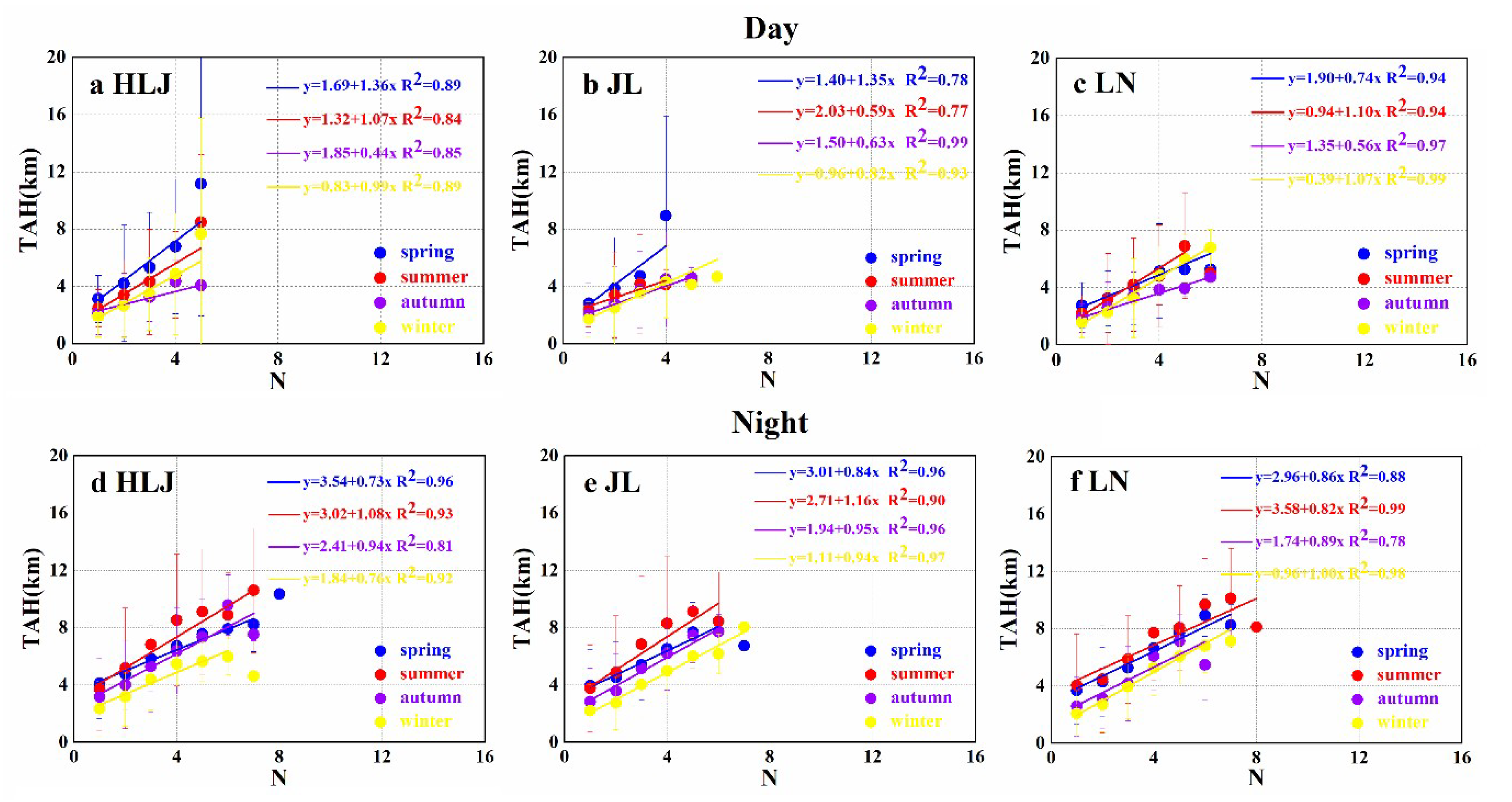
3.3. The Correlation of Aerosol Properties over NEC

To better appreciate the temporal and spatial distribution characteristics of aerosols over NEC, we studied the correlations among the aerosol parameters of HLJ, JL, and LN in the spring, summer, autumn, and winter. The correlation between AODL and TLL in these three regions is shown in Figure 10. The relationship between AODL and TLL reflects the aerosol concentrations to some extent. If the correlation between AODL and TLL is strong, it signifies high aerosol loadings [33,39]. Figure 10 demonstrates that the TLL and AODL over the three regions have a weak, positive correlation, but not so significant (R² < 0.5), indicating that the aerosol concentration is not substantial. For all the four seasons, the three regions have the highest correlation in winter, which might be due to the winter coal-fueled heating and burning of gas in NEC. Consequently, pollutants emitted into the atmosphere relatively enhance the aerosol concentration in its bottom layer.

Figure 11 depicts that TAH has a strong positive correlation with N. That is, the larger the values of N, the greater the values of TAH. This is consistent with the logical presumption that the more the aerosol layers (N), the thicker the atmosphere, resulting in higher TAH. These results are also similar to the results reported by studies of the Tibetan Plateau [39] and the Yellow River Basin [33].

Figure 12 reveals a negative correlation between PAODL and N over the three provinces: The larger the value of N, the smaller the PAODL. This is because PAODL represents the proportion of AODL in AODA. These results are also similar to the results by [39] and [33].

Figure 13 exhibits the scatter distribution graph between VDRL and CRL over NEC (HLJ, JL, and LN). It can be seen that most of the scattered points are in the range of CRL 0–1 and VDRL 0–1, being particularly concentrated in the range for VDRL: 0.0 to 0.2 and CRL: 0.5 to 1.0. This indicates that, in the lowest aerosol layer over NEC, the particle sizes are smaller with nonspherical shapes. The values of VDRL in HLJ are more dispersed than those in LN and JL, however, the average is slightly smaller. Compared with JL and HLJ, CRL and VDRL in LN are more concentrated and smaller. This might be due to the higher levels of pollution in LN, where pollutant particles tend to be smaller and nonspherical. Moreover, there are rather large CRL values at night than during the day, probably due to the residual large aerosol particles being transported to higher altitudes during the nighttime.

4. Conclusions

The optical and physical properties of the aerosol layers over Northeast China (NEC) have been investigated in this study using CALIPSO Level 2 layer products, from 2007 to 2014. The inter-annual and seasonal variations of AODA, BAL, TAH, N, AODL, TLL, PAODL, VDRL, and CRL during day and night are expressly examined. The main conclusions are:

• Relatively large values of AODA are observed over the LN province, as LN hosts a robust industrial economy and, thereby, experiences extreme pollution. Seasonally, the values of AODA rose from spring to summer and decreased in autumn, which is caused by NEC’s temperate monsoon climate. Moreover, due to industrial units and various anthropogenic activities in the daytime, the AOD values are higher than that in the nighttime.
• The values of BAH and TAH demonstrate a correlation with topography. Moreover, higher BAH and TAH values are observed in the spring and summer compared to autumn and winter.
• High values of N are observed over LN. N values gradually decreased from spring to summer to autumn and winter. This might be due to the influence of the temperate monsoon climate, where the vertical movement of the atmospheric constituents is characteristically stronger in spring, leading to a significant vertical stratification of the atmosphere.
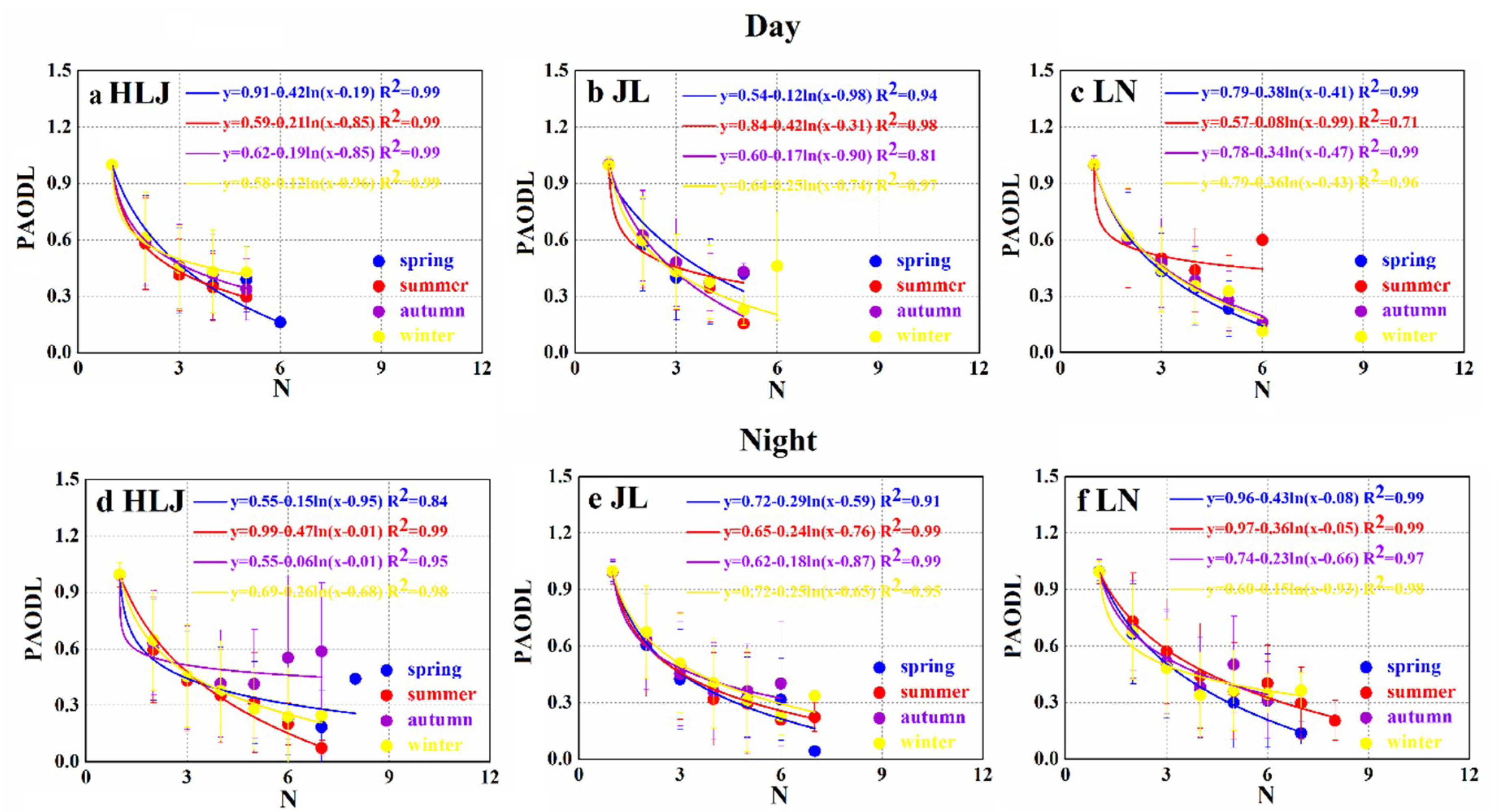
• The values of TLL and PAODL in the three provinces are not significantly different from each other. The values in the daytime are higher than that in the evening, which might be induced by high aerosol concentrations in the bottom layer from anthropogenic activities in the daytime.
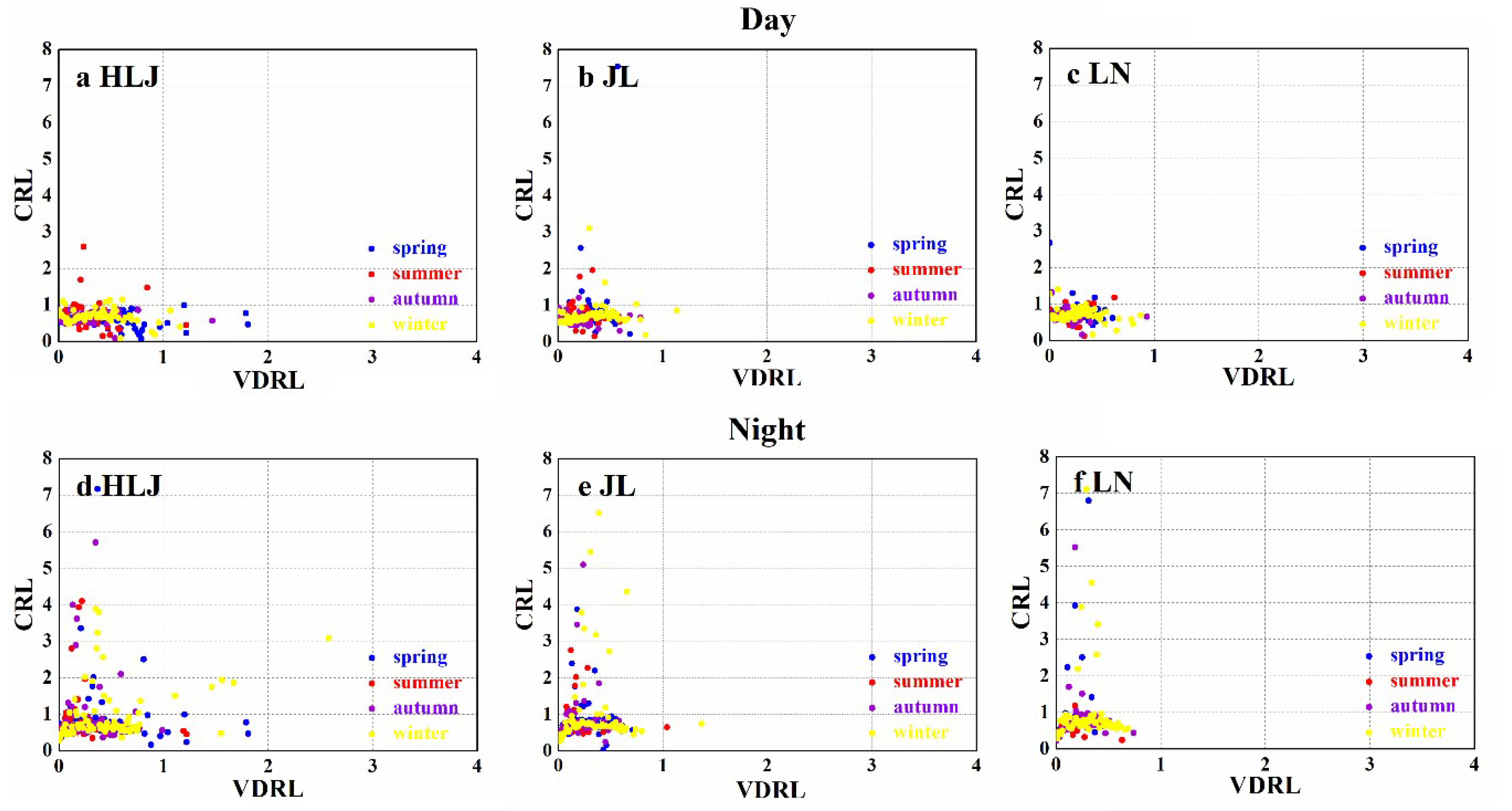
• The values of VDRL and CRL are higher in the daytime because of human activities.
• It is observed that AODL and TLL are weakly exponentially correlated; N and TAH are strongly linearly correlated, and N and PAODL are negatively correlated throughout the whole NEC.

Overall, these results provide a detailed and substantive scientific insight into the optical and physical properties of the aerosol layer over the Northeast of China. This knowledge would help frame a strategy for the management and treatment of air pollution over the NEC region.

References

1. Jansen, M. Intergovernmental Panel on Climate Change (IPCC). Encycl. Energy Nat. Resour. Environ. Econ. 2013, 2, 48–56. [Google Scholar]
2. Kaufman, Y.J.T.D.; Boucher, O. A satellite view of aerosols in the climate system. Nature 2002, 419, 215–223. [Google Scholar] [CrossRef] [PubMed]
3. Kulmala, M.; Kontkanen, J.; Junninen, H.; Lehtipalo, K.; Manninen, H.E.; Nieminen, T.; Petaja, T.; Sipila, M.; Schobesberger, S.; Rantala, P. Direct observations of atmospheric aerosol nucleation. Science 2013, 339, 943–946. [Google Scholar] [CrossRef] [PubMed]
4. Lelieveld, J.; Evans, J.S.; Fnais, M.; Giannadaki, D.; Pozzer, A. The contribution of outdoor air pollution sources to premature mortality on a global scale. Nature 2015, 525, 367–371. [Google Scholar] [CrossRef] [PubMed]
5. Rogge, W.F.; Hildemann, L.M.; Mazurek, M.A.; Cass, G.R.; Simoneit, B.R.T. Sources of fine organic aerosol. 5. Natural gas home appliances. Environ. Sci. Technol. 1993, 27, 2736–2744. [Google Scholar] [CrossRef]
6. Qiu, R.; Han, G.; Ma, X.; Xu, H.; Shi, T.; Zhang, M. A comparison of oco-2 sif, modis gpp, and gosif data from gross primary production (GPP) estimation and seasonal cycles in North America. Remote Sens. 2020, 12, 258. [Google Scholar] [CrossRef] [Green Version]
7. Edenhofer, O. Climate Change 2014: Mitigation of Climate Change: Working Group III Contribution to the Fifth Assessment Report of the Intergovernmental Panel on Climate Change; Cambridge University Press: Cambridge, UK, 2014. [Google Scholar]
8. Rosenfeld, D. Suppression of rain and snow by urban and industrial air pollution. Int. J. Food Microbiol. 2000, 287, 40–50. [Google Scholar] [CrossRef]
9. Twomey, S. The influence of pollution on the shortwave albedo of clouds. J. Atmos. Sci. 1977, 34, 1149–1154. [Google Scholar] [CrossRef] [Green Version]
10. Magistrale, V. Health Aspects of Air Pollution; Springer: Berlin/Heidelberg, Germany, 1992. [Google Scholar]
11. Qin, W.; Liu, Y.; Wang, L.; Lin, A.; Xia, X.; Che, H.; Bilal, M.; Zhang, M. Characteristic and driving factors of aerosol optical depth over mainland China during 1980–2017. Remote Sens. 2018, 10, 1064. [Google Scholar] [CrossRef] [Green Version]
12. Qin, Y.; Oduyemi, K. Atmospheric aerosol source identification and estimates of source contributions to air pollution in Dundee, UK. Atmos. Environ. 2003, 37, 1799–1809. [Google Scholar] [CrossRef]
13. Ramanathan, V.; Crutzen, P.J.; Kiehl, J.T. Aerosols, climate, and the hydrological cycle. Science 2005, 294, 2119–2126. [Google Scholar] [CrossRef] [PubMed] [Green Version]
14. Ramanathan, V.; Chung, C.; Kim, D.; Bettge, T.; Buja, L.; Kiehl, J.T.; Washington, W.M.; Fu, Q.; Sikka, D.R.; Wild, M. Atmospheric brown clouds: Impacts on south asian climate and hydrological cycle. Proc. Natl. Acad. Sci. USA 2005, 102, 5326–5333. [Google Scholar] [CrossRef] [PubMed] [Green Version]
15. Bilal, M.; Nichol, J.E. Evaluation of modis aerosol retrieval algorithms over the Beijing-Tianjin-Hebei region during low to very high pollution events. J. Geophys. Res. Atmos. 2015, 120, 7941–7957. [Google Scholar] [CrossRef] [Green Version]
16. Han, D.; Liu, W.; Zhang, Y.; Lu, Y.; Liu, J.; Yu, T. An Atmospheric Aerosol Lidar and Its Experiment in Beijing. 2007. Available online: https://spie.org/Publications/Proceedings/Paper/10.1117/12.747079?SSO=1 (accessed on 30 April 2020).
17. Parrish, D.D.; Tong, Z. Climate change. Clean air for megacities. Science 2009, 326, 674–675. [Google Scholar] [CrossRef] [PubMed]
18. Zhang, C.H.; Zhao, T.L.; Wang, F.; Xu, X.D.; Su, H.; Cheng, X.H.; Tan, C.H. Variations in Aerosol Optical Depth over Three Northeastern Provinces of China, in 2003–2014. Environ. Sci. China 2017. [Google Scholar] [CrossRef]
19. Chen, W.; Tong, D.Q.; Zhang, S.; Zhang, X.; Zhao, H. Local pm10 and pm2.5 emission inventories from agricultural tillage and harvest in northeastern China. J. Environ. Sci. 2017, 57, 15–23. [Google Scholar] [CrossRef]
20. Ho, K.F.; Zhang, R.J.; Lee, S.C.; Ho, S.S.H.; Liu, S.X.; Fung, K.; Cao, J.J.; Shen, Z.X.; Xu, H.M. Characteristics of carbonate carbon in pm2.5 in a typical semi-arid area of northeastern China. Atmos. Environ. 2011, 45, 1268–1274. [Google Scholar] [CrossRef]
21. Ho, C.H.; Choi, Y.S.; Hur, S.K. Long-term changes in summer weekend effect over northeastern China and the connection with regional warming. Geophys. Res. Lett. 2009, 36, 15. [Google Scholar] [CrossRef]
22. Dubovik, O.; Smirnov, A.; Holben, B.N.; King, M.D.; Kaufman, Y.J.; Eck, T.F.; Slutsker, I. Accuracy assessments of aerosol optical properties retrieved from aerosol robotic network (aeronet) sun and sky radiance measurements. J. Geophys. Res. Atmos. 2000, 105, 9791–9806. [Google Scholar] [CrossRef] [Green Version]
23. Smirnov, A.; Holben, B.N.; Eck, T.F.; Slutsker, I.; Chatenet, B.; Pinker, R.T. Diurnal variability of aerosol optical depth observed at aeronet aerosol robotic network sites. Geophys. Res. Lett. 2002, 29, 1–30. [Google Scholar] [CrossRef]
24. Omar, A.H.; Won, J.G.; Winker, D.M.; Yoon, S.C.; Dubovik, O.; McCormick, M.P. Development of global aerosol models using cluster analysis of aerosol robotic network aeronet measurements. J. Geophys. Res. Space Phys. 2005, 110, 10–14. [Google Scholar] [CrossRef]
25. Bilal, M.; Nichol, J.E.; Wang, L. New customized methods for improvement of the modis c6 dark target and deep blue merged aerosol product. Remote Sens. Environ. 2017, 197, 115–124. [Google Scholar] [CrossRef]
26. Kleidman, R.G.; O’Neill, N.T.; Remer, L.A.; Kaufman, Y.J.; Eck, T.F.; Tanré, D.; Dubovik, O.; Holben, B.N. Comparison of moderate resolution imaging spectroradiometer (modis) and aerosol robotic network (aeronet) remote-sensing retrievals of aerosol fine mode fraction over ocean. J. Geophys. Res. Atmos. 2005, 110, 22. [Google Scholar] [CrossRef]
27. Chu, D.A.; Kaufman, Y.J.; Ichoku, C.; Remer, L.A.; Tanré, D.; Holben, B.N. Validation of modis aerosol optical depth retrieval over land. Geophys. Res. Lett. 2002, 29, 8007. [Google Scholar] [CrossRef] [Green Version]
28. Wei, J.; Sun, L. Comparison and evaluation of different modis aerosol optical depth products over the Beijing-Tianjin-Hebei region in China. IEEE J. Sel. Top. Appl. Earth Obs. Remote Sens. 2017, 99, 1–10. [Google Scholar] [CrossRef]
29. Georgoulias, A.K.; Alexandri, G.; Kourtidis, K.A.; Lelieveld, J.; Zanis, P.; Amiridis, V. Differences between the modis collection 6 and 5.1 aerosol datasets over the greater mediterranean region. Atmos. Environ. 2016, 147, 310–319. [Google Scholar] [CrossRef]
30. Bilal, M.; Nichol, J.E. Evaluation of the ndvi-based pixel selection criteria of the modis c6 dark target and deep blue combined aerosol product. IEEE J. Sel. Top. Appl. Earth Obs. Remote Sens. 2017, 10, 3448–3453. [Google Scholar] [CrossRef]
31. Remer, L.A.; Tanré, D.; Kaufman, Y.J.; Ichoku, C.; Mattoo, S.; Levy, R.; Chu, D.A.; Holben, B.; Dubovik, O.; Smirnov, A. Validation of modis aerosol retrieval over ocean. Geophys. Res. Lett. 2002, 29, MOD3-1–MOD3-4. [Google Scholar] [CrossRef] [Green Version]
32. Winker, D.M.; Pelon, J. The Calipso Mission, Geoscience and Remote Sensing Symposium; IEEE International: Toulouse, France, 2003. [Google Scholar]
33. Winker, D.M.; Tackett, J.L.; Getzewich, B.J.; Liu, Z.; Vaughan, M.A.; Rogers, R.R. The global 3-d distribution of tropospheric aerosols as characterized by caliop. Atmos. Chem. Phys. 2013, 13, 3345–3361. [Google Scholar] [CrossRef] [Green Version]
34. Sayer, A.M.; Hsu, N.C.; Bettenhausen, C.; Jeong, M.J. Validation and uncertainty estimates for modis collection 6 “deep blue” aerosol data. J. Geophys. Res. Atmos. 2013, 118, 7864–7872. [Google Scholar] [CrossRef] [Green Version]
35. Winker, D.M.; Pelon, J.; Coakley, J.A., Jr.; Ackerman, S.A.; Charlson, R.J.; Colarco, P.R.; Flamant, P.; Hoff, R.M.; Kittaka, C. The calipso mission: A global 3d view of aerosols and clouds. Bull. Am. Meteorol. Soc. 2010, 91, 1211–1229. [Google Scholar] [CrossRef]
36. Winker, D.M.; Pelon, J.R.; Mccormick, M.P. The calipso mission: Spaceborne lidar for observation of aerosols and clouds. Bull. Am. Meteorol. Soc. 2010, 91, 1211–1229. [Google Scholar] [CrossRef]
37. Winker, D.M.; Vaughan, M.A.; Omar, A.; Hu, Y.; Powell, K.A.; Liu, Z.; Young, S.A. Overview of the calipso mission and caliop data processing algorithms. J. Atmos. Ocean. Technol. 2009, 26, 2310–2323. [Google Scholar] [CrossRef]
38. Winker, D.M.; Hunt, W.H.; McGill, M.J. Initial performance assessment of caliop. Geophys. Res. Lett. 2007, 34, 228–262. [Google Scholar] [CrossRef] [Green Version]
39. Zhang, M.; Liu, J.; Bilal, M.; Zhang, C.; Zhao, F.; Xie, X.; Khedher, K.M. Optical and physical characteristics of the lowest aerosol layers over the yellow river basin. Atmosphere 2019, 10, 638. [Google Scholar] [CrossRef] [Green Version]
40. Bi, J.; Huang, J.; Fu, Q.; Wang, X.; Shi, J.; Zhang, W.; Huang, Z.; Zhang, B. Toward characterization of the aerosol optical properties over loess plateau of northwestern China. J. Quant. Spectrosc. Radiat. Transf. 2011, 112, 346–360. [Google Scholar] [CrossRef]
41. Xia, X.; Zong, X.; Cong, Z.; Chen, H.; Kang, S.; Wang, P. Baseline continental aerosol over the central Tibetan plateau and a case study of aerosol transport from south Asia. Atmos. Environ. 2011, 45, 7370–7378. [Google Scholar] [CrossRef]
42. Zhang, M.; Wang, L.; Bilal, M.; Gong, W.; Zhang, Z.; Guo, G. The characteristics of the aerosol optical depth within the lowest aerosol layer over the Tibetan Plateau from 2007 to 2014. Remote Sens. 2018, 10, 696. [Google Scholar] [CrossRef] [Green Version]
43. Wu, Z.J.; Ma, N.; Größ, J.; Kecorius, S.; Lu, K.D.; Shang, D.J.; Wang, Y.; Wu, Y.S.; Zeng, L.M.; Hu, M. Thermodynamic properties of nanoparticles during new particle formation events in the atmosphere of North China plain. Atmos. Res. 2017, 188, 55–63. [Google Scholar] [CrossRef]
44. Zhang, S.L.; Ma, N.; Kecorius, S.; Wang, P.C.; Hu, M.; Wang, Z.B.; Groess, J.; Wu, Z.J.; Wiedensohler, A. Mixing state of atmospheric particles over the North China plain. Atmos. Environ. 2016, 125, 152–164. [Google Scholar] [CrossRef] [Green Version]
45. Xu, C.; Ma, Y.M.; You, C.; Zhu, Z.K. The regional distribution characteristics of aerosol optical depth over the Tibetan plateau. Atmos. Chem. Phys. 2015, 15, 12065–12078. [Google Scholar] [CrossRef] [Green Version]
46. Liu, Y.; Huang, J.; Shi, G.; Takamura, T.; Zhang, B. Aerosol optical properties determined from sky-radiometer over loess plateau of northwest China. Atmos. Chem. Phys. Discuss. 2011, 11, 23883–23910. [Google Scholar] [CrossRef] [Green Version]
47. Tian, P.; Cao, X.; Zhang, L.; Wang, H.; Shi, J.; Huang, Z.; Zhou, T.; Liu, H. Observation and simulation study of atmospheric aerosol nonsphericity over the loess plateau in northwest China. Atmos. Environ. 2015, 117, 212–219. [Google Scholar] [CrossRef]
48. Liu, Z.; Zheng, Y.F.; Liu, J.J.; Xie, M.Q. Research on the distribution of the northern region of China aerosol based on a-trian satellite. China Environ. Sci. 2015, 35, 2891–2898. [Google Scholar]
49. Ding, T.; Chen, L.; Cui, D.; Center, N.C. Decadal variations of summer precipitation in northeast China and the associated circulation. Plateau Meteorol. 2015, 34, 220–229. [Google Scholar]
50. Mcgrath-Spangler, E.L.; Denning, A.S. Global seasonal variations of midday planetary boundary layer depth from calipso space-borne lidar. J. Geophys. Res. Atmos. 2013, 118, 1226–1233. [Google Scholar] [CrossRef]
51. Zhang, M.; Ma, Y.; Gong, W.; Zhu, Z. Aerosol optical properties of a haze episode in wuhan based on ground-based and satellite observations. Atmosphere 2014, 5, 699–719. [Google Scholar] [CrossRef] [Green Version]
52. Zhang, M.; Liu, J.; Bilal, M.; Zhang, C.; Nazeer, M.; Atique, L.; Han, G.; Gong, W. Aerosol optical properties and contribution to differentiate haze and haze-free weather in Wuhan city. Atmophere 2020, 11, 322. [Google Scholar] [CrossRef] [Green Version]
53. Wang, X.; Huang, J.; Zhang, R.; Chen, B.; Bi, J. Surface measurements of aerosol properties over northwest China during arm China 2008 deployment. J. Geophys. Res. 2010, 115. [Google Scholar] [CrossRef] [Green Version]
54. Huang, J.Z.W.; Zuo, J.; Bi, J.; Shi, J.; Wang, X.; Chang, Z.; Huang, Z.; Yang, S.; Zhang, S. An overview of the semi-arid climate and environment research observatory over the loess plateau. Adv. Atmos. Sci. 2008, 25, 906. [Google Scholar] [CrossRef]
55. Dey, S.; Girolamo, L.D. A climatology of aerosol optical and microphysical properties over the Indian subcontinent from 9 years (2000–2008) of multiangle imaging spectroradiometer (MISR) data. J. Geophys. Res. Atmos. 2010, 115. [Google Scholar] [CrossRef] [Green Version]
56. Fu, R.H.Y.; Wright, J.S.; Jiang, J.H.; Dickinson, R.E.; Chen, M.; Filipiak, M.; Read, W.G.; Waters, J.W.; Wu, D.L. Short circuit of water vapor and polluted air to the global stratosphere by convective transport over the Tibetan plateau. Proc. Natl. Acad. Sci. USA 2006, 103, 5664–5669. [Google Scholar] [CrossRef] [Green Version]
Figure 1. The geographical location of Northeastern China (NEC). The color bar represents the altitude (elevation).
Atmosphere 11 00501 g001
Figure 2. Inter-annual variations in the optical and physical properties of aerosol layers over NEC (Heilongjiang province (HLJ), Jilin province (JL), and Liaoning province (LN)) in the daytime from 2007 to 2014. (a) The AOD of all the aerosol layers (AODA), (b) the base altitude of the lowest aerosol layer (BAL), (c) the top altitude of the highest aerosol layer (TAH), (d) the number of aerosol feature layers (N), (e) the AOD of the lowest aerosol layer (AODL), (f) the thickness of the lowest aerosol layer (TLL), (g) the AOD proportion of the lowest aerosol layer (PAODL), (h) the volume depolarization ratio of the lowest aerosol layer (VDRL), and (i) the color ratio of the lowest aerosol layer (CRL).
Atmosphere 11 00501 g002
Figure 3. Inter-annual variations in the optical and physical properties of aerosol layers over NEC (HLJ, JL, and LN) in the nighttime from 2007 to 2014. (a) AODA, (b) BAL, (c) TAH, (d) N, (e) AODL, (f) TLL, (g) PAODL, (h) VDRL, and (i) CRL.
Atmosphere 11 00501 g003
Figure 4. Inter-annual spatial distributions of AODA, BAL, TAH, N, AODL, TLL, PAODL, VDRL, and CRL over NEC (HLJ, JL, and LN) in the daytime, from 2007 to 2014.
Atmosphere 11 00501 g004
Figure 5. Inter-annual spatial distributions of AODA, BAL, TAH, N, AODL, TLL, PAODL, VDRL, and CRL over NEC (HLJ, JL, and LN) in the nighttime, from 2007 to 2014.
Atmosphere 11 00501 g005
Figure 6. Seasonal variations in the optical and physical properties of aerosol layers over NEC (HLJ, JL, and LN) in the daytime, from 2007 to 2014. (a) AODA, (b) BAL, (c) TAH, (d) N, (e) AODL, (f) TLL, (g) PAODL, (h) VDRL, and (i) CRL.
Atmosphere 11 00501 g006
Figure 7. Seasonal variations in the optical and physical properties of aerosol layers over NEC (HLJ, JL, and LN) in the nighttime, from 2007 to 2014. (a) AODA, (b) BAL, (c) TAH, (d) N, (e) AODL, (f) TLL, (g) PAODL, (h) VDRL, and (i) CRL.
Atmosphere 11 00501 g007
Figure 8. Seasonal spatial distributions of AODA, BAL, TAH, N, AODL, TLL, PAODL, VDRL, and CRL over NEC (HLJ, JL, and LN) in the daytime.
Atmosphere 11 00501 g008
Figure 9. Seasonal spatial distributions of AODA, BAL, TAH, N, AODL, TLL, PAODL, VDRL, and CRL over NEC (HLJ, JL, and LN) in the nighttime.
Atmosphere 11 00501 g009
Figure 10. The correlation between AODL and TLL over NEC. Where, (a,d) represent HLJ, (b,e) represent JL, and (c,f) represent LN.
Atmosphere 11 00501 g010
Figure 11. The correlation between TAH and N over NEC. Where, (a,d) represent HLJ, (b,e) represent JL, and (c,f) represent LN.
Atmosphere 11 00501 g011
Figure 12. The correlation between PAODL and N over NEC. Where, (a,d) represent HLJ, (b,e) represent JL, and (c,f) represent LN.
Atmosphere 11 00501 g012
Figure 13. The correlation between CRL and VDRL over NEC. Where, (a,d) represent HLJ, (b,e) represent JL, and (c,f) represent LN.
Atmosphere 11 00501 g013