Stochastic Resonance Observed in Aerosol Optical Depth Time Series

Abstract

We analyzed the aerosol optical depth time series retrieved from daily satellite Moderate-Resolution Imaging Spectroradiometer measurements. The investigated geographic area includes Italy and the Mediterranean Sea. By performing second- and fourth-order statistics analyses, the dynamics can be decomposed into two sources, the main of which is the annual cycle. The residence time distribution is made of local maxima over an exponential behavior. The two successive peaks are located at about 200 and 600 days. This allows us to hypothesize a stochastic resonance phenomenon in the dynamics of aerosol optical depth. The characteristic periodicity of the resonance is on the annual timescale, and the asymmetric double-well potential is provided by two different regimes for the values of the aerosol optical depth in winter and summer time. This means that a simple, although stochastic, differential equation can represent the time evolution of the optical depth, at least concerning its component related to the annual cycle.

1. Introduction

Atmospheric aerosol particles influence the Earth’s radiation balance directly, by the scattering and the absorption of the incoming solar radiation and indirectly by changing the albedo, the clouds recovering, acting as condensation nuclei, and air quality, this playing a relevant role in the greenhouse effect [1,2,3]. The total tropospheric aerosol is mainly (for about 40%) affected by desert dust [4].

The understanding of the aerosol particles’ impact on the regional and global climate change is one of the most relevant problems in climate modeling. To account for the spatial and temporal variability of the aerosols, remote sensing from satellites delivers information about global aerosol distribution.

A well-defined physical quantity measuring these effects is aerosol optical depth (AOD). It is determined by subtracting the contributions of the total column ozone absorption, water vapor absorption and Rayleigh scattering from the total atmospheric optical depth as provided by the known Lambert–Beer law.

In the literature, many studies investigated AOD on a long-term scale, focusing attention on the related spectral properties, and the correlations with air temperature and precipitation (see, e.g., [5,6,7,8,9,10]). Indeed, the spectral properties of aerosol optical properties influence the Ångström parameters and the aerosol radiative properties (aerosol phase function, single scattering albedo) [11].

In this work, AOD time evolution is analyzed considering a geographic area including Italy and the Mediterranean Sea. The investigated area represents a significant case study for aerosols, because the high solar radiation intensity and the cloud-free conditions strongly affect the climate especially in summertime. Moreover, proximity to regions such as the Western Sahara influences the Mediterranean Sea producing large aerosol optical depths [4,12]. Regarding the Mediterranean area, dust mainly originates from the Sahara Desert and is transported to Europe (see, e.g., [13] and references therein). This region includes a variety of geographical areas (urban, desert, marine) with different types of aerosols.

The main goal of this work is to derive information on the aerosol in order to develop a model able to reproduce its dynamics at least on the selected spatial scale. In other words, we study and characterize the AOD in the framework of dynamical system theory in order to describe the associated complex dynamics by exploiting differential equations. In a seminal work, for the same geographic area, a stochastic resonance mechanism was recognized to play a fundamental role in the dynamics of the Aerosol Index (AI) [14]. The annual peak in the AI power spectrum was, indeed, interpreted in terms of an activated resonance. It would be interesting if a stochastic mechanism is still governing the dynamics of AOD, which is an indicator of air transparency and thus a more quantitative parameter than AI.

Stochastic resonance (RS) is a general mechanism observed in a large variety of physical systems such as lasers, semiconductor devices, chemical reactions, neurophysiological and biological systems, virus dynamics (see, e.g., [15,16,17,18]). RS describes phenomena where a weak periodic signal can be amplified and optimized by the presence of noise. Of course, in the case of natural systems, the environmental noise, which affects all the dynamics, can change in intensity over time, and its contribution must be extracted from the experimental data. The interaction between the environmental noise and the nonlinearity gives rise to a rich variety of experimental phenomenology and dynamic behaviors from climate to biological systems [19,20,21,22,23]. In addition, fluctuations may play a relevant role in stabilizing the dynamics of metastable systems (see [24,25,26]).

2. Experiments

This work analyzes the time series of AOD retrieved from daily satellite Moderate-Resolution Imaging Spectroradiometer (MODIS) measurements. For an updated analysis on the MODIS system and the set of associated data, see Wei et al. 2019 [27].

The dataset consists of 200 time series of AOD at 550 nm, measured daily for the period from February 2000 to March 2006, for each point of a geographical grid whose spatial extension comprises the Mediterranean area, going from 6° W–9° E and 34° W–43° N, with a resolution of about 10² km × 10² km.

Gaps in the regional coverage of MODIS retrievals, mostly due to the cloud coverage, to the difficulties with highly reflective arid and snow-covered land [5] are filled with a random extraction of missing data from a log-normal distribution parameterized by the statistical estimates of raw data. Indeed, in the atmosphere, the size distributions of aerosols, clouds and parameters of turbulent processes follow a log-normal distribution law [28].

For each time series, we calculate the mean and the standard deviation of the logarithm of the AOD values and use them as parameters of the corresponding log-normal distribution.

Missing data represent about 24% of the whole dataset, with a density which gets larger and larger going towards the northeast. The log-normal filling algorithm provides a quite effective procedure to supply lost data. For each time series j (j = 1,..., 200), whose number of elements is denoted with n, we calculate the geometric mean µ_j and the geometric standard deviation σ_j of the AOD values ${\tau }_i^j$ for i= 1,…n, and use them as parameters of the corresponding log-normal distribution:

$$P\left(\log \left({\tau }_i\right)\right)=\frac{\exp \left(\frac{{(\log \left({\tau }_i^j\right)-\log \left({\mu }_j\right))}^2}{2{\log }^2\left({\sigma }_j\right)}\right)}{\sqrt{2\pi }\log \left({\sigma }_j\right)}$$

(1)

Hence, each gap in the j-th time series is filled with a value extracted from the distribution (Equation (1)).

3. Results

3.1. Linear and Nonlinear Analysis

We characterize the AOD series in terms of dynamical systems by adopting both linear and nonlinear analyses. Indeed, we retrieve the spectral properties information on the underlying sources and their degrees of freedom.

Figure 1a displays the behavior of a typical AOD signal, and Figure 1b shows the relative amplitude distribution. Notice that the black stars superimposed on the histogram represent the distribution of the AOD values calculated following Equation (1), showing quite a good accordance between simulated and raw data.

Even at a glance, the AOD signal shows a periodicity in its time evolution. To better investigate this characterization, spectral analysis is performed.

Figure 2 shows the normalized power spectrum in logarithmic scale stacked over the 200 series. It represents the overall dynamics much better than an individual spectrum relative to just one series, and, of course, relative to just one story of our process.

The spectrum evidences the existence of a complex system, in which the highest peak corresponds to an annual cycle and additionally its harmonics are also evident. At very high frequency, i.e., on the scale of a week, a peak at about 2–3 days emerges.

Regarding the latter, although it emerges also in the mean value, the peak is too close to the Nyquist frequency to comment on, leaving its further investigation to data with a higher sampling.

The annual peak, on the other hand, marks the influence of seasonal phenomena on the aerosol concentration in the atmosphere, and hence on the corresponding AOD (see, e.g., [29]). In the following, we focus on this annual cycle, which is strongly affected by the Saharan dust [4,12,13] in our investigated area.

In order to identify the dynamical system generating the experimental AOD, we apply a decomposition method in time domain, that is, the Independent Component Analysis (ICA) to the whole dataset. It is an entropy-based technique, which can find underlying components (sources) from multivariate statistical data based on their statistical independence. The latter is evaluated by using fourth-order statistical properties. Its goal is to find a linear representation of non-Gaussian data so that the components are statistically independent, or as independent as possible. ICA relies upon the Central Limit Theorem, which implies that the sum of two independent random variables has a distribution closer to Gaussian than any of the two original random variables [30,31,32]. ICA has been already successfully applied to a variety of experimental signals, such as in the field of volcano seismology and oceanography [33,34,35,36,37,38,39,40].

Figure 3 shows the results relative to the application of ICA to AOD series, displaying the waveforms and the relative PSDs of the extracted components (ICs). By avoiding some redundancies in ICs, it is possible to identify two components with a well-separated spectral content. Indeed, IC1 has a dominant peak of about 1 year, which appears on a sustained background noise, as shown in Figure 3a. Indeed, the annual contribution is not extracted as an independent periodic signal linearly superposed to the noise [30], suggesting that the annual periodic part in these signals is intrinsically tied to the fluctuations. Instead, IC2 is characterized by a period of about 2–3 days as reported in Figure 3b. Finally, IC3 represents the residual (Figure 3c). Summarizing, the 2–3 days periodicity is extracted as an independent source in time domain, whereas the annual periodicity is expected to be generated by genuine stochastic dynamics [15].

Considering the ICA results, in the following, we concentrate on the dynamic characterization of the annual cycle.

To achieve that goal, an estimate of the reconstructed phase space dimension is derived. We apply the false nearest neighbors method (FNN) [41] to each time series of the dataset. The method is used for the embedding dimension estimate. This technique is based on the projection of the points of the dynamics onto spaces of increasing dimensions. The points appear as nearest neighbors of some others until the dimension becomes that of the embedding space. When the fraction of these false nearest neighbors with respect to the total number of points is zero, the process is complete [41]. Note that the value thus obtained represents the lower limit for the embedding dimension necessary to evaluate attractor dimension on which the asymptotic dynamics evolves.

The application of the technique provides a singular and fascinating result: For all the time series, there is no convergence of the algorithm up to a dimension equal to 10.

This means that the results of the phase space analysis are incompatible with both a deterministic and a chaotic evolution of the system, but in accordance with possible stochastic dynamics.

3.2. AOD Residence Time Distribution and Modeling

Now, we are interested in characterizing the larger temporal variations of AOD, i.e., understanding the dynamical origin of the annual peak. Hence, we focus our analysis and the following numerical simulations on this portion of the spectrum. The raw signals are low-pass filtered selecting the corner frequency at 10⁻⁶ Hz. Due to the difference in depth and typology of the aerosol layers between winter and summer, we can distinguish two different regimes for the values of the AOD. It is reasonable to hypothesize that there are two metastable states which characterize the seasonal amount of AOD.

The distribution of the time intervals between two consecutive metastable states, known as Residence Time Distribution (RTD), gives information about the stochastic behavior of the AOD dynamics, and it quantifies the degree of synchronization at each switching [41,42,43,44,45,46]. The residence times are estimated introducing a set of coupled thresholds τ_u and τ_d, fixed according to the average values of AOD during winter and summer, respectively, and taking the time necessary to cross them (residence times). To simplify the comparison between the observed data and those obtained by the numerical simulations of the dynamic model, we make each signal a null-average time series, shifting accordingly the values of the thresholds. Thus, for each couple of thresholds, we apply an appropriate residence time counting algorithm to each time series. Subsequently, due to the relative shortness of the signals considered, the time intervals have been aggregated to get more significant statistics. Specifically, for τ_u= 0.2 and τ_d= −0.15, the resulting RTD of our analysis is shown in Figure 4.

The RTD histogram shows exponentially decreasing peaks. The first significant peak is centered between 190 and 210 days, while the second one is located around 600 days. We remark that the RTD exhibits the typical exponential form in a pure noisy two-state system, whereas, in presence of a periodic forcing, with period T_Ω, and in regime of SR, one observes a series of exponentially decreasing peaks, the first of which is (nearly) centered at the stochastic transition time T_s = T_Ω/2, which represents the timescale matching condition for stochastic resonance [16,47].

The nonmonotonic behavior of the residence time as a function of noise has been crucial in investigating many experimental phenomena (see, e.g., [24,25,26] and references therein).

The RTD of Figure 4 is in accordance with the hypothesis of a SR mechanism for the dynamics of the AOD: In particular, the first peak of the RTD (about 190 days) is centered approximately at half of T_Ω (381 days looking at the low frequency peak in the spectrum of Figure 2), providing the aforementioned timescale matching condition for the stochastic resonance.

3.3. Stochastic Resonance Modeling

We assume that the transitions between the two states are driven by a combined action of a periodic forcing and a noise term which considers the atmospheric complexity. Thus, the dynamics of the system can be described by an SR model with a double-well potential modulated by a periodic component and added to a stochastic fluctuation term [15,16,17,18,19].

That hypothesis is in accordance with the seminal paper of De Martino et al. (2002) [15], where an SR mechanism was recognized to play a fundamental role in the interpretation of the annual peak in the power spectrum of the Aerosol Index.

The typical signal to noise ratio curve of the stochastic resonance for the analyzed data is reported in Figure 5. As one can see, with respect to the level of noise, in this geographic area, AOD is close to the maximum. This means that though the resonance is not fully developed, most of the energy is taken from the noise. The previous results assure us that AOD experiences a phenomenon of SR. In addition, the difference between the absolute values of the thresholds suggests an asymmetrical double-well potential for the SR model, yielding relevant constraints for the parameters of the model. Very recently, the noise-stabilizing effects were also observed in quantum systems with asymmetric bi-stable potentials [14,15,25].

Specifically, if the potential has the form:

$$V\left(x\right)=\frac{x^4}{4}-\frac{\mathrm{a} x^3}{3}-\frac{\mathrm{b} x^2}{2}$$

(2)

with a and b positive parameters, and S_u and S_d denoting the values of the thresholds, with |S_u|>|S_d|, self-consistent arguments lead to the following constraints:

a≥|S_u|>|S_d|    b≥|S_u||S_d|

(3)

Thus, the equation of our stochastic resonance model for the dynamics of the AOD is:

dx = −V’(x)dt + Acos(ωt)dt + νdξ;

(4)

where x is representative of AOD, the periodic forcing (A,ω) takes into account the annual cycle affected by the Saharan dust, ν is the noise level and dξ is a Wiener process. The asymmetric double-well potential represents the different height of the aerosol layers in winter and summer, which is a consequence of the radiative balance of incoming and outcoming radiation at the top of the atmosphere (following the Budyko–Sellers model). The model requires the estimates of two parameters: the amplitude A and the level of noise ν, having fixed the frequency to the annual cycle, and the parameters of the asymmetric double-well potential (a = 0.02 and b = 0.07). Specifically, for each couple of (A,ν) values, we performed 200 numerical simulations of the dynamics of the AOD according to the SR model. The best couple of (A, ν) was selected minimizing the distance between the mean values, at each time, of the time simulated and raw data. The correlation between the two averaged signals is maximized (greater than 0.7). With this criterion, we obtained an estimate of A = 10⁻³ and ν = 0.02, respectively.

The superposition of the simulated signal and experimental average signal is shown in Figure 6.

4. Discussion and Conclusions

We performed a detailed analysis of AOD in the Mediterranean area, including Italy, characterizing the experimental series in terms of second- and fourth-order statistics. Moreover, we derived a mathematical model for describing the observed data.

Summarizing, the results presented in this work are:

(1)

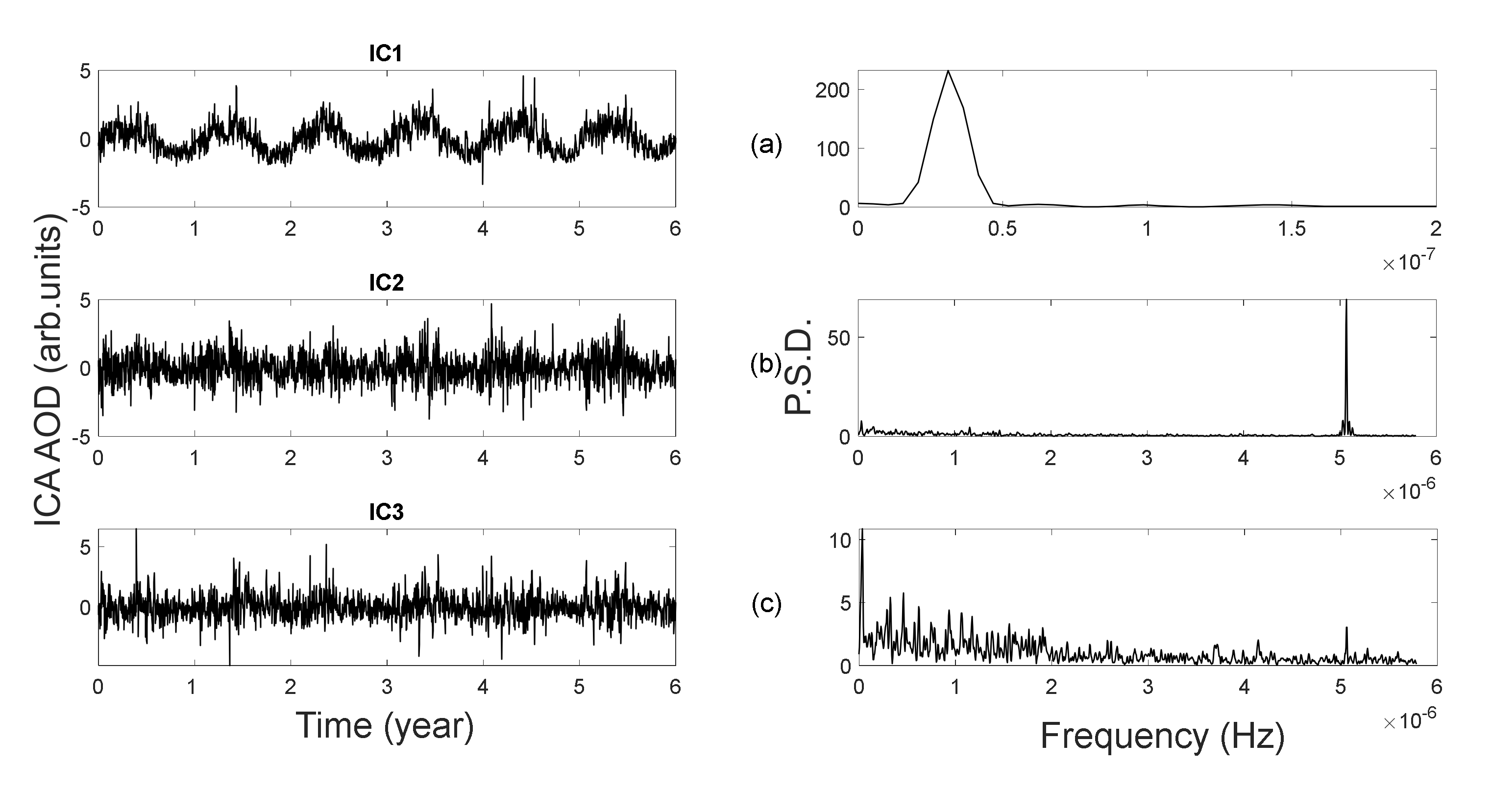
AOD is made of a wide band spectrum in which a peak characterized by an annual periodicity emerges retaining most of the information. A non-negligible contribution at very high frequency of the order of a few days is also present.

(2)

ICA basically decomposes AOD into two main and independent signals (time components), IC1 (peaked at about 1 year) and IC2 (peaked at about 2–3 days). The first extracted signal component IC1 is the most energetic.

(3)

The residence time distribution is made of local maxima over an exponential behavior. The two successive peaks are located at about 200 and 600 days.

(4)

FNN indicates that there is no convergence of the algorithm up to a dimension equal to 10, showing no high dimensional deterministic system is driving the dynamics.

All previous results suggest that the annual cycle, well extracted in ICA, is intrinsically tied to the fluctuations and, thus, described by a stochastic process. The residence time distribution provides the stochastic transition time between two stable states. Based on all these results, we can ascribe the annual cycle (IC1) to a phenomenon of stochastic resonance. The comparison between a standard SR model and our data indicates an asymmetric double-well potential in Equation (4), a periodic contribution on the annual scale (periodicity of IC1) and noise.

Though over a smaller investigated area, De Martino et al. (2002) [15] demonstrated the same SR mechanism for the AI. We demonstrate that a stochastic behavior and a consequent SR mechanism also arise in a larger geographic area when analyzing the physical AOD parameter.

The noise that influences, on a local scale, the standard optical properties through a resonant behavior is presumably produced for the major part over urban areas; nevertheless, it influences a very large area. The investigated parameter AOD has been conjectured and, in some cases, shown to influence local meteorological behavior. Our result introduces an equation that governs the dynamics and allows a quantitative estimate of the parameters relevant to AOD on a local scale.

References

1. Lolli, S.; Khor, W.Y.; Matjafri, M.Z.; Lim, H.S. Monsoon Season Quantitative Assessment of Biomass Burning Clear-Sky Aerosol Radiative Effect at Surface by Ground-Based Lidar Observations in Pulau Pinang, Malaysia in 2014. Remote Sens. 2019, 11, 2660. [Google Scholar] [CrossRef] [Green Version]
2. Alfaro-Contreras, R.; Zhang, J.; Reid, J.S.; Christopher, S. A study of 15-year aerosol optical thickness and direct shortwave aerosol radiative effect trends using MODIS, MISR, CALIOP and CERES. Atmos. Chem. Phys. 2017, 17, 13849–13868. [Google Scholar] [CrossRef] [Green Version]
3. Pérez, C.; Sicard, M.; Jorba, O.; Comerón, A.; Baldasano, J.M. Summertime re-circulations of air pollutants over the north-eastern Iberian coast observed from systematic EARLINET lidar measurements in Barcelona. Atmos. Environ. 2004, 38, 3983–4000. [Google Scholar] [CrossRef]
4. Papayannis, V.; Amiridis, L.; Mona, G.; Tsaknakis, D.; Balis, D.; Bösenberg, J.; Chaikovski, A.; de Tomasi, F.; Grigorov, I.; Mattis, I.; et al. Systematic lidar observations of Saharan dust over Europe in the frame of EARLINET (2000–2002). J. Geophys. Res. Atmos. Am. Geophys. Union 2008, 113. [Google Scholar] [CrossRef] [Green Version]
5. Yu, H.; Dickinson, R.E.; Chin, M.; Kaufman, Y.J.; Holben, B.N.; Geogdzhayev, I.V.; Mishchenko, M.I. Annual cycle of global distributions of aerosol optical depth from integration of MODIS retrievals and GOCART model simulations. J. Geophys. Res. 2003, 108, 4128. [Google Scholar] [CrossRef]
6. O’Neill, N.T.; Pancrati, O.; Baibakov, K.; Eloranta, E.; Batchelor, R.L.; Freemantle, J.; McArthur, L.J.B.; Strong, K.; Lindenmaier, R. Occurrence of weak, sub-micron, tropospheric aerosol events at high Arctic latitudes. Geophys. Res. Lett. 2008, 35, L14814. [Google Scholar] [CrossRef] [Green Version]
7. Loeb, N.G.; Schuster, G.L. An observational study of the relationship between cloud, aerosol and meteorology in broken low-level cloud conditions. J. Geophys. Res. 2008, 113, D14214. [Google Scholar] [CrossRef] [Green Version]
8. Ranjan, R.R.; Joshi, H.P.; Iyer, K.N. Spectral Variation of Total Column Aerosol Optical Depth over Rajkot: A Tropical Semi-arid Indian Station. Aerosol Air Qual. Res. 2007, 7, 33–45. [Google Scholar] [CrossRef] [Green Version]
9. Reid, J.S.; Lagrosas, N.D.; Jonsson, H.H.; Reid, E.A.; Atwood, S.A.; Boyd, T.J.; Ghate, V.P.; Xian, P.; Posselt, D.J.; Simpas, J.B.; et al. Aerosol meteorology of Maritime Continent for the 2012 7SEAS southwest monsoon intensive study—Part 2: Philippine receptor observations of fine-scale aerosol behavior. Atmos. Chem. Phys. 2016, 16, 14057–14078. [Google Scholar] [CrossRef] [Green Version]
10. Campbell, J.R.; Ge, C.; Wang, J.; Welton, E.J.; Bucholtz, A.; Hyer, E.J.; Reid, E.A.; Chew, B.N.; Liew, S.-C.; Salinas, S.; et al. Applying Advanced Ground-Based Remote Sensing in the Southeast Asian Maritime Continent to Characterize Regional Proficiencies in Smoke Transport Modeling. J. Appl. Meteorol. Climatol. 2016, 55. [Google Scholar] [CrossRef]
11. Eck, T.F.; Holben, B.N.; Reid, J.S.; Dubovic, O.; Smirnov, A.; O’Neil, N.T.; Slutsker, I.; Kinne, S. Wavelength dependence of the optical depth of biomass burning, urban, and desert dust aerosols. J. Geophys. Res. 1999, 104, 31333–31349. [Google Scholar] [CrossRef]
12. Papadimas, C.D.; Hatzianastassiou, N.; Mihalopoulos, N.; Querol, X.; Vardavas, I. Spatial and temporal variability in aerosol properties over the Mediterranean basin based on 6-year (2000–2006) MODIS data. J. Geophys. Res. 2008, 113, D11205. [Google Scholar] [CrossRef]
13. Di Iorio, T.; di Sarra, A.; Sferlazzo, D.M.; Cacciani, M.; Meloni, D.; Monteleone, F.; Fuà, D.; Fiocco, G. Seasonal evolution of the tropospheric aerosol vertical profile in the central Mediterranean and role of desert dust. J. Geophys. Res. 2009, 114, D02201. [Google Scholar] [CrossRef] [Green Version]
14. Cuomo, V.; de Martino, S.; Falanga, M.; Mona, L. Influence of local dust source and stochastic fluctuations on Saharan aerosol index dynamics. Int. J. Mod. Phys. B 2009, 23, 5383–5390. [Google Scholar] [CrossRef]
15. De Martino, S.; Falanga, M.; Mona, L. Stochastic resonance mechanism in Aerosol Index dynamics. Phys. Rev. Lett. 2002, 89, 128501. [Google Scholar] [CrossRef] [PubMed] [Green Version]
16. Gammaitoni, L.; Hanggi, P.; Jung, P.; Marchesoni, F. Stochastic Resonance. Rev. Mod. Phys. 1998, 70, 223–287. [Google Scholar] [CrossRef]
17. Lanzara, E.; Mantegna, R.N.; Spagnolo, B.; Zangara, R. Experimental study of a nonlinear system in the presence of noise: The stochastic resonance. Am. J. Phys. 1997, 65, 341–349. [Google Scholar] [CrossRef]
18. Mantegna, R.N.; Spagnolo, B.; Trapanese, M. Linear and nonlinear experimental regimes of stochastic resonance. Phys. Rev. E 2001, 63, 011101. [Google Scholar] [CrossRef] [Green Version]
19. Spezia, S.; Curcio, L.; Fiasconaro, A.; Pizzolato, N.; Valenti, D.; Spagnolo, B.; Bue, P.L.; Peri, E.; Colazza, S. Evidence of stochastic resonance in the mating behavior of Nezara viridula. Eur. Phys. J. B 2008, 65, 453–458. [Google Scholar] [CrossRef]
20. Ditlevsen, P.D.; Svensmark, H.; Johnsen, S. Contrasting atmospheric and climate dynamics of the last-glacial and Holocene periods. Nature 1996, 379, 810–812. [Google Scholar] [CrossRef]
21. Ditlevsen, P.D. Observation of alpha-stable noise induced millennial climate changes from an ice-core record. Geophys. Res. Lett. 1999, 26, 1441–1444. [Google Scholar] [CrossRef] [Green Version]
22. Caruso, A.; Gargano, M.E.; Valenti, D.; Fiasconaro, A.; Spagnolo, B. Cyclic Fluctuations, Climatic Changes and Role of Noise in Planktonic Foraminifera in the Mediterranean Sea. Fluct. Noise Lett. 2005, 5, L349–L355. [Google Scholar] [CrossRef] [Green Version]
23. Valenti, D.; Tranchina, L.; Brai, M.; Caruso, A.; Cosentino, C.; Spagnolo, B. Environmental metal pollution considered as noise: Effects on the spatial distribution of benthic foraminifera in two coastal marine areas of Sicily (Southern Italy). Ecol. Model. 2008, 213, 449–462. [Google Scholar] [CrossRef] [Green Version]
24. Spagnolo, B.; Valenti, D.; Guarcello, C.; Carollo, A.; Adorno, D.P.; Spezia, S.; Pizzolato, N.; di Paola, B. Noise-induced effects in nonlinear relaxation of condensed matter systems. Chaos Solitons Fractals 2015, 81, 412–424. [Google Scholar] [CrossRef]
25. Valenti, D.; Magazzù, L.; Caldara, P.; Spagnolo, B. Stabilization of quantum metastable states by dissipation. Phys. Rev. B 2015, 91, 235412. [Google Scholar] [CrossRef] [Green Version]
26. Spagnolo, B.; Guarcello, C.; Magazzù, L.; Carollo, A.; Persano Adorno, D.; Valenti, D. Nonlinear Relaxation Phenomena in Metastable Condensed Matter Systems. Entropy 2017, 19, 20. [Google Scholar] [CrossRef] [Green Version]
27. Wei, J.; Li, Z.; Peng, Y.; Sun, L. MODIS Collection 6.1 aerosol optical depth products over land and ocean: Validation and comparison. Atmos. Environ. 2019, 201, 428–440. [Google Scholar] [CrossRef]
28. Limpert, E.; Werner, A.S.; Abbt, M. Log-normal Distributions across the Sciences: Keys and Clues: On the charms of statistics, and how mechanical models resembling gambling machines offer a link to a handy way to characterize log-normal distributions, which can provide deeper insight into variability and probability—Normal or log-normal: That is the question. BioScience 2001, 51, 341–352. [Google Scholar]
29. Li, F.; Ramanathan, V. Winter to summer monsoon variation of aerosol optical depth over the tropical Indian Ocean. J. Geophys. Res. 2002, 107. [Google Scholar] [CrossRef]
30. De Lauro, E.; De Martino, S.; Falanga, M.; Ciaramella, A.; Tagliaferri, R. Complexity of time series associated to dynamical systems inferred from independent component analysis. Phys. Rev. E 2005, 72, 046712. [Google Scholar] [CrossRef]
31. Hyvarinen, A.; Karhunen, J.; Oja, E. Independent Component Analysis; Wiley and Sons: New York, NY, USA, 2001. [Google Scholar]
32. Ciaramella, A.; De Lauro, E.; Martino, S.; Falanga, M.; Tagliaferri, R. ICA based identification of dynamical systems generating synthetic and real world time series. Soft Comput. 2008, 10, 587–606. [Google Scholar] [CrossRef]
33. De Martino, S.; Falanga, M.; Palo, M.; Montalto, M.; Patanè, D. Statistical analysis of the seismicity during the Strombolian crisis of 2007, Italy: Evidence of a precursor in tidal range. J. Geophys. Res. 2010, 116, B09312. [Google Scholar] [CrossRef]
34. Capuano, P.; De Lauro, E.; De Martino, S.; Falanga, M.; Petrosino, S. Convolutive independent component analysis for processing massive datasets: A case study at Campi Flegrei (Italy). Nat. Hazards 2017, 86, 417–429. [Google Scholar] [CrossRef]
35. Capuano, P.; De Lauro, E.; De Martino, S.; Falanga, M. Detailed investigation of Long-Period activity at Campi Flegrei by Convolutive Independent Component Analysis. Phys. Earth Planet. Int. 2016, 253, 48. [Google Scholar] [CrossRef]
36. De Lauro, E.; De Martino, S.; Falanga, M.; Palo, M. Statistical analysis of Stromboli VLP tremor in the band [0.1–0.5] Hz: Some consequences for vibrating structures. Nonlinear Process. Geophys. 2006, 13, 393–400. [Google Scholar] [CrossRef] [Green Version]
37. De Lauro, E.; Petrosino, S.; Ricco, C.; Aquino, I.; Falanga, M. Medium and long period ground oscillatory pattern inferred by borehole tiltmetric data: New perspectives for the Campi Flegrei caldera crustal dynamics. Earth Planet. Sci. Lett. 2018, 504, 21–29. [Google Scholar] [CrossRef]
38. De Lauro, E.; De Martino, S.; Falanga, M.; Riente, M.A. Far-field synoptic wind effects extraction from sea-level oscillations: The Venice lagoon case study. Estuar. Coast. Shelf Sci. 2018, 210, 18–25. [Google Scholar] [CrossRef]
39. De Lauro, E.; De Martino, S.; Falanga, M.; Petrosino, S. Fast wavefield decomposition of volcano-tectonic earthquakes into polarized P and S waves by Independent Component Analysis. Tectonophysics 2016, 290, 355–361. [Google Scholar] [CrossRef]
40. Cusano, P.; Petrosino, S.; De Lauro, E.; Falanga, M. The whisper of the hydrothermal seismic noise at Ischia Island. J. Volcanol. Geotherm. Res. 2019, 389, 106693-1–106693-10. [Google Scholar] [CrossRef]
41. Abarbanel, H.D.I.; Brown, R.; Sidorowich, J.J.; Tsimring, L.S. The analysis of observed chaotic data in physical systems. Rev. Mod. Phys. 1993, 65, 1331–1392. [Google Scholar] [CrossRef] [Green Version]
42. Gammaitoni, L.; Marchesoni, F.; Menichella-Saetta, E.; Santucci, S. Resonant crossing processes controlled by colored noise. Phys. Rev. Lett. 1993, 71, 3625. [Google Scholar] [CrossRef]
43. Zhou, T.; Moss, F.; Jung, P. Escape-time distributions of a periodically modulated bistable system with noise. Phys. Rev. A 1990, 42, 3161. [Google Scholar] [CrossRef]
44. Löfstedt, R.; Coppersmith, S.N. Stochastic resonance: Nonperturbative calculation of power spectra and residence-time distributions. Phys. Rev. E 1994, 49, 4821. [Google Scholar] [CrossRef]
45. Choi, M.H.; Fox, R.F.; Jung, P. Quantifying stochastic resonance in bistable systems: Response vs residence-time distribution functions. Phys. Rev. E 1998, 57, 6335–6344. [Google Scholar] [CrossRef]
46. Giacomelli, G.; Marin, F.; Rabbiosi, I. Stochastic and bona fide resonance: An experimental investigation. Phys. Rev. Lett. 1999, 82, 675–678. [Google Scholar] [CrossRef]
47. Wellens, T.; Shatokhin, V.; Buchleitner, A. Stochastic resonance. Rep. Prog. Phys. 2004, 67, 45–105. [Google Scholar] [CrossRef]
Figure 1. (a) An example of the gap-filled data and (b) the relative distribution, which the log-normal distribution is superposed to (black stars). A strong periodicity is visible in the waveform.
Atmosphere 11 00502 g001
Figure 2. Normalized power spectrum (PSD) in semilogarithmic scale stacked over the 200 series of aerosol optical depth (AOD): A dominant peak is associated with the annual cycle, but also higher harmonics are evident up to a week timescale.
Atmosphere 11 00502 g002
Figure 3. Independent Component Analysis (ICA) extracted components and relative PSDs: (a) The annual peak is always embedded in a background noise (IC1), linking noise to the deterministic part, whereas (b) a 2–3 day period (IC2) is completely separated; (c) residual is represented by IC3.
Atmosphere 11 00502 g003
Figure 4. Residence time distribution (RTD): Two main peaks centered between 190 and 210 days, and around 600 days can be observed. The typical exponential decreasing peaks support a stochastic resonance phenomenon in the dynamics of AOD [16]. This represents an example of estimate of the residence times (the lapsed times) between the two selected amplitude-crossing thresholds τu = 0.2 and τd = −0.15.
Atmosphere 11 00502 g004
Figure 5. Signal to noise ratio curve: The maximum corresponds to a fully developed resonance. The red star corresponds to our level of resonance. From comparison with the experimental series, the level of noise is 0.02, whereas for a full resonance, the model requires a level of noise equal to about 0.03.
Atmosphere 11 00502 g005
Figure 6. Comparison between simulated (red line) and experimental data (black line). Performing numerical simulations, the best fit with data under the constraints of Equation (3) leads to A= 10−3 and ν ≈ 0.03 at resonance.
Atmosphere 11 00502 g006