How Cool Are Allotment Gardens? A Case Study of Nocturnal Air Temperature Differences in Berlin, Germany

 ,
,
Abstract
1. Introduction
- How does the mean nocturnal of AGs differ from densely built-up areas (URB), urban parks and rural areas (RUR) in the study area?
- How and to what extent, do mean differences between URB and AGs correlate with micro-scale land surface characteristics of AGs?
2. Materials and Methods
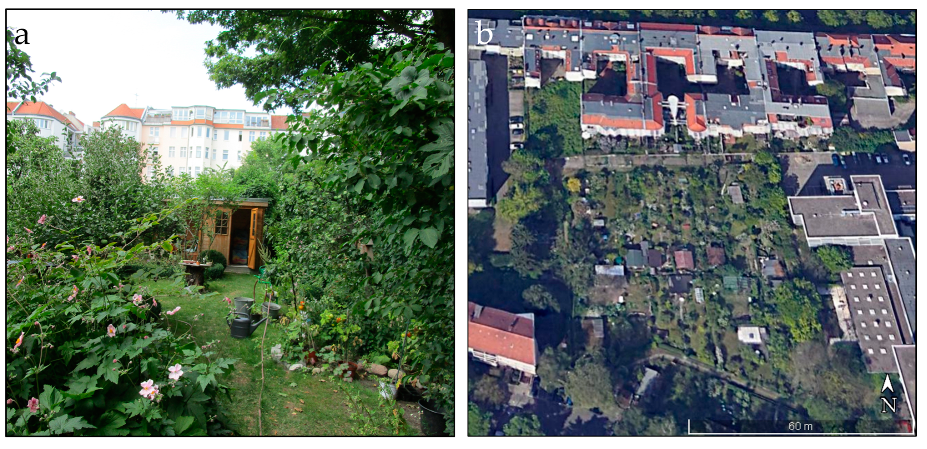
2.1. Study Area
2.2. Selection of Measurement Sites and Land Surface Characteristics of AGs and Surroundings
2.3. Measurement Campaign
2.4. Data Preparation
2.5. Data Processing
3. Results
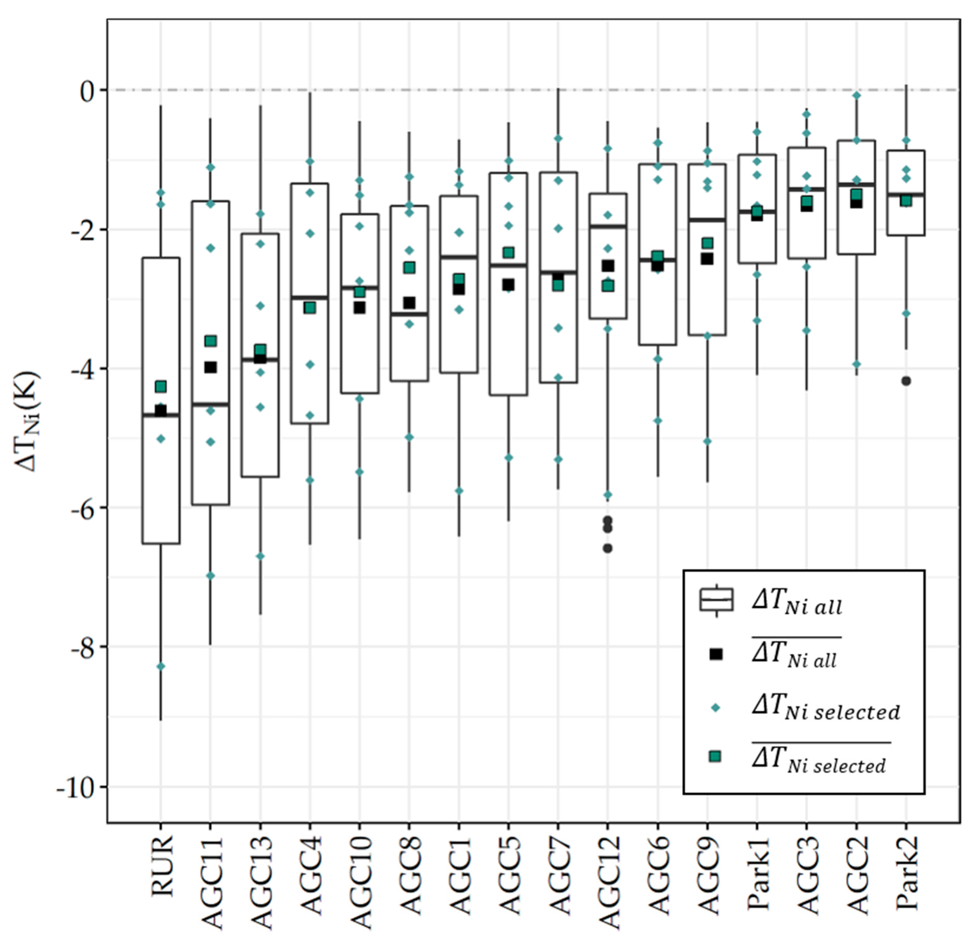
3.1. Nocturnal Air Temperature Differences
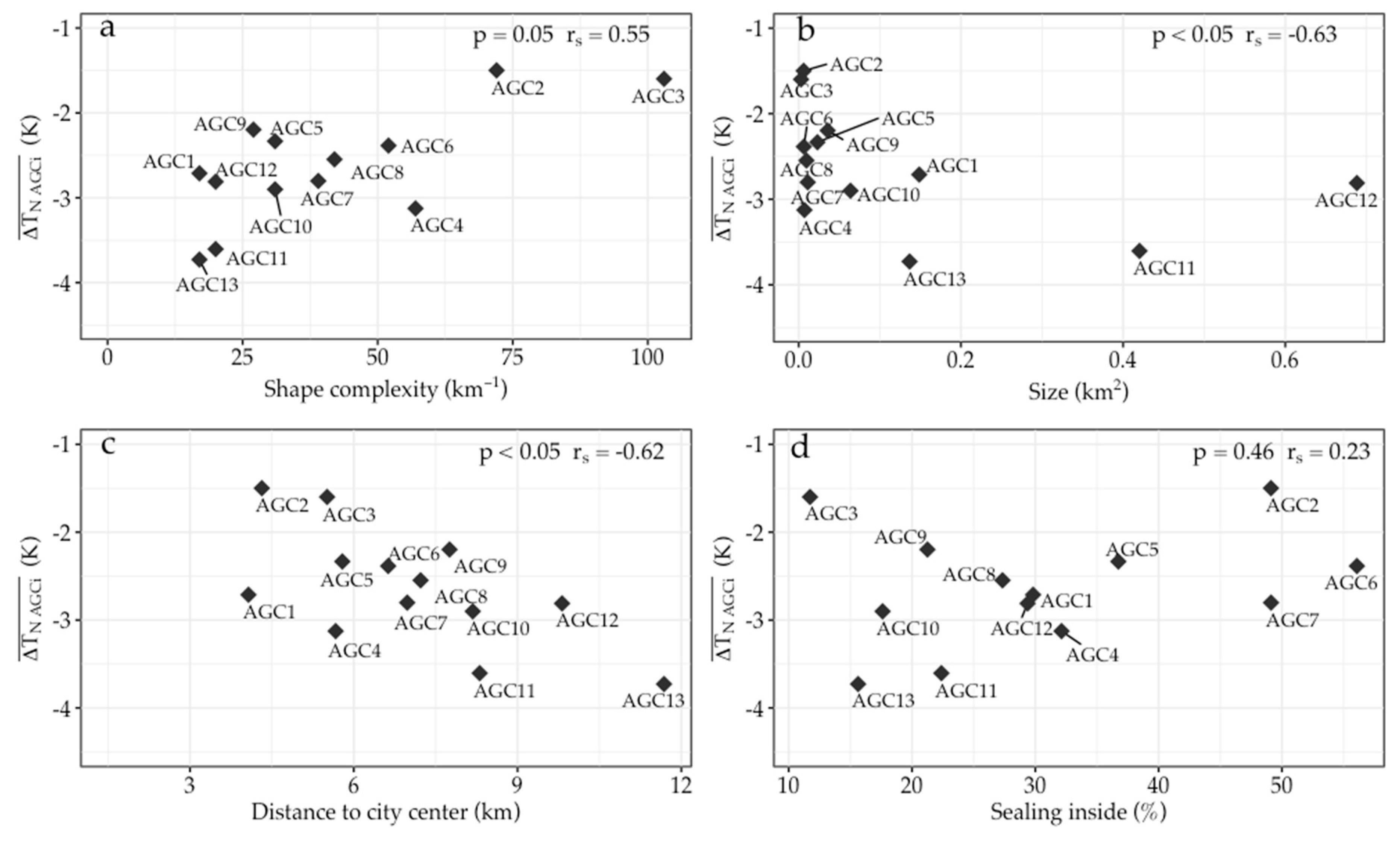
3.2. Correlation between Land Surface Characteristics and Nocturnal Air Temperature Differences
4. Discussion
4.1. Nocturnal Air Temperature Differences between AGCs and URB
4.2. Nocturnal Air Temperature Differences between AGCs, Urban Parks and RUR
4.3. Land Surface Characteristics
5. Conclusions
Author Contributions
Funding
Acknowledgments
Conflicts of Interest
Appendix A

Appendix B

| ID | RUR | Park1 | Park2 | URB | |||
|---|---|---|---|---|---|---|---|
| Station | Kaniswall, KANI | Dahlemer Feld, DAHF | Tiergarten | Tempelhofer Feld | Alexanderplatz, ALEX | Bamberger Straße, BAMB | Dessauer Straße, DESS |
| Operator | DWD | TUB | TUB | DWD | DWD | TUB | TUB |
| Latitude/Longitude | 52.4040 N/13.7309 E | 52.4777 N/13.2252 E | 52.5145 N/13.3636 E | 52.4675 N/13.4021 E | 52.5198 N/13.4054 E | 52.4964 N/13.3375 E | 52.5045 N/13.3783 E |
| Site elevation (m) | 33.0 | 51.0 | 34.0 | 48.0 | 36.0 | 36.0 | 33.5 |
| Size (km2) | – | – | 2.1 | 3.0 | – | – | – |
| Perimeter (km) | – | – | 22.63 | 7.34 | – | – | – |
| Shape complexity (km−1) | – | – | 0.09 | 0.41 | – | – | – |
| Distance to city center (km) | 25.0 | 13.1 | 3.0 | 4.9 | 0.0 | 5.5 | 2.6 |
| FSI inside/outside (-) | –/0.00 | –/0.74 | 0.06/0.36 | 0.12/0.36 | –/0.74 | –/2.37 | –/1.69 |
| Sealing in-/outside (%) | –/1.50 | –/0.0 | 6.18/42.46 | 24.66/35.33 | –/73.43 | –/70.07 | –/61.48 |
| LCZ | B | A | D | 2 | |||
| SVF (-) | 0.9 | 0.46 | 0.16 | 0.96 | 0.54 | 0.24 | 0.42 |
| (selected) (°C) | 15.5 | 18.0 | 18.1 | 19.7 | |||
| (all) (°C) | 12.8 | 15.9 | 15.7 | 17.4 | |||
| (selected) (K) | −4.3 | −1.7 | −1.6 | – | |||
| (all) (K) | −4.6 | −1.8 | −1.6 | – | |||
| max/min(selected) (K) | −1.5/−8.3 | −0.6/−3.3 | −0.7/−3.2 | – | |||
| max/min(all) (K) | −0.2/−9.1 | −0.5/−4.1 | 0.1/−4.2 | – | |||
| ID | AGC1 | AGC2 | AGC3 | AGC4 | |||||||||||||||
|---|---|---|---|---|---|---|---|---|---|---|---|---|---|---|---|---|---|---|---|
| Logger ID | 1a | 1b | 1c | 2a | 2b | 3a | 3b | 4a | 4b | 4c | |||||||||
| Latitude/Longitude | 52.56519 N/13.404214 E | 52.557609 N/13.404278 E | 52.556801 N/13.404211 E | 52.544499 N/13.357116 E | 52.544136 N/13.357093 E | 52.526632 N/13.260129 E | 52.523865 N/13.325949 E | 52.499702 N/13.483952 E | 52.499840 N/13.483896 E | 52.499641 N/13.483865 E | |||||||||
| Shape |  |  |  |  | |||||||||||||||
| Scale | 1:35,000 | 1:8500 | 1:10,000 | 1:8500 | |||||||||||||||
| Site elevation (m) | 46.5 | 36.5 | 33.5 | 34.5 | |||||||||||||||
| Size (km2) | 0.15 | 0.006 | 0.003 | 0.007 | |||||||||||||||
| Perimeter (km) | 2.55 | 0.44 | 0.3 | 0.4 | |||||||||||||||
| Shape complexity (km−1) | 17.1 | 71.8 | 103.2 | 56.7 | |||||||||||||||
| Distance to city center (km) | 4.1 | 4.3 | 5.5 | 5.7 | |||||||||||||||
| FSI in-/outside (-) | 0.01/0.87 | 0.78/1.80 | 0.00/1.89 | 0.00/0.38 | |||||||||||||||
| Sealing in-/outside (%) | 29.82/49.61 | 49.11/61.84 | 11.73/71.13 | 32.12/46.88 | |||||||||||||||
| SVF (-) | 0.93 | 0.8 | 0.71 | 0.91 | 0.77 | 0.79 | 0.74 | 0.93 | 0.92 | 0.86 | |||||||||
| (selected) (°C) | 17.0 | 18.2 | 18.1 | 16.6 | |||||||||||||||
| (all) (°C) | 14.5 | 15.8 | 15.7 | 14.3 | |||||||||||||||
| (selected) (K) | −1.7 | −1.5 | −1.6 | −3.1 | |||||||||||||||
| (all) (K) | −2.9 | −1.6 | −1.7 | −3.1 | |||||||||||||||
| max/min(selected) (K) | −1.2/−5.8 | −0.1/−3.9 | −0.3/−3.5 | −1.0/−5.6 | |||||||||||||||
| max/min(all) (K) | −0.7/−6.4 | −0.1/−4.1 | −0.3/−4.3 | 0.0/−6.5 | |||||||||||||||
| ID | AGC5 | AGC6 | AGC7 | AGC8 | |||||||||||||||
| Logger ID | 5a | 5b | 6a | 6b | 6c | 7a | 7b | 8a | 8b | ||||||||||
| Latitude/Longitude | 52.476465 N/13.453303 E | 52.476300 N/13.454340 E | 52.522476 N/13.272697 E | 52.483948 N/13.329340 E | 52.484454 N/13.328883 E | 52.506701 N/13.506705 E | 52.506472 N/13.507516 E | 52.565796 N/13.331121 E | 52.566356 N/13.332066 E | ||||||||||
| Shape |  |  |  |  | |||||||||||||||
| Scale | 1:10,000 | 1:10,000 | 1:10,000 | 1:10,000 | |||||||||||||||
| Site elevation (m) | 33.5 | 36.5 | 38 | 57.75 | |||||||||||||||
| Size (km2) | 0.02 | 0.006 | 0.011 | 0.01 | |||||||||||||||
| Perimeter (km) | 0.71 | 0.33 | 0.44 | 0.4 | |||||||||||||||
| Shape complexity (km−1) | 30.8 | 51.5 | 39.4 | 42.3 | |||||||||||||||
| Distance to city center (km) | 5.8 | 6.6 | 7.0 | 7.2 | |||||||||||||||
| FSI in-/outside (-) | 0.46/0.96 | 2.00/1.93 | 0.56/0.92 | 0.27/0.60 | |||||||||||||||
| Sealing in-/outside (%) | 36.73/57.56 | 56.08/60.55 | 49.12/50.8 | 27.34/42.23 | |||||||||||||||
| SVF (-) | 0.76 | 0.9 | 0.51 | 0.81 | 0.8 | 0.85 | 0.59 | 0.82 | 0.89 | ||||||||||
| (selected) (°C) | 17.4 | 17.4 | 16.9 | 16.2 | |||||||||||||||
| (all) (°C) | 14.6 | 14.9 | 14.7 | 14.4 | |||||||||||||||
| (selected) (K) | −2.3 | −2.4 | −2.8 | −2.5 | |||||||||||||||
| (all) (K) | −2.8 | −2.5 | −2.7 | −3.1 | |||||||||||||||
| max/min(selected) (K) | −1.0/−5.3 | −0.8/−4.7 | −0.7/−5.3 | −1.2/−5.0 | |||||||||||||||
| max/min(all) (K) | −0.5/−6.2 | −0.5/−5.6 | 0.0/−5.7 | −0.6/−5.8 | |||||||||||||||
| ID | AGC9 | AGC10 | AGC11 | ||||||||||||||||
| Logger ID | 9a | 9b | 9c | 10a | 10b | 10c | 11a | 11b | 11c | ||||||||||
| Latitude/Longitude | 52.487628 N/13.307651 E | 52.487071 N/13.306620 E | 52.486057 N/13.305941 E | 52.474764 N/13.311752 E | 52.473863 N/13.312507 E | 52.474095 N/13.313315 E | 52.456609 N/13.474660 E | 52,456151 N/13.474205 E | 52,456078 N/13.464090 E | ||||||||||
| Shape |  |  |  | ||||||||||||||||
| Scale | 1:20,000 | 1:20,000 | 1:40,000 | ||||||||||||||||
| Site elevation (m) | 44.5 | 41.2 | 33.83 | ||||||||||||||||
| Size (km2) | 0.04 | 0.06 | 0.42 | ||||||||||||||||
| Perimeter (km) | 0.96 | 1.98 | 8.33 | ||||||||||||||||
| Shape complexity (km−1) | 26.9 | 31.0 | 19.8 | ||||||||||||||||
| Distance to city center (km) | 7.8 | 8.2 | 8.3 | ||||||||||||||||
| FSI in-/outside (-) | 0.00/0.96 | 0.26/1.16 | 0.02/0.31 | ||||||||||||||||
| Sealing in-/outside (%) | 21.25/56.76 | 17.61/50.67 | 22.38/32.73 | ||||||||||||||||
| SVF (-) | 0.86 | 0.75 | 0.94 | 0.92 | 0.92 | 0.72 | 0.92 | 0.96 | 0.82 | ||||||||||
| (selected) (°C) | 17.5 | 16.8 | 16.1 | ||||||||||||||||
| (all) (°C) | 15.0 | 14.3 | 13.4 | ||||||||||||||||
| (selected) (K) | −2.2 | −2.9 | −3.6 | ||||||||||||||||
| (all) (K) | −2.4 | −3.1 | −4.0 | ||||||||||||||||
| max/min(selected) (K) | −0.9/−5.0 | −1.3/- 5.5 | −1.1/−7.0 | ||||||||||||||||
| max/min(all) (K) | −0.5/−5.6 | −0.4/−6.5 | −0.4/−8.0 | ||||||||||||||||
| ID | AGC12 | AGC13 | |||||||||||||||||
| Logger ID | 12a | 12b | 12c | 12d | 12e | 13a | 13b | ||||||||||||
| Latitude/Longitude | 52,523609 N/13.325962 E | 52.526377 N/13.267863 E | 52.522101 N/13.271471 E | 52.483956 N/13.328949 E | 52.522335 N/13.269297 E | 52.529149 N/13.578040 E | 52.530704 N/13.580143 E | ||||||||||||
| Shape |  |  | |||||||||||||||||
| Scale | 1:40,000 | 1:40,000 | |||||||||||||||||
| Site elevation (m) | 52.2 | 50 | |||||||||||||||||
| Size (km2) | 0.69 | 0.14 | |||||||||||||||||
| Perimeter (km) | 13.91 | 2.27 | |||||||||||||||||
| Shape complexity (km−1) | 20.2 | 16.6 | |||||||||||||||||
| Distance to city center (km) | 9.8 | 11.7 | |||||||||||||||||
| FSI in-/outside (-) | 0.03/0.44 | 0.00/0.21 | |||||||||||||||||
| Sealing in-/outside (%) | 29.37/37.19 | 15.63/19.45 | |||||||||||||||||
| SVF (-) | 0.93 | 0.91 | 0.9 | 0.79 | 0.85 | 0.95 | 0.72 | ||||||||||||
| (selected) (°C) | 16.9 | 16.0 | |||||||||||||||||
| (all) (°C) | 14.9 | 13.6 | |||||||||||||||||
| (selected) (K) | −2.8 | −3.7 | |||||||||||||||||
| (all) (K) | −2.5 | −3.8 | |||||||||||||||||
| max/min(selected) (K) | −0.8/−5.8 | −1.8/−6.7 | |||||||||||||||||
| max/min(all) (K) | −0.4/−6.6 | −0.2/−7.5 | |||||||||||||||||
Appendix C
| ID | AGCx | AGCy | AGC12 | |
|---|---|---|---|---|
| Logger ID | Xa | Xb | Ya | 12f |
| Shape |  |  |  | |
| Scale | 1:400,000 | 1:100,000 | 1:40,000 | |
| Latitude/Longitude | 52.478976 N/13.467163 E | 52.479141 N/13.466929 E | 52.522476 N/13.272697 E | 52.523577 N/13.269642 E |
| Reason for the exclusion of the data | Missing data: 81% | Missing data: 49% | Missing data: 21% | |
| Exclusion of Xa led to exclusion of AGCx, because the minimum number of two measurement stations per AGC was not provided. | ||||
References
- Gill, S.E.; Handley, J.F.; Ennos, A.R.; Pauleit, S. Adapting Cities for Climate Change: The Role of the Green Infrastructure. Built Environ. 2007, 33, 115–133. [Google Scholar] [CrossRef]
- Oke, T.R. The energetic basis of the urban heat island. Q. J. R. Meteorol. Soc. 1982, 108, 1–24. [Google Scholar] [CrossRef]
- Arnfield, A.J. Two decades of urban climate research: A review of turbulence, exchanges of energy and water, and the urban heat island. Int. J. Clim. 2003, 23, 1–26. [Google Scholar] [CrossRef]
- Fenner, D.; Meier, F.; Bechtel, B.; Otto, M.; Scherer, D. Intra and inter ‘local climate zone’ variability of air temperature as observed by crowdsourced citizen weather stations in Berlin, Germany. Meteorol. Z. 2017, 26, 525–547. [Google Scholar] [CrossRef]
- Oke, T.R. Street design and urban canopy layer climate. Energy Build. 1988, 11, 103–113. [Google Scholar] [CrossRef]
- Stewart, I.D.; Oke, T.R. Local Climate Zones for Urban Temperature Studies. Bull. Am. Meteorol. Soc. 2012, 93, 1879–1900. [Google Scholar] [CrossRef]
- Alexander, P.; Mills, G. Local Climate Classification and Dublin’s Urban Heat Island. Atmosphere 2014, 5, 755–774. [Google Scholar] [CrossRef]
- Mills, G. Luke Howard and The Climate of London. Weather 2008, 63, 153–157. [Google Scholar] [CrossRef]
- Dugord, P.-A.; Lauf, S.; Schuster, C.; Kleinschmit, B. Land use patterns, temperature distribution, and potential heat stress risk—The case study Berlin, Germany. Comput. Environ. Urban 2014, 48, 86–98. [Google Scholar] [CrossRef]
- Lauf, S.; Haase, D.; Kleinschmit, B. Linkages between ecosystem services provisioning, urban growth and shrinkage―A modeling approach assessing ecosystem service trade-offs. Ecol. Indic. 2014, 42, 73–94. [Google Scholar] [CrossRef]
- Doick, K.J.; Peace, A.; Hutchings, T.R. The role of one large greenspace in mitigating London’s nocturnal urban heat island. Sci. Total Environ. 2014, 493, 662–671. [Google Scholar] [CrossRef] [PubMed]
- Emmanuel, R.; Loconsole, A. Green infrastructure as an adaptation approach to tackling urban overheating in the Glasgow Clyde Valley Region, UK. Landsc. Urban Plan. 2015, 138, 71–86. [Google Scholar] [CrossRef]
- Chang, C.-R.; Li, M.-H.; Chang, S.-D. A preliminary study on the local cool-island intensity of Taipei city parks. Landsc. Urban Plan. 2007, 80, 386–395. [Google Scholar] [CrossRef]
- Spronken-Smith, R.A.; Oke, T.R. The thermal regime of urban parks in two cities with different summer climates. Int. J. Remote Sens. 1998, 19, 2085–2104. [Google Scholar] [CrossRef]
- Zardo, L.; Geneletti, D.; Pérez-Soba, M.; van Eupen, M. Estimating the cooling capacity of green infrastructures to support urban planning. Ecosyst. Serv. 2017, 26, 225–235. [Google Scholar] [CrossRef]
- Bowler, D.E.; Buyung-Ali, L.; Knight, T.M.; Pullin, A.S. Urban greening to cool towns and cities: A systematic review of the empirical evidence. Landsc. Urban Plan. 2010, 97, 147–155. [Google Scholar] [CrossRef]
- Larondelle, N.; Haase, D. Urban ecosystem services assessment along a rural–urban gradient: A cross-analysis of European cities. Ecol. Indic. 2013, 29, 179–190. [Google Scholar] [CrossRef]
- Höppe, P. Improving indoor thermal comfort by changing outdoor conditions. Energy Build. 1991, 16, 743–747. [Google Scholar] [CrossRef]
- Spronken-Smith, R.A.; Oke, T.R. Scale Modelling of Nocturnal Cooling in Urban Parks. Bound. Layer Meteorol. 1999, 93, 287–312. [Google Scholar] [CrossRef]
- Ren, Z.; He, X.; Zheng, H.; Zhang, D.; Yu, X.; Shen, G.; Guo, R. Estimation of the Relationship between Urban Park Characteristics and Park Cool Island Intensity by Remote Sensing Data and Field Measurement. Forests 2013, 4, 868–886. [Google Scholar] [CrossRef]
- Cao, X.; Onishi, A.; Chen, J.; Imura, H. Quantifying the cool island intensity of urban parks using ASTER and IKONOS data. Landsc. Urban Plan. 2010, 96, 224–231. [Google Scholar] [CrossRef]
- Feyisa, G.L.; Dons, K.; Meilby, H. Efficiency of parks in mitigating urban heat island effect: An example from Addis Ababa. Landsc. Urban Plan. 2014, 123, 87–95. [Google Scholar] [CrossRef]
- Hagishima, A.; Narita, K.-I.; Tanimoto, J. Field experiment on transpiration from isolated urban plants. Hydrol. Process. 2007, 21, 1217–1222. [Google Scholar] [CrossRef]
- Meier, F.; Scherer, D. Spatial and temporal variability of urban tree canopy temperature during summer 2010 in Berlin, Germany. Theor. Appl. Clim. 2012, 110, 373–384. [Google Scholar] [CrossRef]
- Upmanis, H.; Eliasson, I.; Lindqvist, S. The influence of green areas on nocturnal temperatures in a high latitude city (Göteborg, Sweden). Int. J. Clim. 1998, 18, 681–700. [Google Scholar] [CrossRef]
- Lin, B.B.; Egerer, M.H.; Liere, H.; Jha, S.; Bichier, P.; Philpott, S.M. Local- and landscape-scale land cover affects microclimate and water use in urban gardens. Sci. Total Environ. 2018, 610–611, 570–575. [Google Scholar] [CrossRef]
- Egerer, M.H.; Lin, B.B.; Threlfall, C.G.; Kendal, D. Temperature variability influences urban garden plant richness and gardener water use behavior, but not planting decisions. Sci. Total Environ. 2019, 646, 111–120. [Google Scholar] [CrossRef]
- Zölch, T.; Maderspacher, J.; Wamsler, C.; Pauleit, S. Using green infrastructure for urban climate-proofing: An evaluation of heat mitigation measures at the micro-scale. Urban For. Urban Green. 2016, 20, 305–316. [Google Scholar] [CrossRef]
- Koc, C.B.; Osmond, P.; Peters, A. Towards a comprehensive green infrastructure typology: A systematic review of approaches, methods and typologies. Urban Ecosyst. 2017, 20, 15–35. [Google Scholar] [CrossRef]
- Bell, S.; Fox-Kämper, R.; Keshavarz, N.; Benson, M.; Caputo, S.; Noori, S.; Voigt, A. (Eds.) Urban Allotment Gardens in Europe; Routledge: London, UK; New York, NY, USA, 2018; ISBN 978-1-138-92109-2. [Google Scholar]
- Cabral, I.; Keim, J.; Engelmann, R.; Kraemer, R.; Siebert, J.; Bonn, A. Ecosystem services of allotment and community gardens: A Leipzig, Germany case study. Urban For. Urban Green. 2017, 23, 44–53. [Google Scholar] [CrossRef]
- Cabral, I.; Costa, S.; Weiland, U.; Bonn, A. Urban Gardens as Multifunctional Nature-Based Solutions for Societal Goals in a Changing Climate. In Nature-Based Solutions to Climate Change Adaptation in Urban Areas; Kabisch, N., Korn, H., Stadler, J., Bonn, A., Eds.; Springer International Publishing: Cham, Switzerland, 2017; pp. 237–253. ISBN 978-3-319-53750-4. [Google Scholar]
- Senatsverwaltung für Umwelt, Verkehr und Klimaschutz. Daten und Fakten zu Kleingärten/Land Berlin. Available online: https://www.berlin.de/senuvk/umwelt/stadtgruen/kleingaerten/de/daten_fakten/index.shtml (accessed on 31 May 2018).
- Senatsverwaltung für Stadtentwicklung und Umwelt. Das bunte Grün. Kleingärten in Berlin. 2012. Available online: https://www.berlin.de/senuvk/umwelt/stadtgruen/kleingaerten/downloads/Kleingartenbroschuere.pdf (accessed on 31 May 2018).
- Armstrong, D. A survey of community gardens in upstate New York: Implications for health promotion and community development. Health Place 2000, 6, 319–327. [Google Scholar] [CrossRef]
- Edmondson, J.L.; Stott, I.; Davies, Z.G.; Gaston, K.J.; Leake, J.R. Soil surface temperatures reveal moderation of the urban heat island effect by trees and shrubs. Sci. Rep. 2016, 6, 33708. [Google Scholar] [CrossRef]
- Borysiak, J.; Mizgajski, A.; Speak, A. Floral biodiversity of allotment gardens and its contribution to urban green infrastructure. Urban Ecosyst. 2017, 20, 323–335. [Google Scholar] [CrossRef]
- Tresch, S.; Frey, D.; Bayon, R.-C.L.; Zanetta, A.; Rasche, F.; Fliessbach, A.; Moretti, M. Litter decomposition driven by soil fauna, plant diversity and soil management in urban gardens. Sci. Total Environ. 2019, 658, 1614–1629. [Google Scholar] [CrossRef]
- Speak, A.F.; Mizgajski, A.; Borysiak, J. Allotment gardens and parks: Provision of ecosystem services with an emphasis on biodiversity. Urban For. Urban Green. 2015, 14, 772–781. [Google Scholar] [CrossRef]
- Langemeyer, J.; Latkowska, M.J.; Gómez-Baggethun, E.N.; Voigt, A.; Calvet-Mir, L.; Pourias, J.; Camps-Calvet, M.; Orsini, F.; Breuste, J.; Artmann, M.; et al. Ecosystem services from urban gardens. In Urban Allotment Gardens in Europe; Bell, S., Fox-Kämper, R., Keshavarz, N., Benson, M., Caputo, S., Noori, S., Voigt, A., Eds.; Routledge: London, UK; New York, NY, USA, 2018; pp. 115–141. ISBN 978-1-138-92109-2. [Google Scholar]
- Deutscher Bundestag.Bundeskleingartengesetz. BKleingG, Bundesgesetzblatt 2006. Available online: http://www.gesetze-im-internet.de/bkleingg/BKleingG.pdf (accessed on 31 March 2020).
- Norton, B.A.; Coutts, A.M.; Livesley, S.J.; Harris, R.J.; Hunter, A.M.; Williams, N.S.G. Planning for cooler cities: A framework to prioritise green infrastructure to mitigate high temperatures in urban landscapes. Landsc. Urban Plan. 2015, 134, 127–138. [Google Scholar] [CrossRef]
- Schlegelmilch, A. The Cooling Potential of Allotment Gardens during Summer—Case Study “Kleingartenkolonie Johannisberg” in Berlin. Master’s Thesis, Technische Universität Berlin, Berlin, Germany, 2018. [Google Scholar]
- Amt für Statistik Berlin Brandenburg. Einwohnerwachstum in Berlin setzt sich 2018 fort—Jedoch mit nachlassender Dynamik. 2018. Available online: https://www.statistik-berlin-brandenburg.de/pms/2018/18-10-02.pdf (accessed on 31 March 2020).
- Endlicher, W.; Lanfner, N. Meso- and Micro-Climatic Aspects of Berlin’s Urban Climate. Die Erde 2003, 3, 277–293. [Google Scholar]
- Kottek, M.; Grieser, J.; Beck, C.; Rudolf, B.; Rubel, F. World Map of the Köppen-Geiger climate classification updated. Meteorol. Z. 2006, 15, 259–263. [Google Scholar] [CrossRef]
- Amt für Statistik Berlin-Brandenburg. Kleine Berlin-Statistik. 2019. Available online: https://www.statistik-berlin-brandenburg.de/produkte/kleinestatistik/AP_KleineStatistik_DE_2019_BE.pdf (accessed on 31 March 2020).
- Senatsverwaltung für Stadtentwicklung und Wohnen. Umweltatlas. Available online: https://www.stadtentwicklung.berlin.de/umwelt/umweltatlas/ (accessed on 24 March 2019).
- Schubert, S.; Grossman-Clarke, S. The Influence of green areas and roof albedos on air temperatures during Extreme Heat Events in Berlin, Germany. Meteorol. Z. 2013, 22, 131–143. [Google Scholar] [CrossRef]
- Senatsverwaltung für Stadtentwicklung und Wohnen. Umweltatlas Berlin/Städtebauliche Dichte-GFZ/GRZ. 2016. Available online: https://fbinter.stadt-berlin.de/fb/index.jsp?loginkey=showMap&mapId=wmsk01_02versieg2016@senstadt (accessed on 31 March 2020).
- Senatsverwaltung für Stadtentwicklung und Wohnen. Umweltatlas Berlin/Flächennutzung, Stadtstruktur 2015 und Versiegelung. 2016. Available online: https://fbinter.stadt-berlin.de/fb/index.jsp?loginkey=showMap&mapId=wmsk01_02versieg2016@senstadt (accessed on 31 March 2020).
- Lindberg, F.; Holmer, B.; Thorsson, S. SOLWEIG 1.0—Modelling spatial variations of 3D radiant fluxes and mean radiant temperature in complex urban settings. Int. J. Biometeorol. 2008, 52, 697–713. [Google Scholar] [CrossRef]
- Rost, A.T.; Liste, V.; Seidel, C.; Matscheroth, L. Temperature and Humidity Measurements in Allotment Gardens in Berlin 2018 and Supplementary Temperature Data of Urban and Rural Meaurement Stations of TU Berlin. 2020. Available online: https://depositonce.tu-berlin.de/handle/11303/10989.2 (accessed on 31 March 2020).
- Fenner, D.; Holtmann, A.; Meier, F.; Langer, I.; Scherer, D. Contrasting changes of urban heat island intensity during hot weather episodes. Environ. Res. Lett. 2019, 14, 124013. [Google Scholar] [CrossRef]
- DWD Climate Data Center. Historical Hourly Station Observations of 2m Air Temperature and Humidity for Germany, version 006; DWD Climate Data Center: Offenbach am Main, Germany, 2018. [Google Scholar]
- Fenner, D.; Meier, F.; Scherer, D.; Polze, A. Spatial and temporal air temperature variability in Berlin, Germany, during the years 2001–2010. Urban Clim. 2014, 10, 308–331. [Google Scholar] [CrossRef]
- Erell, E.; Williamson, T. Intra-urban differences in canopy layer air temperature at a mid-latitude city. Int. J. Clim. 2007, 27, 1243–1255. [Google Scholar] [CrossRef]
- Middel, A.; Häb, K.; Brazel, A.J.; Martin, C.A.; Guhathakurta, S. Impact of urban form and design on mid-afternoon microclimate in Phoenix Local Climate Zones. Landsc. Urban Plan. 2014, 122, 16–28. [Google Scholar] [CrossRef]
- Quanz, J.A.; Ulrich, S.; Fenner, D.; Holtmann, A.; Eimermacher, J. Micro-Scale Variability of Air Temperature within a Local Climate Zone in Berlin, Germany, during Summer. Climate 2018, 6, 5. [Google Scholar] [CrossRef]
- DWD Climate Data Center. Historical Daily Station Observations (Temperature, Pressure, Precipitation, Sunshine Duration, etc.) for Germany, version v006; DWD Climate Data Center: Offenbach am Main, Germany, 2018. [Google Scholar]
- Kruskal, W.H.; Wallis, W.A. Use of Ranks in One-Criterion Variance Analysis. J. Am. Stat. Assoc. 1952, 47, 583–621. [Google Scholar] [CrossRef]
- Dunn, O.J. Multiple Comparisons Using Rank Sums. Technometrics 1964, 6, 241–252. [Google Scholar] [CrossRef]
- Benjamini, Y.; Hochberg, Y. Controlling the False Discovery Rate: A Practical and Powerful Approach to Multiple Testing. J. R. Stat. Soc. B 1995, 57, 289–300. [Google Scholar] [CrossRef]
- Wilks, D.S. Statistical Methods in Atmospheric Sciences, 2nd ed.; Academic Press: Burlington, MA, USA, 2005; ISBN 978-0-12-751966-1. [Google Scholar]
- Unger, J. Intra-urban relationship between surface geometry and urban heat island: Review and new approach. Clim. Res. 2004, 27, 253–264. [Google Scholar] [CrossRef]
- Potchter, O.; Cohen, P.; Bitan, A. Climatic behavior of various urban parks during hot and humid summer in the mediterranean city of Tel Aviv, Israel. Int. J. Clim. 2006, 26, 1695–1711. [Google Scholar] [CrossRef]
- Chow, W.T.L.; Pope, R.L.; Martin, C.A.; Brazel, A.J. Observing and modeling the nocturnal park cool island of an arid city: Horizontal and vertical impacts. Theor. Appl. Clim. 2011, 103, 197–211. [Google Scholar] [CrossRef]
- Ronda, R.J.; Steeneveld, G.J.; Heusinkveld, B.G.; Attema, J.J.; Holtslag, A.A.M. Urban Finescale Forecasting Reveals Weather Conditions with Unprecedented Detail. Bull. Am. Meteorol. Soc. 2017, 98, 2675–2688. [Google Scholar] [CrossRef]
- Maronga, B.; Gross, G.; Raasch, S.; Banzhaf, S.; Forkel, R.; Heldens, W.; Kanani-Sühring, F.; Matzarakis, A.; Mauder, M.; Pavlik, D.; et al. Development of a new urban climate model based on the model PALM―Project overview, planned work, and first achievements. Meteorol. Z. 2019, 28, 105–119. [Google Scholar] [CrossRef]
- Maronga, B.; Banzhaf, S.; Burmeister, C.; Esch, T.; Forkel, R.; Fröhlich, D.; Fuka, V.; Gehrke, K.F.; Geletič, J.; Giersch, S.; et al. Overview of the PALM model system 6.0. Geosci. Model Dev. 2020, 13, 1335–1372. [Google Scholar] [CrossRef]
- Vieira, J.; Matos, P.; Mexia, T.; Silva, P.; Lopes, N.; Freitas, C.; Correia, O.; Santos-Reis, M.; Branquinho, C.; Pinho, P. Green spaces are not all the same for the provision of air purification and climate regulation services: The case of urban parks. Environ. Res. 2018, 160, 306–313. [Google Scholar] [CrossRef]
- Weng, Q.; Liu, H.; Lu, D. Assessing the effects of land use and land cover patterns on thermal conditions using landscape metrics in city of Indianapolis, United States. Urban Ecosyst. 2007, 10, 203–219. [Google Scholar] [CrossRef]
- Schwarz, N.; Schlink, U.; Franck, U.; Grossmann, K. Relationship of land surface and air temperatures and its implications for quantifying urban heat island indicators: An application for the city of Leipzig (Germany). Ecol. Indic. 2012, 18, 693–704. [Google Scholar] [CrossRef]
- Oke, T.R. City size and the urban heat island. Atmos. Environ. 1973, 7, 769–779. [Google Scholar] [CrossRef]
- Huang, L.; Li, J.; Zhao, D.; Zhu, J. A fieldwork study on the diurnal changes of urban microclimate in four types of ground cover and urban heat island of Nanjing, China. Build. Environ. 2008, 43, 7–17. [Google Scholar] [CrossRef]
- Tsilini, V.; Papantoniou, S.; Kolokotsa, D.-D.; Maria, E.-A. Urban gardens as a solution to energy poverty and urban heat island. Sustain. Cities Soc. 2015, 14, 323–333. [Google Scholar] [CrossRef]
- Heusinkveld, B.G.; Steeneveld, G.J.; van Hove, L.W.A.; Jacobs, C.M.J.; Holtslag, A.A.M. Spatial variability of the Rotterdam urban heat island as influenced by urban land use. J. Geophys. Res. Atmos. 2014, 119, 677–692. [Google Scholar] [CrossRef]
- European Commission. Commission Staff Working Document. Guidance on a Strategic Framework for Further Supporting the Deployment of EU-Level Green and Blue Infrastructure; European Commission: Brussels, Belgium, 2019. [Google Scholar]


| Land Surface Characteristic | Abbreviation in this Study | Description | Unit | Sampled AGCs | All AGCs |
|---|---|---|---|---|---|
| Floor space index within AGCs | FSI inside | total covered area on all floors of all buildings on a certain plot divided by the area of the plot; within the borders of an AGC | – | 0.3 | 0.4 |
| Floor space index within a buffer of 500 m around AGCs | FSI outside | total covered area on all floors of all buildings on a certain plot divided by the area of the plot; in a 500-m buffer around an AGC | – | 1.0 | 0.3 |
| Degree of sealed surface within AGCs | Sealing inside | Degree of impervious surfaces (including buildings) of the total surface area; within the borders of an AGC | % | 30.6 | 33.3 |
| Degree of sealed surface within a buffer of 500 m around AGCs | Sealing outside | Degree of impervious surfaces (including buildings) of the total surface area; in a 500 m buffer around an AGC | % | 49.0 | 35.4 |
| Size | Size | Size of an AGC | km2 | 0.1 | 0.05 |
| Perimeter | Perimeter | Perimeter of an AGC | km | 2.5 | 1.45 |
| Edge-to-area ratio | Shape complexity | Perimeter divided by the area | km−1 | 40.6 | 67.8 |
| Distance to ALEX | Distance to city center | Distance from the border of an AGC to the measurement station ALEX | km | 7.1 | 10.8 |
| Distance (km) | 4.1–5 | 5.1–6 | 6.1–7 | 7.1–8 | 8.1–9 | >9 |
|---|---|---|---|---|---|---|
| AGC | 1 & 2 | 3, 4 & 5 | 6 & 7 | 8 & 9 | 10 & 11 | 12 & 13 |
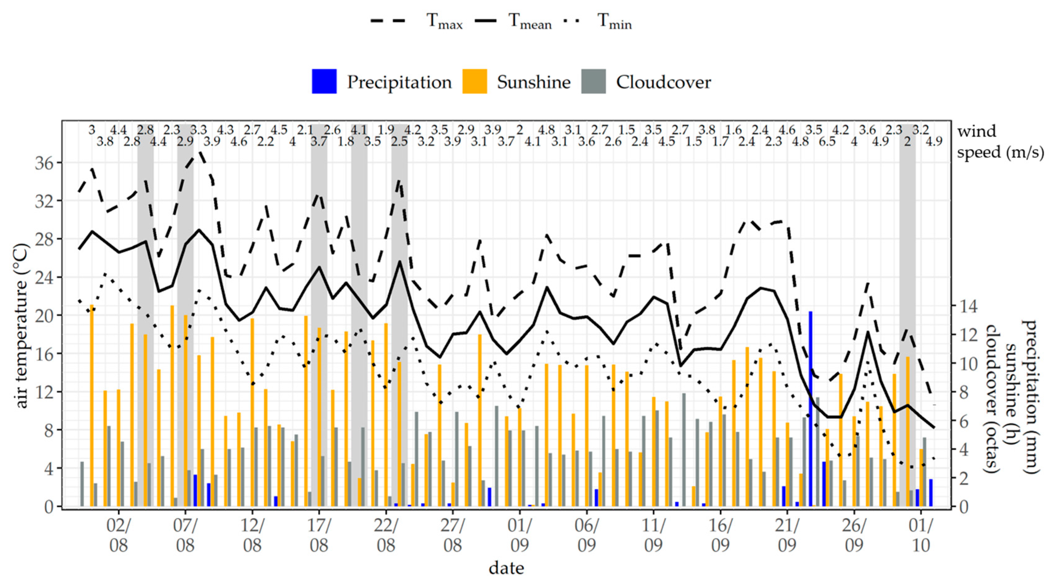
| (°C) | Precipitation (mm) | Cloud Cover (octas) | Sunshine (h) | Windspeed (m/s) | |
|---|---|---|---|---|---|
| Measurement period | 19.5 | 0.5 | 4.2 | 7.7 | 3.4 |
| All nights | 15.7 | 0.0 | 4.0 | 0.0 | 2.7 |
| Nights with calm and clear weather conditions | 18.1 | 0.0 | 1.0 | 0.0 | 2.7 |
© 2020 by the authors. Licensee MDPI, Basel, Switzerland. This article is an open access article distributed under the terms and conditions of the Creative Commons Attribution (CC BY) license (http://creativecommons.org/licenses/by/4.0/).
Share and Cite
Rost, A.T.; Liste, V.; Seidel, C.; Matscheroth, L.; Otto, M.; Meier, F.; Fenner, D. How Cool Are Allotment Gardens? A Case Study of Nocturnal Air Temperature Differences in Berlin, Germany. Atmosphere 2020, 11, 500. https://doi.org/10.3390/atmos11050500
Rost AT, Liste V, Seidel C, Matscheroth L, Otto M, Meier F, Fenner D. How Cool Are Allotment Gardens? A Case Study of Nocturnal Air Temperature Differences in Berlin, Germany. Atmosphere. 2020; 11(5):500. https://doi.org/10.3390/atmos11050500
Chicago/Turabian StyleRost, Annemarie Tabea, Victoria Liste, Corinna Seidel, Lea Matscheroth, Marco Otto, Fred Meier, and Daniel Fenner. 2020. "How Cool Are Allotment Gardens? A Case Study of Nocturnal Air Temperature Differences in Berlin, Germany" Atmosphere 11, no. 5: 500. https://doi.org/10.3390/atmos11050500
APA StyleRost, A. T., Liste, V., Seidel, C., Matscheroth, L., Otto, M., Meier, F., & Fenner, D. (2020). How Cool Are Allotment Gardens? A Case Study of Nocturnal Air Temperature Differences in Berlin, Germany. Atmosphere, 11(5), 500. https://doi.org/10.3390/atmos11050500