Spatial Mapping of a Highly Non-Uniform Distribution of Particle-Bound PAH in a Densely Populated Urban Area

Abstract

In this work, a 2-D gridded air pollution map with a high resolution of 50 × 50 m² was proposed to help the exposure assessment studies focusing on the association between air pollutants and their health effects. To establish a reliable air pollution map in a 2 × 2 km² urban area, a mobile monitoring procedure and a data process were developed. Among the various vehicle-related air pollutants, the particle-bound polycyclic aromatic hydrocarbon (pPAH) was chosen as a sensitive indicator. The average pPAH concentration on major roads (293.1 ng/m³) was found to be 35 times higher than that at a background location (8.4 ng/m³). Based on the cell-based pPAH concentrations, the 50 × 50 m² cells in the air pollution map were categorized into five pollution levels. The higher air pollution levels were generally shown by the cells close to the major traffic emission points. The proposed map can be used to make various policies regarding land use and traffic flow control in urban areas. Estimation of the personal exposure level to air pollutants is possible at a reliable location using the highly resolved 2-D gridded air pollution map in exposure assessment studies.

1. Introduction

In general, air quality is managed by monitoring criteria pollutants listed in the air quality standards at fixed stations. However, emissions from traffic is a dominant source of air pollutants in urban areas, which have a significant spatial difference in air pollution levels according to their proximity from roadways [1]. Because traffic hotspots are unevenly distributed in highly populated areas, air pollution near roadways is of great concern [2,3]. In addition, vehicles emit not only criteria pollutants but also other hazardous air pollutants (HAPs). In 2012, the International Agency for Research on Cancer (IARC) classified diesel engine exhaust as being carcinogenic to humans (Group 1) [4]. Due to the high toxicity of polycyclic aromatic hydrocarbons (PAHs), they have been widely studied among diesel engine exhaust [5,6,7].

Studies on the association between air pollutants and their adverse health effects have been conducted over decades [8]. These studies showed that air pollutants, such as nitrogen dioxide (NO₂), carbon monoxide (CO), particulate matters (PM₁₀, PM_2.5), black carbon (BC), and sulfur dioxide (SO₂), influence human health and increase the chances of respiratory, allergic, and cardiovascular diseases [9]. In particular, previous studies reported that the proximity to major roads in urban areas influenced the development of allergic diseases [10,11,12,13,14,15]. To conduct precise exposure assessments, air pollution data with a high spatial resolution are needed for urban areas [2].

To assess the levels of air pollutants in urban areas, the majority of studies used data from the nearest ambient air monitoring stations (AAMSs) [8]. However, due to the distance and the difference in surroundings between the location of interest and the AAMS, the accuracy of the predicted exposure levels has been somewhat questionable. This is especially significant when strong pollution sources, such as major roads with heavy traffic, are in the vicinity of the target location. In order to cope with these differences, researchers have applied numerical modeling techniques to accurately estimate air pollutant concentrations at the point of interest. Many regional-scale grid-based chemical transport models extensively used to simulate urban air quality have technical limitations upon reducing the horizontal grid size below 1 km [2]. Several regional/local-scale modeling approaches have tried to overcome such limitations [2]. These approaches include the probabilistic approach applying subgrid variability into a regional-scale model, the deterministic approach coupling a local-scale dispersion model with a regional-scale model, and the hybrid approach implementing a subgrid-scale treatment of the selected pollutant sources [16]. With regard to these approaches, source-based dispersion models have been popularly utilized in environmental health studies to provide more realistic distributions of air pollutant concentrations with strong spatial gradients [17].

To elucidate the non-uniform spatial distribution of air pollutants experimentally, various mobile measurements have been conducted using different platforms, such as pedestrians, bicycles, trams, and cars [18]. Among these, on-road measurements using a mobile laboratory (ML) have been popularly carried out. Westerdahl et al. (2005) demonstrated the great spatial distributions of ultrafine particles and the associated pollutant concentrations on freeways and residential streets in Los Angeles [19]. Further, in a 3 × 3 km² area, spatiotemporal CO and ultrafine particle concentrations were investigated by mobile monitoring [20]. Spatial distributions of traffic-related air pollutants were also characterized at a densely populated area in a mega city [6]. On-road mobile measurements could provide an NO_x profile around a signalized intersection of a busy roadway [21]. The spatial resolution of on-road measurements using an ML is much higher than that obtained through a regional-scale or even local-scale model. In a 4 × 4 km² area with a population density of 19,000/km², for example, regional-scale modeling, local-scale modeling, and mobile monitoring can provide air pollution data corresponding to 304,000, 760, and 48 populations, respectively (

Table 1. Comparison of spatial resolutions for three modeling/monitoring methods.

Method	Regional-Scale Modeling	Local-Scale Modeling	Mobile Monitoring
Spatial resolution	4 × 4 km2	200 × 200 m2	50 × 50 m2
Number of air pollution data in a 4 × 4 km2 area	1	400	6400
Population per air pollution data *	304,000	760	47.5

* Population density: 19,000/km².

). Therefore, mobile monitoring is a suitable method for examining the spatial distribution of air pollutant concentrations in an urban area with a high population density. The study area shows a high population density of 7th out of 226 local governments in Korea. Furthermore, a number of daycare centers, kindergartens, and schools are located in the study area. At the time of this study, we conducted “the Allergy & Gene-Environment Link (ANGEL) study” with Samsung Medical Center [22]. This hospital is located in the study area with many patients with allergic symptoms. In this project, we tried to link air pollutants with allergic symptoms, such as asthma and atopic dermatitis.

This study firstly established a two-dimensional (2-D) gridded air pollution map with a high resolution of 50 × 50 m² based on on-road mobile monitoring, which corresponds to the spatial-resolution requirement for traffic-related air pollutant exposure evaluations in epidemiological studies [23]. The air pollution map shows a greatly skewed distribution of vehicle-related air pollutants in a small part of an urban area. The mapping protocol for the 2-D gridded air pollution map is proposed, and then the spatial distribution of the particle-bound PAH (pPAH) concentration is analyzed and discussed.

2. Methods

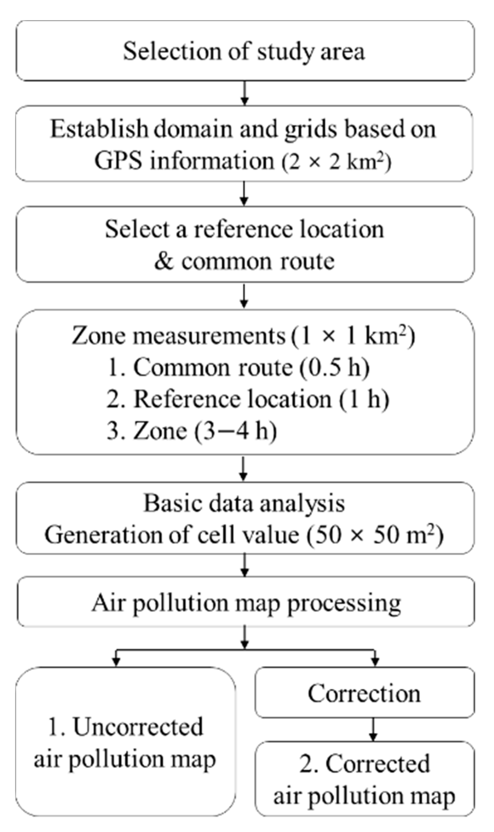
2.1. Mapping Protocol

A methodological framework is proposed for the 2-D gridded air pollution map with a high resolution based on on-road mobile monitoring (Figure 1). We considered a 2 × 2 km² domain divided into 1 × 1 km² zones, which were further divided into 50 × 50 m² cells. Here, a domain is the entire area of interest, a zone is the area covered by one-day measurements using an ML, and a cell is the spatial unit of the air pollution data. Prior to zone measurements, one-day preliminary measurement was carried out for screening non-accessible measurement routes in the entire domain. Overall measurement routes were determined according to the preliminary measurements. One-day zone measurements consisted of stationary measurements at a reference location, mobile measurements on a common route, and mobile measurements on a scripted route for each zone. A reference location was selected in a residential area adequately distanced from the busy roadways, such as the AAMS, to measure a background concentration during the monitoring period. A common route covering the entire domain was designed to measure the on-road concentration during the monitoring period. The background and common-route measurements were identically included in every zonal measurement. It is recommended that the measurement time is at least 1 h at the reference location, 0.5 h on the common route, and 3–4 h on the scripted route in the daytime after the morning rush hour on weekdays, minimizing the effects of on-road emission variability. After the overall measurements were completed, the measured time-series data were screened to adjust the response and delay times of instruments through a basic data analysis and allocated to 50 × 50 m² cells with global positioning system (GPS) information with a 1-s time interval. Cells with the number of 6-s measured data more than 10 were valid for inclusion in the air pollution map. The averages, standard deviations, and numbers were calculated for the data present in each valid cell.

Urban air pollution is influenced by many factors, such as meteorological and traffic conditions. Because the zone measurements are conducted over several consecutive days, day-to-day variations in air pollution levels are needed to be considered for establishing the air pollution map. In this study, we applied a simple correction method to correct the concentration of a pollutant measured on different days. The measured concentration (C_m) is corrected using:

C_c = C_m + (C_r(avg) − C_r(i)),

(1)

where C_c is the corrected concentration, C_r(avg) is the average concentration measured at the reference location over the entire measurement period, and C_r(i) is the concentration at the reference location on the ith day. As a result, the corrected air pollution map was obtained as the corrected concentrations were allocated to 50 × 50 m² cells following the procedure described above.

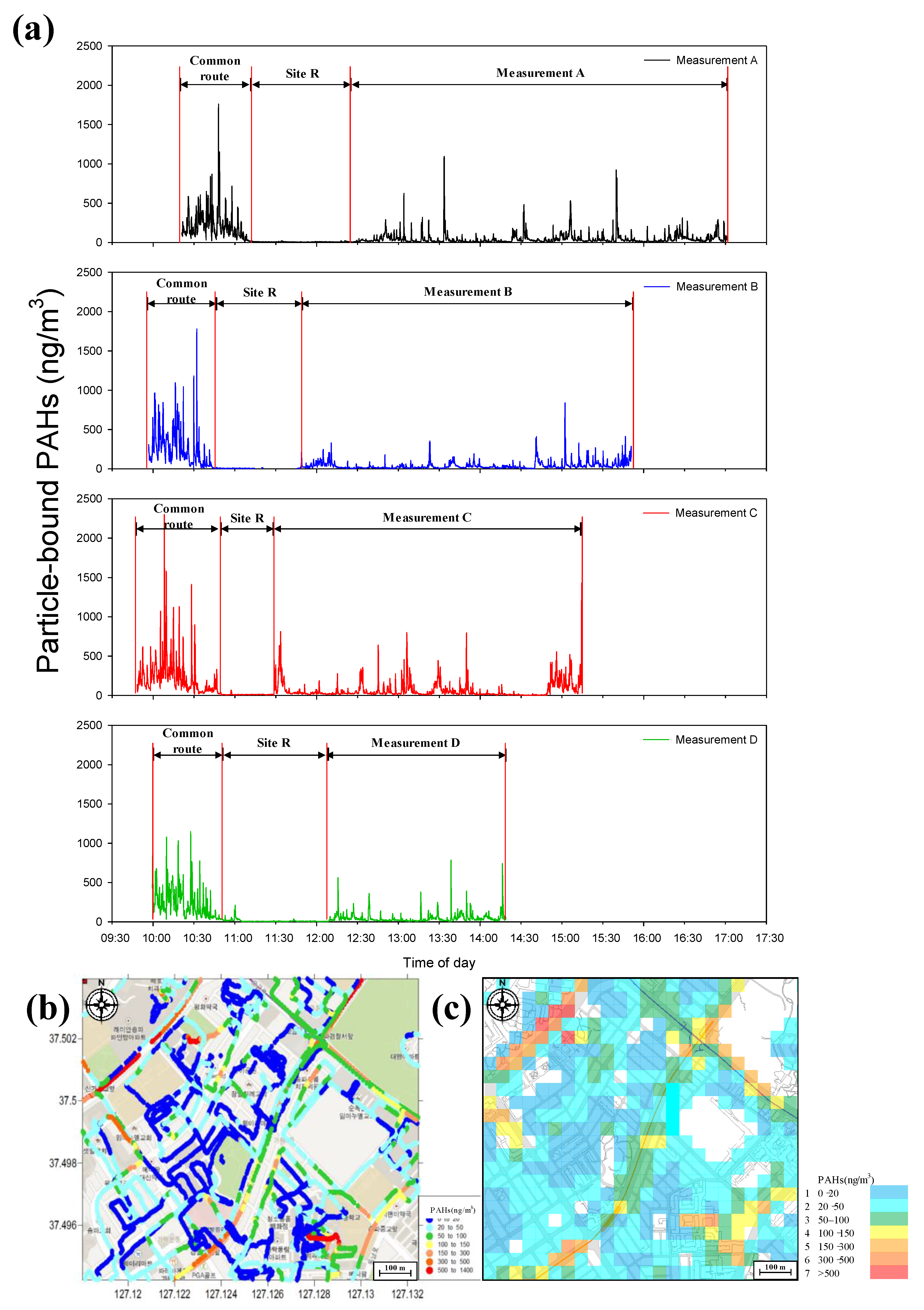
2.2. Mobile Monitoring

A 5-day measurement campaign from 9–13 June 2014 was carried out in a 2 × 2 km² domain in Songpa-gu district, Seoul, Republic of Korea. Figure 2a shows a map of Seoul consisting of 25 districts, with the Songpa-gu district being located in the southeastern part of Seoul. Songpa-gu district had the largest population of 677,460 in an area of 33.9 km² in the second quarter of 2014 [24]. The 2 × 2 km² domain was further divided into 1 × 1 km² sub-domains (zones A, B, C, and D), as shown in Figure 2b. The reference location was selected in the Olympic Park and the common route was designed to include major roads in the Songpa-gu district (Figure 2c). Olympic Park was selected as a reference site since the air quality monitoring station (AQM) is located and it is surrounded by green area where the background level could be measured as shown in Figure 2c. The scripted routes for the zone measurements were designed to ensure maximum spatial coverage of all accessible roads in the entire domain (Figure 2d). The measurement times were approximately during 10:00 a.m.–04:00 p.m., following the recommendation of the mapping protocol. The mobile measurements on the common route and the stationary measurements at the reference location were conducted approximately during 10:00 a.m.–11:00 a.m. and 11:00 a.m.–12:00 p.m., respectively, for all 5 days. The zone measurements were carried out during 12:00 p.m.–16:00 p.m. from 10–13 June (4 days). According to statistics, there was no significant change in the traffic volume between 10:00 a.m. and 16:00 p.m. on weekdays in Songpa-gu district [24]. In the mapping process based on the GPS information, 1227 (77%) out of the 1600 cells in the 2 × 2 km² domain matched with the scripted routes, which could be visualized in the 2-D gridded air pollution map. The rest of the 373 cells were the spaces where the ML could not be accessible or where insufficient numbers of measured data, i.e., less than 10, were obtained. The numbers of valid cells in zones A, B, C, and D range from 242 (61%) to 335 (84%), while more than 10,000 data measurements were collected for all zones except for zone D.

Air pollutant concentrations were measured using the ML following the measurement protocol designed by the combination of mobile and stationary measurements using an ML [6]. The sampling inlets of an ML are a stainless-steel pipe and a Teflon tubing for collecting particulate and gaseous pollutants, respectively. The sampling height was approximately 2 m above the ground level. The ML was equipped with a PAH monitor with a photoelectric aerosol sensor (PAS 2000, EcoChem, League City, TX, USA) to measure the pPAH concentration. A pPAH with three or more benzene rings is detected through the measurement of the electrons emitted by organic molecules on particles irradiated by UV light. Thus, we could only quantify the total concentration of pPAH that has photo-electric activity. The sampling air flow rate of the PAH monitor was set at 2.0 L/min, and a lamp with a wavelength of 220 nm was set to turn off for 2 s for the background measurement and then turn on for 4 s for the sample measurement. The measurement time of the PAH monitor was synchronized with the GPS time before starting the measurement every day.

3. Results and Discussion

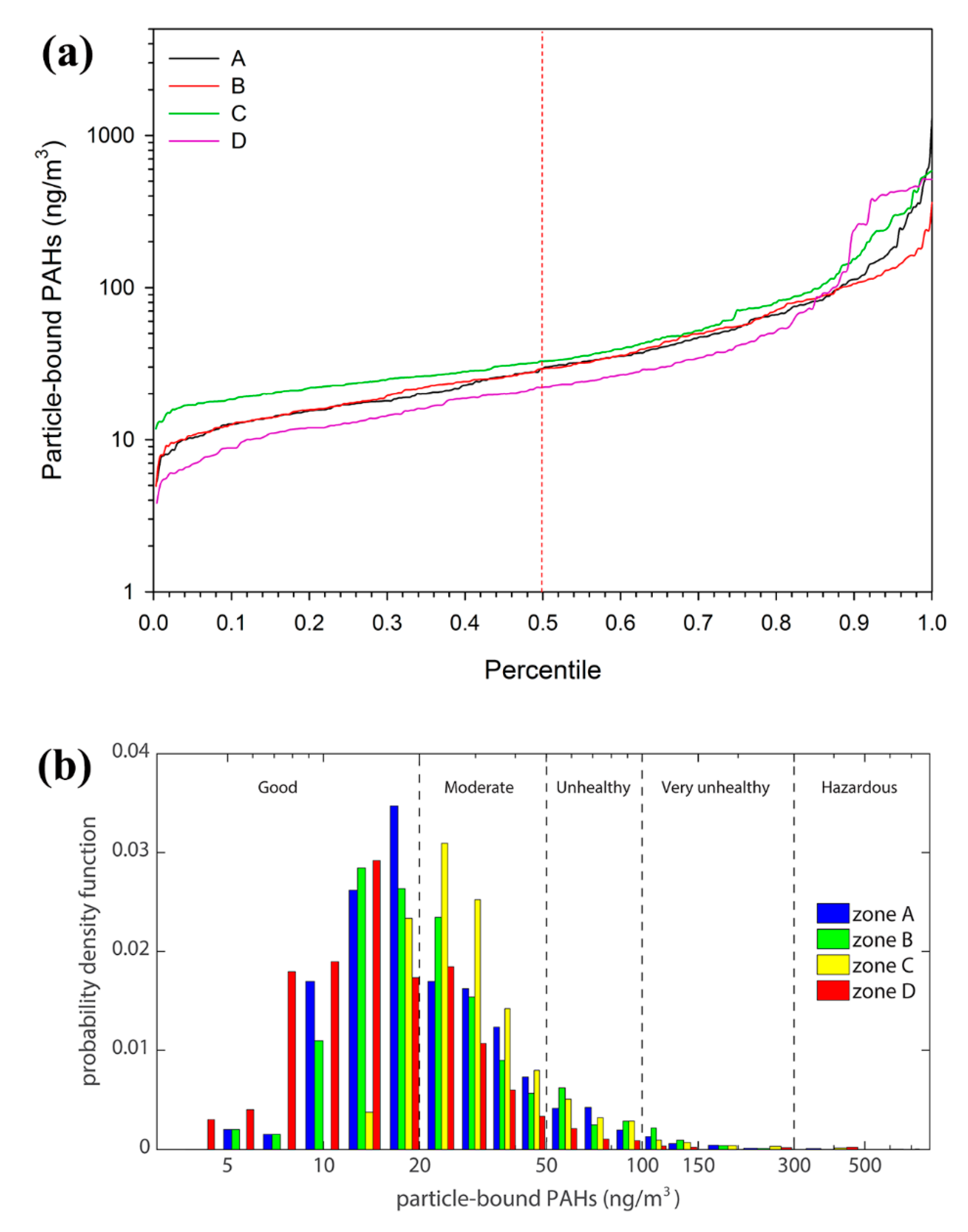
3.1. Zone- and Cell-Based Analysis

Table 2. Date and time of measurements and the pPAH concentrations at (a) the reference location and (b) the common route (unit: ng/m³).

Classification	Preliminary Measurement	Zone Measurements
(a) Reference location Measurement date and time	11:30–12:26 9 June	11:15–12:39 10 June	10:43–11:47 11 June	10:49–11:26 12 June	11:07–12:06 13 June
Average ± standard deviation	9.4 ± 5.8	9.7 ± 6.7	6.2 ± 4.7	11.2 ± 6.6	5.3 ± 2.1
(b) Common route Measurement date and time	13:02–13:23 9 June	10:21–10:41 10 June	09:56–10:16 11 June	09:49–10:10 12 June	10:00–10:22 13 June
Average ± standard deviation	255.0 ± 220.5	245.3 ± 134.1	333.4 ± 195.5	315.6 ± 272.7	316.2 ± 164.3

shows the actual 5-day measurement schedule, which we designed and carried out. The number of data points are shown in

Table 3. Zone- and cell-based statistical analysis of pPAH concentrations over a 2 × 2 km² domain.

Classification		Zone A	Zone B	Zone C	Zone D
Zone-based (1 × 1 km2)	Number of valid data (n)	12,583	10,372	10,304	6419
	Average (ng/m3)	57 ± 106	42 ± 43	70 ± 82	95 ± 159
	Median (ng/m3)	29	28	35	29
	5% (ng/m3)	10	10	18	10
	25% (ng/m3)	17	17	25	18
	75% (ng/m3)	53	51	74	68
	95% (ng/m3)	179	118	266	532
Cell-based (50 × 50 m2)	Number of valid data (n/km2)	12,120	9906	8214	5903
	Number of valid cells (/km2)	334	316	335	242
	Average (ng/m3)	58 ± 106	46 ± 45	69 ± 97	67 ± 121
	Median (ng/m3)	30	29	33	22
	5% (ng/m3)	10	11	17	7
	25% (ng/m3)	17	17	23	13
	75% (ng/m3)	55	56	71	42
	95% (ng/m3)	182	135	292	424
Meteorological variables	Wind speed (m/s)	1.6 ± 0.6	2.4 ± 0.5	1.8 ± 0.4	2.1 ± 0.4
	Prevailing wind direction	NW, SE	NE	SE	NW
	Temperature (°C)	27.2 ± 0.4	27.2 ± 1.9	23.9 ± 2.2	25.5 ± 0.9
	Relative humidity (%)	70.8	72	87.1	73.9

for the zone A, B, C, and D. The measurement schedule and the time of data collection were strictly maintained during the whole measurements and the driver of the mobile laboratory always kept the same researcher for data collection consistency. For the data comparison, the nearest AQM (Figure 2c) data were obtained and compared but only NO₂ could be comparable with the mobile measurement data, showing a 0.88 of the coefficient of determination (r²).

Among the concentrations of several particulate and gaseous pollutants measured by the instruments installed in the ML during the 5-day measurement period, the pPAH concentration was chosen for establishing the 2-D gridded air pollution map. A time-series of pPAH concentrations during the 4-day measurement period is shown in Figure 3a. The pPAH concentrations with a 6-s interval were combined with the data obtained from the GPS, resulting in a 1-D line-type air pollution map, as shown in Figure 3b, for zone A. In the mapping process, the pPAH concentrations were allocated into 50 × 50 m² cells to establish a 2-D gridded air pollution map, as shown in Figure 3c, for zone A.

Table 2 summarizes the pPAH concentrations measured at the reference location and on the common route for five days. At the reference location, the average pPAH concentration ranges from 5.3 (zone D) to 11.2 (zone C) ng/m³. Over the 5-day measurement, the average and the coefficient of variation (CV) of the pPAH concentration are 8.4 ng/m³ and 6.2%, respectively. On the common route, the average pPAH concentration ranges from 245.3 (zone A) to 333.4 (zone B) ng/m³. Over the 5-day measurement, the average and the CV of the pPAH concentration are 281.6 ng/m³ and 215.7%, respectively. The average pPAH concentration on the common route is 31 times higher than that at the reference location, implying the traffic emissions are the major sources of measured pPAH in the all the zones.

The statistics for the measured pPAH concentrations and meteorological variables for zones A, B, C, and D are listed in Table 3. The meteorological variables were observed at the automatic weather station (AWS) in Songpa-gu district, which is located about 1–3 km from the selected domain of this study (Figure 2c). Prevailing winds blew from northwest (NW)-to-southeast (SE), northeast (NE), SE, and NW in the zone A, B, C, and D measurements, respectively. The frequencies of 1-min averaged wind speeds showed that wind speeds smaller than 1.5 m/s accounted for 21%, wind speeds ranging from 1.5 to 2.5 m/s accounted for 70%, and wind speeds larger than 2.5 m/s accounted for 9%.

First, a zone-based analysis was conducted. The results showed the average pPAH concentrations range from 42 (zone B) to 95 (zone D) ng/m³. In contrast, the median pPAH concentrations ranged from 28 (zone B) to 35 (zone C) ng/m³, which are significantly lower than the average concentrations for all zones. The spatial distribution of the pPAH concentration was found to be skewed toward higher concentrations. The highest average (zone D) and median (zone C) concentrations were not found in the same zone. In addition, for example, the 95% pPAH concentration is 18 times higher than the median concentration for zone D, whereas it is only 4.2 times higher than the median pPAH concentration for zone B.

Second, a cell-based analysis was conducted during the mapping process. Due to the valid-cell criteria, some data used in the zone-based analysis were discarded. Effective cells obtained from mobile monitoring over the entire domain are shown in Figure 4b,c. As it can be seen, the average pPAH concentration ranges from 46 (zone B) to 69 (zone C) ng/m³ and their average is 60 ng/m³, whereas the median pPAH concentration ranges from 22 (zone D) to 33 (zone C) ng/m³ and their average is 28.5 ng/m³. On average, the average and median pPAH concentrations were 7 and 3.4 times higher than the pPAH concentration at the reference location. Note that the average and the 95% concentrations were significantly decreased for zone D compared to those for the other zones. In the cell-based analysis, peak concentrations were smoothed because these were removed when the concentration of cells was calculated. Thus, it is concluded that cell-based air pollution data may be more reliable due to a reduction of the inevitable short disturbance effects due to plumes during on-road mobile measurements.

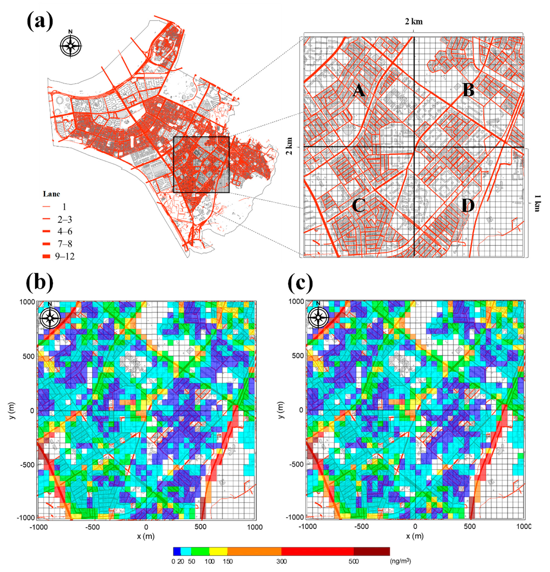
3.2. Spatial Distribution in the Air Pollution Map

The 2-D gridded air pollution map and the distribution of roads with the number of lanes in the 2 × 2 km² domain are shown in Figure 4. Considering the average pPAH concentrations at the reference location are below 11 ng/m³ and the median cell-based pPAH concentrations are below 33 ng/m³, 50 × 50 m² cells were categorized into five pollution levels based on the cell-based pPAH concentrations. The selected pollution levels were ‘good’ (<20 ng/m³), ‘moderate’ (20–50 ng/m³), ‘unhealthy’ (50–100 ng/m³), ‘very unhealthy’ (100–300 ng/m³), and ‘hazardous’ (>300 ng/m³). The corrected air pollution map using Equation (1) is shown in Figure 4c. Note that the maximum difference between C_r(avg) and C_r(i) is only 3.1 ng/m³ because the pPAH concentrations at the reference location are relatively low (5–11 ng/m³).

Among the various land-use categories, residential areas accounted for the largest portion in the 2 × 2 km² domain. Most residential areas (68–79%) were categorized under the ‘good’ or ‘moderate’ level, indicating the pPAH concentrations to be below 50 ng/m³ in these areas. On the other hand, the majority of residential areas close to the main arterial roads were categorized under the ‘unhealthy’ level, indicating the pPAH concentration is in the range of 50–100 ng/m³, and suggesting that the residents living within 100–200 m from the major roadways could be exposed to elevated pPAH concentrations. The cells marked for higher pollution levels were mainly shown along the major arterial roadways and the express motorway. Interestingly, the signalized intersection areas exhibited more elevated pPAH concentrations than the roadways on the connecting routes. Kim et al. (2014) reported an aggravation in the air pollution levels around a signalized intersection area resulting from increased emissions due to transient driving patterns [21]. A large spatial gradient of the pollutant concentration exponentially decreasing with an increasing distance from the major roadways has been reported in several studies [1,5,25,26,27]. Therefore, it can be said that traffic emissions are major source of pPAH in the study area, especially in the vicinity of major roadways.

Statistics on the pPAH concentrations for the five pollution levels are summarized in

Table 4. Number of cells categorized into five levels of pPAH concentrations for zones A, B, C, and D.

Pollution Level	Zone A	Zone B	Zone C	Zone D
Good (pPAH ≤ 20 ng/m3)	115/124 * (34.4/37.1%)	98/84 (31.0/26.6%)	49/59 (14.6/17.6%)	110/86 (45.5/35.5%)
Moderate (20 < pPAH ≤ 50 ng/m3)	127/119 (38.0/35.6%)	125/133 (39.6/42.1%)	180/175 (53.7/52.2%)	82/102 (33.9/42.1%)
Unhealthy (50 < pPAH ≤ 100 ng/m3)	52/51 (15.6/15.3%)	56/61 (17.7/19.3%)	57/52 (17.0/15.5%)	19/22 (7.9/9.1%)
Very unhealthy (100 < pPAH ≤ 300 ng/m3)	29/29 (8.7/8.7%)	36/37 (11.4/11.7%)	34/34 (10.1/10.1%)	11/12 (4.5/5.0%)
Hazardous (pPAH > 300 ng/m3)	11/11 (3.3/3.3%)	1/1 (0.3/0.3%)	15/15 (4.5/4.5%)	20/20 (8.3/8.3%)

* Uncorrected/corrected.

. The cells categorized into ‘unhealthy’, ‘very unhealthy’, or ‘hazardous’ levels occupy 28%, 29%, 32%, and 21% in the uncorrected air pollution map for zones A, B, C, and D, respectively, whereas they occupy 27%, 31%, 30%, and 22% in the corrected air pollution map for zones A, B, C, and D, respectively. Compared with other zones, zone D has the smallest portion of ‘unhealthy’, ‘very unhealthy’, or ‘hazardous’ levels in relation to the relatively sparse distribution of roadways. As mentioned in Figure 4, these polluted cells are distributed mostly within 200 m from the roadways.

The cumulative distributions and probability density functions (PDFs) of cell-based pPAH concentrations in zones A, B, C, and D are shown in Figure 5. The PDF of the pPAH concentration is the number of cells in the specified concentration range divided by the total number of cells and by the width of the concentration range. In other words, the summation of PDF multiplied by the width of the concentration range is unity. The four cumulative distributions seem to be similar to each other except for those in the range of concentrations higher than 100 ng/m³. The lowest concentration at a certain percentile (up to 85 percentile) was consistently found in zone D followed by zone A or B. In contrast, the concentration in zone D was the highest at the 90–97 percentile, followed by those in zone C, A, and B, which is consistent with the largest portion of the ‘hazardous’ level in zone D (8%) (Table 4). The data on PDFs reveal that most of the cells are concentrated at 11–15 ng/m³ (zones B and D), 15–20 ng/m³ (zone A), and 20–26 ng/m³ (zone C). It is clear that the PDF in zone D shows a shift toward lower concentrations compared with those in other zones, which is consistent with the largest portion of the ‘good’ level in zone D (46%) (Table 4). Consequently, the pPAH concentration in zone D showed the highest diversity from the ‘good’ to ‘hazardous’ levels among the four zones. The ‘good’ level was attributed to the relatively sparse distribution of roadways and the ‘hazardous’ level to the express motorway in zone D.

Despite our efforts on the study design and results, this study has several limitations. First, our zone measurements were carried out from 12:00 p.m. to 16:00 p.m. during the weekday in order to avoid the significant changes in traffic volume. More measurements on weekends and other time periods during weekdays, such as rush hour, should be carried out to provide a much more significant spatial distribution for the study area. Second, similar measurements have to be carried out for other seasons to provide seasonal variability to the exposure assessments. More spatial and temporal variation of the changes in air pollutants would provide more reliable data to link with an estimate of the prevalence for persons affected by allergies for the study area. Third, a highly resolved PM_2.5 spatial distribution should be conducted further because a previous study in New York showed the PM_2.5-attributable deaths, hospitalization, and emergency department visits in an urban area [28]. Our study could not provide the PM_2.5 mass concentration due to the technical difficulties in the iso-kinetic sampling of PM_2.5 while driving due to the speed of the mobile laboratory. This could be overcome by the improvement of the link from the flow rate of the sampling blower and the vehicle speed.

4. Conclusions

Mapping the spatial distribution of air pollution at a high resolution is a major requirement for air quality management in a densely populated urban area. In this study, we firstly established a 2-D gridded air pollution map with a resolution of 50 × 50 m² based on on-road mobile monitoring. Following the proposed mapping protocol using an ML, mobile and stationary measurements were taken over a 2 × 2 km² domain during five consecutive weekdays. Among various traffic-related air pollutants, pPAH was selected as an indicator of vehicle emission. The measured pPAH concentrations were allocated to 50 × 50 m² cells using GPS information. In the statistical analysis, the average cell-based pPAH concentration (60 ng/m³) was about 7 times higher than the average pPAH concentration (8.4 ng/m³) at the reference location. The 50 × 50 m² cells in the air pollution map were categorized into five pollution levels (i.e., ‘good’, ‘moderate’, ‘unhealthy’, ‘very unhealthy’, and ‘hazardous’) on the basis of their pPAH concentrations that are reliable for representing air pollution levels. Residential areas close to main arterial roads (within 200 m) were found to be exposed to ‘unhealthy’ or higher levels of pPAH concentration. One 1 × 1 km² zone, characterized by sparsely distributed roadways and express motorways, accounted for the largest portions of both ‘good’ and ‘hazardous’ levels. We reached a firm conclusion that traffic emission is primarily attributed to elevated pollution levels resulting in hotspots in residential areas close to roadways.

A highly non-uniform spatial distribution of air pollution levels in an urban area could be visualized through the established high-resolution air pollution map. Using this air pollution map, exposure to air pollutants can be estimated at the individual level for a close and reasonable location in exposure assessment studies. The reliability of cell-based concentrations needs to be investigated through further studies considering seasonal differences, various air pollutants, and influencing key factors. We plan to compare a hybrid model with regional- and local-scale models in our future works.

References

1. Hitchins, J.; Morawska, L.; Wolff, R.; Gilbert, D. Concentrations of submicrometre particles from vehicle emissions near a major road. Atmos. Environ. 2000, 34, 51–59. Available online: http://www.sciencedirect.com/science/article/pii/S1352231099003040 (accessed on 27 October 1999). [CrossRef] [Green Version]
2. Touma, J.S.; Isakov, V.; Ching, J.; Seigneur, C. Air quality modeling of hazardous pollutants: Current status and future directions. J. Air Waste Manag. Assoc. 2006, 56, 547–558. [Google Scholar] [CrossRef] [PubMed] [Green Version]
3. Joint, W.H.O.; World Health Organization. Health Risks of Particulate Matter from Long-Range Transboundary Air Pollution; WHO Regional Office for Europe: Copenhagen, Denmark, 2006. [Google Scholar]
4. IARC. Iarc: Diesel Engine Exhaust Carcinogenic. 2012. Available online: https://www.iarc.fr/en/media-centre/pr/2012/pdfs/pr213_E.pdf (accessed on 12 June 2012).
5. Kim, K.H.; Lee, S.B.; Woo, D.; Bae, G.N. Influence of wind direction and speed on the transport of particle-bound PAHs in a roadway environment. Atmos. Pollut. Res. 2016, 6, 1024–1034. Available online: http://www.sciencedirect.com/science/article/pii/S1309104215000148 (accessed on 21 October 2015). [CrossRef]
6. Kim, K.H.; Woo, D.; Lee, S.B.; Bae, G.N. On-road measurements of ultrafine particles and associated air pollutants in a densely populated area of Seoul, Korea. Aerosol Air Q. Res. 2015, 15, 142–153. [Google Scholar] [CrossRef] [Green Version]
7. Houston, D.; Wu, J.; Yang, D.; Jaimes, G. Particle-bound polycyclic aromatic hydrocarbon concentrations in transportation microenvironments. Atmos. Environ. 2013, 71, 148–157. Available online: http://www.sciencedirect.com/science/article/pii/S135223101300099X (accessed on 13 February 2013). [CrossRef]
8. Lee, J.Y.; Lee, S.-B.; Bae, G.-N. A review of the association between air pollutant exposure and allergic diseases in children. Air Pollut. Res. 2014, 5, 616–629. [Google Scholar] [CrossRef] [Green Version]
9. Zanobetti, A.; Luttmann-Gibson, H.; Horton, E.S.; Cohen, A.; Coull, B.A.; Hoffmann, B.; Schwartz, J.D.; Mittleman, M.A.; Li, Y.; Stone, P.H.; et al. Brachial artery responses to ambient pollution, temperature, and humidity in people with type 2 diabetes: A repeated-measures study. Environ. Health Perspect. 2014, 122, 242–248. [Google Scholar] [CrossRef] [Green Version]
10. Guo, Y.L.; Lin, Y.C.; Sung, F.C.; Huang, S.L.; Ko, Y.C.; Lai, J.S.; Su, H.J.; Shaw, C.K.; Lin, R.S.; Dockery, D.W. Climate, traffic-related air pollutants, and asthma prevalence in middle-school children in Taiwan. Environ. Health Perspect. 1999, 107, 1001–1006. Available online: http://www.ncbi.nlm.nih.gov/pmc/articles/PMC1566819/ (accessed on 17 November 1999). [CrossRef] [Green Version]
11. Venn, A.; Lewis, S.; Cooper, M.; Hubbard, R.; Britton, J. Living near a main road and the risk of wheezing illness in children. Am. J. Respir. Crit. Care Med. 2001, 164, 2177–2180. [Google Scholar] [CrossRef]
12. Lee, Y.L.; Su, H.J.; Sheu, H.M.; Yu, H.S.; Guo, Y.L. Traffic-related air pollution, climate, and prevalence of eczema in Taiwanese school children. J. Invest. Dermatol. 2008, 128, 2412–2420. [Google Scholar] [CrossRef]
13. Jerrett, M.; Shankardass, K.; Berhane, K.; Gauderman, W.J.; Kunzli, N.; Avol, E.; Gilliland, F.; Lurmann, F.; Molitor, J.N.; Molitor, J.T.; et al. Traffic-related air pollution and asthma onset in children: A prospective cohort study with individual exposure measurement. Environ. Health Perspect. 2008, 116, 1433–1438. [Google Scholar] [CrossRef] [PubMed] [Green Version]
14. Cook, A.G.; de Vos, A.J.; Pereira, G.; Jardine, A.; Weinstein, P. Use of a total traffic count metric to investigate the impact of roadways on asthma severity: A case-control study. Environ. Health 2011, 10, 52. [Google Scholar] [CrossRef] [PubMed] [Green Version]
15. Morgenstern, V.; Zutavern, A.; Cyrys, J.; Brockow, I.; Koletzko, S.; Kramer, U.; Behrendt, H.; Herbarth, O.; von Berg, A.; Bauer, C.P.; et al. Atopic diseases, allergic sensitization, and exposure to traffic-related air pollution in children. Am. J. Respir. Crit. Care Med. 2008, 177, 1331–1337. [Google Scholar] [CrossRef] [PubMed]
16. Stein, A.F.; Isakov, V.; Godowitch, J.; Draxler, R.R. A hybrid modeling approach to resolve pollutant concentrations in an urban area. Atmos. Environ. 2007, 41, 9410–9426. Available online: http://www.sciencedirect.com/science/article/pii/S1352231007007881 (accessed on 14 September 2007). [CrossRef]
17. Isakov, V.; Touma, J.S.; Burke, J.; Lobdell, D.T.; Palma, T.; Rosenbaum, A.; Ozkaynak, H. Combining regional- and local-scale air quality models with exposure models for use in environmental health studies. J. Air Waste Manag. Assoc. 2009, 59, 461–472. [Google Scholar] [CrossRef]
18. Van den Bossche, J.; Peters, J.; Verwaeren, J.; Botteldooren, D.; Theunis, J.; de Baets, B. Mobile monitoring for mapping spatial variation in urban air quality: Development and validation of a methodology based on an extensive dataset. Atmos. Environ. 2015, 105, 148–161. Available online: http://www.sciencedirect.com/science/article/pii/S1352231015000254 (accessed on 8 January 2015). [CrossRef] [Green Version]
19. Westerdahl, D.; Fruin, S.; Sax, T.; Fine, P.M.; Sioutas, C. Mobile platform measurements of ultrafine particles and associated pollutant concentrations on freeways and residential streets in Los Angeles. Atmos. Environ. 2005, 39, 3597–3610. [Google Scholar] [CrossRef]
20. Hagler, G.S.; Thoma, E.D.; Baldauf, R.W. High-resolution mobile monitoring of carbon monoxide and ultrafine particle concentrations in a near-road environment. J. Air Waste Manag. Assoc. 2010, 60, 328–336. [Google Scholar] [CrossRef]
21. Kim, K.H.; Lee, S.-B.; Woo, S.H.; Bae, G.-N. NOx profile around a signalized intersection of busy roadway. Atmos. Environ. 2014, 97, 144–154. Available online: http://www.sciencedirect.com/science/article/pii/S1352231014006062 (accessed on 4 August 2014). [CrossRef]
22. Kim, Y.-M.; Kim, J.; Han, Y.; Lee, B.-J.; Choi, D.-C.; Cheong, H.-K.; Jeon, B.-H.; Oh, I.; Bae, G.-N.; Lee, J.Y.; et al. Comparison of diverse estimation methods for personal exposure to air pollutants and associations with allergic symptoms: The allergy & gene-environment link (angel) study. Sci. Total Environ. 2017, 579, 1127–1136. Available online: http://www.sciencedirect.com/science/article/pii/S0048969716325281 (accessed on 30 November 2016). [CrossRef]
23. Batterman, S.; Chambliss, S.; Isakov, V. Spatial resolution requirements for traffic-related air pollutant exposure evaluations. Atmos. Environ. 2014, 94, 518–528. Available online: http://www.sciencedirect.com/science/article/pii/S1352231014004312 (accessed on 26 May 2014). [CrossRef] [PubMed] [Green Version]
24. Government, S.M. Seoul Statistical Yearbook; Seoul Metropolitan Government: Seoul, Korea, 2014.
25. Hagler, G.S.W.; Baldauf, R.W.; Thoma, E.D.; Long, T.R.; Snow, R.F.; Kinsey, J.S.; Oudejans, L.; Gullett, B.K. Ultrafine particles near a major roadway in Raleigh, North Carolina: Downwind attenuation and correlation with traffic-related pollutants. Atmos. Environ. 2009, 43, 1229–1234. Available online: http://www.sciencedirect.com/science/article/pii/S1352231008010832 (accessed on 30 November 2008). [CrossRef]
26. Zhu, Y.; Hinds, W.; Kim, S.; Sioutas, C. Concentration and size distribution of ultrafine particles near a major highway. J. Air Waste Manag. Assoc. 2002, 52, 1032–1042. [Google Scholar] [CrossRef] [PubMed]
27. Zhu, Y.; Hinds, W.; Kim, S.; Shen, S.; Sioutas, C. Study of ultrafine particles near a major highway with heavy-duty diesel traffic. Atmos. Environ. 2002, 36, 4323–4335. [Google Scholar] [CrossRef]
28. Kheirbek, I.; Haney, J.; Douglas, S.; Ito, K.; Matte, T. The contribution of motor vehicle emissions to ambient fine particulate matter public health impacts in New York City: A health burden assessment. Environ. Health 2016, 15, 89. [Google Scholar] [CrossRef] [Green Version]
Figure 1. Flow chart of the methodological framework for the 2-D gridded air pollution map.
Atmosphere 11 00496 g001
Figure 2. (a) Map of Seoul, (b) study area, (c) common route, and (d) 4-day measurement routes with zones A, B, C, and D. The reference location is indicated as a red circle and the common route is shown using blue dotted lines. Detailed traveling routes are presented with different colors for each day.
Atmosphere 11 00496 g002
Figure 3. (a) Processing of a time-series data, (b) line map, and (c) 2-D map for pPAH.
Atmosphere 11 00496 g003
Figure 4. (a) Roadway map and study domain in Songpa-gu district. (b) Uncorrected and (c) corrected 2-D gridded air pollution map with seven pPAH concentration levels.
Atmosphere 11 00496 g004
Figure 5. (a) Cumulative distributions and (b) probability density functions of cell-based pPAH concentrations for zone A, B, C, and D. The number of concentration ranges in the probability density functions is 22.
Atmosphere 11 00496 g005