A Wind Tunnel Investigation into the Aerodynamics of Lobed Hailstones

Abstract

The complex surface geometries of hailstones affect their fall behavior, fall speeds, and growth. Systematic experimental investigations on the influence of the number and length of lobes on the fall velocity and the drag coefficient of hailstones were performed in the Mainz vertical wind tunnel to provide relationships for use in numerical models. For this purpose, 3D prints of four artificial lobed hailstone models as well as spheres were used. The derived drag coefficients show no dependency in the Reynolds number in the range between 25,000 and 85,000. Further, the drag coefficients were found to increase with increasing length of lobes. All lobed hailstones show higher or similar drag coefficients than spheres. The terminal velocities of the the hailstones with short lobes are very close to each other and only reduced by about 6% from those of a sphere. The terminal velocities from the long lobed hailstones deviate up to 21% from a sphere. The results indicate that lobes on the surface of hailstones reduce their kinetic energy by a factor of up to 3 compared to a sphere. This has important consequences for the estimation of the destructive potential of hailstones.

1. Introduction

According to the fifth assessment report of the IPCC, and e.g., Lehmann et al. [1] as well as Brimelow et al. [2], extreme precipitation events are very likely to increase in rate and frequency in the next decades due to climate change. Hailstorms are among the most destructive extreme weather events in several regions all over the world, causing substantial damage to crops, vehicles, buildings and other infrastructures. Hence, there is an urgency to accelerate the research on hail in order to reliably predict and thereby reduce the damage from hailstorms.

According to the World Meteorological Organization International Cloud Atlas hailstones are heavily rimed ice particles which are larger than 5 $\mathrm{mm}$ in diameter. Smaller ones are called graupel. Typically, the diameters of hailstones range between 5 $\mathrm{mm}$ and 50 $\mathrm{mm}$. While small hailstones have densities of about $0.5$ $\mathrm{g}$ ${\mathrm{cm}}^{\mathrm{-3}}$ [3] large hailstones have densities higher than $0.8$ $\mathrm{g}$ ${\mathrm{cm}}^{\mathrm{-3}}$, because any internal hollows fill up with water as the hailstones are transported into temperature regimes above 0 ${}^{\circ }\mathrm{C}$. Thus, a major factor influencing the density is the growth regime. During dry-growth, the latent heat from the freezing of the colliding droplets is transported to the environmental air fast enough so that the surface temperature is well below 0 ${}^{\circ }\mathrm{C}$, i.e., there is no liquid water on the hailstone surface. This produces opaque low-density rime ice caused by air bubbles incorporated in the interstice of the frozen droplets [4,5]. In contrast, wet-growth occurs when surface temperatures are close to 0 ${}^{\circ }\mathrm{C}$. i.e., at higher ambient temperatures and/or at high liquid water contents. During wet-growth the water freezes rather transparent and is called spongy ice. The shapes of hailstones can be conical, spheroidal or irregular with spikes and lobes on the surface [6,7,8] and are influenced by various factors. Hail initiated by a conical graupel is rather conical whereas hail initiated by a frozen drop grows rather spherically. There are two types of lobes on hailstones; crusped lobes and icicle lobes [9,10]. Crusped lobes are formed in a dry-growth regime. It is a collection efficiency effect which includes a tumbling fall behavior. If a hailstone tumbles during its fall, the droplets collide at the protrusions and shield the valleys from further growth [9]. Icicle lobes instead are generated from a composite effect including the collection efficiency effect and the ventilation effect and occurs in the wet-growth regime. The ventilation effect is a factor describing the enhancement of heat and mass transfer to or from the surface of a falling hydrometeor compared to a pure diffusive case. This effect causes the liquid water to freeze more efficiently at the tips of protrusions due to an increased heat transfer. Hydrodynamic forces might also contribute to the growth of the icicle lobes [9]. In general, icicle lobes show more distinct surface features than crusped lobes. Furthermore, among other factors, the lobes affect the mass and heat transfer to or from the surface of a hailstone, i.e., a hailstone which falls into a subsaturated airmass consumes the heat from its environment and cools the surrounding air. This cooling causes the downburst phenomenon, which is responsible for substantial damages at the ground. Wang and Chueh [11] found that the ventilation effect for large lobed hailstones is increased by a factor of up 2.5 compared to spheres of the same size. The developing lobes in turn affect the flow field around the hailstones (e.g., Wang et al. [12] and Cheng and Wang [13]), and thus their fall characteristics such as drag coefficient, terminal velocity, and fall behavior.

From the above explanation it is obvious that the growth mechanism of a hailstone, i.e., the capability of a hailstone to collect supercooled droplets, and the fall characteristics are closely related. Finally, this interplay determines the mass and the terminal velocity of a hailstone. Both quantities are essential for estimating the kinetic energy, and thus the destructive potential of a hailstone at the ground. Therefore, a correct understanding of the influence of lobes on the fall properties of hailstones such as fall mode, terminal velocity and drag coefficient is crucial to reliably simulate the growth of hailstones with numerical models. Wang et al. [12] performed numerical simulations on the flow fields around lobed hailstones to investigate their influence on the drag coefficient. For that purpose they tested six hailstone categories with different surface properties which are based on mathematical formulations. By systematically increasing the number and length of the lobes from one category to the other they found that the drag increases with an increasing number of lobes and with an increasing length of lobes. Further, they revealed for all categories a decreasing behavior for increasing Reynolds numbers $Re$. The present study is aimed to experimentally investigate the influence of lobes on the aerodynamic behavior of hailstones, similar to the study of Wang et al. [12]. Specifically, four of the six hailstone categories used in Wang et al. [12] were printed with the 3D printing technology and tested on their drag coefficient and terminal velocity in the Mainz vertical wind tunnel.

The manuscript is organized as follows: The experimental setup and methods are described in detail in Section 2 (Methodology). Section 3 (Results and Discussion) depicts the experimental results and discuss them in context to literature. A summary and the drawn conclusions are provided in Section 4 (Summary and Conclusions).

2. Methodology

2.1. The Mainz Vertical Wind Tunnel

The Mainz vertical wind tunnel is a world-wide unique facility to study the microphysics of cloud and precipitation particles by observing them individually during their fall at terminal velocity. Relevant parameters such as air speed, flow characteristics, temperature, and humidity can be controlled covering a wide range of atmospheric conditions. The air speed control allows one to set the velocity in the wind tunnel in a range between $0.01$ $\mathrm{m}$${\mathrm{s}}^{-1}$ and 40 $\mathrm{m}$${\mathrm{s}}^{-1}$ which enable the observations of hydrometeors from the cloud particle size of several tens of micrometers up to hailstones of about 6 $\mathrm{c}$$\mathrm{m}$ in diameter. A laminar airstream is generated by a honeycomb and a set of sieves. The temperature can be varied between $-30$ ${}^{\circ }\mathrm{C}$ to $+20$ ${}^{\circ }\mathrm{C}$. Water vapor is efficiently removed by a molecular sieve drier which reduces the dew point in the wind tunnel to $-40$ ${}^{\circ }\mathrm{C}$. A steam generator can be used to moisture the air up to saturation over water. Thus, the wind tunnel facility allows to study the temporal evolution of microphysical processes under controlled laboratory conditions. In the present experiments a 10 $\mathrm{c}$$\mathrm{m}$ by 10 $\mathrm{c}$$\mathrm{m}$ observation section was used. More details about the wind tunnel details and properties can be found in Szakáll et al. [14] and in Diehl et al. [15].

2.2. Experimental Procedure

2.2.1. Hail Production

Lobed hailstones were produced using 3D printing technology based on mathematical formulations given in Wang et al. [12]. From Equations (1) to (3) in that study stl-files (stl:= Surface Triangle Language) representing the 3D surface of hailstones were created using the build-in function of Wolframs Mathematica software package. In this way two different sets of lobed hailstones were printed using a Prusa i3 MK3 printer equipped with a $0.4$ $\mathrm{m}$$\mathrm{m}$ nozzle. In the first set, the lobes are distributed along four latitudinal circles (called q4 hereinafter) around the hailstone (see Figure 1). Each of the circles has 8 lobes, which results in a total number of 32 lobes. The second set has six latitudinal circles of lobes (called q6 hereinafter) with 12 lobes in each of the circles. Overall, this results in 72 lobes distributed the hailstone (see Figure 1). Both sets were printed with a short and a long configuration of the lobes. The length of the lobes in the configuration with the long lobes is 20% of the maximum dimension and for the short lobed ones it is 10%. Thus, similar to Wang et al. [12] we were able to investigate the influence of the number and size of the lobes on the fall behavior. Additionally to the lobed hailstones also spheres were printed for comparison. All hailstones were printed out of two common materials; PLA and PETG, with a layer resolution of $0.1$ $\mathrm{m}$$\mathrm{m}$. This can be also viewed as a representative value of the surface roughness introduced by the printing process. We chose hailstone sizes between 2 $\mathrm{c}$$\mathrm{m}$ and 5 $\mathrm{c}$$\mathrm{m}$ with intervals of $0.5$ $\mathrm{c}$$\mathrm{m}$. The lower limit was chosen because it was the minimum size in which the print result was good enough to resolve the lobes in an appropriate manner. Under natural conditions also smaller lobed hailstones exist [3]; therefore our experiments cover only a sub-range of possible sizes. The upper limit was chosen to avoid a too high influence of the wind tunnel walls on the flow around the hailstones. The largest particles occupied about 20% of the cross-sectional area of the wind tunnel. Therefore, the terminal velocity was corrected accordingly which is described in Section 3.1 in detail.

2.2.2. Measurement and Experimental Conditions

Before the experiments were performed the wind tunnel velocity was calibrated by a hot wire velocimeter from TSI (VelociCalc Model 9535). After putting the particles into the tunnel, the airspeed was gradually increased to a point where the objects were freely suspended in the upper part of the observation section. This velocity was considered as the terminal velocity and recorded. In this way each of the seven hailstones per category was individually measured three times. The maximum deviation between the lowest and highest measured velocity was $0.5$ $\mathrm{m}$ ${\mathrm{s}}^{-1}$ and on average $0.2$ $\mathrm{m}$ ${\mathrm{s}}^{-1}$. This results in an average relative error of 1%. The pressure during the experimental days varied between 980 $\mathrm{h}$$\mathrm{Pa}$ and 1020 $\mathrm{h}$$\mathrm{Pa}$, which is another source of uncertainty in the measured terminal velocity. Using the relationship for the pressure correction of the terminal velocity suggested by Beard [16], i.e., $U_{\infty }/U_{\infty ,0}={\left({\rho }_{a,0}/{\rho }_a\right)}^{0.5}$, we estimated the uncertainty to be 2% at most. This results in an overall average relative error for the terminal velocity measurements of 3%. The temperature during the experiments was 21 ${}^{\circ }\mathrm{C}$.

2.2.3. Particle Characteristics

The goal was to produce hailstones with a density of pure ice, i.e., $0.91$ $\mathrm{g}$ $\mathrm{c}$${\mathrm{m}}^{-3}$. In order to achieve that we had to calculate the correct mass which then could be set in the software of the 3D printer. This was done by using the volume of the hailstones obtained from the stl-file and assuming a density of $0.91$ $\mathrm{g}$ $\mathrm{c}$${\mathrm{m}}^{-3}$. The mass and density, respectively, of a hailstone can be adjusted by varying the amount of the material in its interior. Here, the infill pattern “grid” was applied. After printing the stones were weighted. It was found that the mass of the printed stones deviated slightly from the calculated value. On average, the deviation is about 1% with a maximum of 3%. The final average density was $(0.916\pm 0.009)$ $\mathrm{g}$ $\mathrm{c}$${\mathrm{m}}^{-3}$.

Figure 2 shows the resulting mass m of the printed hailstones and spheres as function of the maximum dimension D. The values of the fit coefficients are listed in

Table 1. Fit coefficients of the power-law fits ($m=a{D}^b$) of the $m-D$ relationship from Figure 2. The errors are given by the $95.4$% confidence interval of the regressions.

Hailstone	$\mathit{a}\pm \mathbf{\Delta }\mathit{a}$	$\mathit{b}\pm \mathbf{\Delta }\mathit{b}$
Spheres	$0.499\pm 0.008$	$2.975\pm 0.010$
q4 short	$0.469\pm 0.032$	$2.949\pm 0.042$
q4 long	$0.382\pm 0.026$	$2.949\pm 0.044$
q6 short	$0.395\pm 0.006$	$2.995\pm 0.010$
q6 long	$0.337\pm 0.008$	$2.980\pm 0.014$

. The exponent b for spheres differs slightly from 3 which is due to the aforementioned deviation from the calculated value. As expected the spheres pose an upper limit. The mass of the lobed hailstones decreases with increasing number of lobes as well as with increasing length of the lobes. As density is constant the figure indicates that the same is true for the volumes. Large natural hailstones possess also densities close to the pure ice density of $0.91$ $\mathrm{g}$ $\mathrm{c}$${\mathrm{m}}^{-3}$. The gray dashed line in Figure 2 represents the $m-D$ relationship derived by Heymsfield et al. [3] for natural hailstones. It shows that the deviation of mass for natural hailstones from spheres is increasing for increasing size, i.e., the sphericity of natural hailstones decreases for increasing sizes. This is also obvious from Figure 5 in Heymsfield et al. [3] and will be discussed in more detail below.

Another important parameter for the analysis is the cross-sectional area $A_{c,p}$ of the particles. It was determined by taking photographic images of the hailstones and using an image processing code written in IGOR (Wavemetrics). The orientation of the hailstones varied during their free levitation; therefore, $A_{c,p}$ was determined as the average of two images, i.e., one with the axis normal to the center of the poles (vertical) and the other one with the same axis tilted by 90${}^{\circ }$ (horizontal). The images were taken using a camera stand which ensured that the camera was positioned parallel to the particles.

Figure 3 shows $A_{c,p}$ for the 4 hailstones categories as well as for a sphere as function of the maximum dimension. The values of the fit coefficients are given in

Table 2. Fit coefficients of the power-law fits ($A_{c,p}=a{D}^b$) of the $A_{c,p}-D$ relationship from Figure 3. The errors are given by the $95.4$% confidence interval of the regressions.

Hailstone	$\mathit{a}\pm \mathbf{\Delta }\mathit{a}$	$\mathit{b}\pm \mathbf{\Delta }\mathit{b}$
Sphere	$0.785$	2
q4 short	$0.741\pm 0.040$	$1.972\pm 0.040$
q4 long	$0.664\pm 0.026$	$2.015\pm 0.028$
q6 short	$0.752\pm 0.146$	$1.958\pm 0.132$
q6 long	$0.696\pm 0.020$	$1.996\pm 0.020$

. For comparison the area-dimension relation for natural hailstones is also shown. The error bars indicate an uncertainty of 2% which was obtained by applying the image analysis software to a set of spheres with a known size. Obviously, the cross-sectional areas do not vary significantly between the four hailstone categories. However, overall, the short lobed cases show slightly larger values of $A_{c,p}$ compared to the long lobed cases.

Table 3. Example of the percentage deviation of the lobed hailstone mass and area from a sphere with a diameter of $3.5$ $\mathrm{c}$$\mathrm{m}$. Natural hailstones are also included.

Hailstone	Deviation Mass%	Deviation Area%
q4 short	7	11
q6 short	19	8
q4 long	22	14
q6 long	32	12
Natural	47	25

shows exemplary the percentage deviation of the mass and area of the hailstones when compared to a sphere with the same density at a fixed diameter of $3.5$ $\mathrm{c}$$\mathrm{m}$. It indicates that the deviation of mass increases with increasing number and length of lobes. This yields a deviation from a sphere of up to 32% for this example. The cross-sectional area does not follow such a clear trend, as pointed out above. On average the deviation is 11%. However, the deviation of mass and area is most pronounced for natural hailstones showing a reduction of 47% and 25%. Thus, the shape of natural hailstones deviates much from a spherical one. Even though the shapes of natural hailstones are rather complex [8,18] and vary strongly from one hailstorm to the other such a reduction can be reproduced by an ellipsoid using axis ratios of $0.75$. In particular, when a is the maximum dimension perpendicular to the flow then $b=0.75a$ and $c=0.75a$. Using these values to calculate the mass and area of the ellipsoid, i.e., $m=4/3\pi abc{\rho }_{ice}$ and $A=\pi ab$, results in a deviation of 44% and 25%, respectively. An axis ratio of $0.75$ is typical for hailstones with a maximum dimension of $3.5$ $\mathrm{c}$$\mathrm{m}$ [3].

2.3. Analysis

The measured quantities, such as terminal velocity, cross-sectional area, mass and diameter were used to calculate particle characteristic numbers, like Reynolds number $Re$, Best (or Davies) number X [19,20], and the drag coefficient $C_D$ which are defined as follows

$$\begin{array}{ccc}\hfill Re& =& \frac{DU}{\nu },\hfill \end{array}$$

(1)

$$\begin{array}{ccc}\hfill X& =& \frac{2mg{D}^2}{{\rho }_a{\nu }^2{A}_{c,p}},\hfill \end{array}$$

(2)

$$\begin{array}{ccc}\hfill X& =& C_{D}R{e}^2,\hfill \end{array}$$

(3)

$$\begin{array}{ccc}\hfill C_D& =& \frac{X}{R{e}^2}.\hfill \end{array}$$

(4)

In the Equations (1)–(4) D is the maximum dimension of the particle, U the terminal velocity, $\nu$ the kinematic viscosity of air at 20 ${}^{\circ }\mathrm{C}$, m and $A_{c,p}$ the mass and cross-sectional area of the particle, g the acceleration due to gravity, and ${\rho }_a$ the density of air at 20 ${}^{\circ }\mathrm{C}$. From the obtained characteristic numbers parameterizations of $Re-X$ and $C_D-Re$ were generated and compared to literature.

3. Results and Discussion

3.1. Wind Tunnel Wall Corrections

Wind tunnel walls may affect the flow around an object substantially compared to a undisturbed case (walls very far away). To which extent the constraint flow deviates from free stream conditions depends on the geometry and the size of the wind tunnel and the object. The blockage ratio ($BR$) is a measure for the strength of the influence of the walls on the flow around a given object. It is defined as the ratio of the cross-sectional area of the object $A_{c,p}$ and the cross-sectional area of the wind tunnel $A_{c,WT}$. For example, a sphere with $BR=20$% freely floating in the center of a wind tunnel would experience a 25% higher air velocity at the constriction plane compared to the mean tunnel velocity. This affects the terminal velocity and the pressure distribution around the sphere. Especially the wake pressure is reduced which increases the drag due to a stronger gradient between base and wake pressure. This effect is referred to as wake blockage (e.g., Pope and Harper [21]). In the present study, $BR$ varied between 2% for the smallest stones and 20% for the largest ones. Hence, the characteristic numbers introduced above needed to be corrected accordingly. For that, we applied a correction method introduced by Awbi and Tan [22], who deployed the widely used Maskell’s wake blockage theory for bluff bodies Maskell [23] and modified it by means of a semi-empirical approach to correct the drag coefficient for spheres in a rectangular wind tunnel in a range where it is almost independent of the Reynolds number, i.e., $4\times {10}_4\lesssim Re\lesssim 2\times {10}_5$. Maskell’s correction equation is given as follows:

$$\begin{array}{ccc}\hfill n& =& 1+ϵC_D\frac{A_{c,p}}{A_{c,WT}},where\hfill \\ \hfill n& =& \frac{C_D}{C_{D,c}}={\left(\frac{U_c}{U}\right)}^2={\left(\frac{R{e}_c}{Re}\right)}^2.\hfill \end{array}$$

(5)

Here n is the blockage correction parameter, $ϵ$ the blockage coefficient, and U the tunnel air velocity. The index c indicates the corrected value. The key in getting n, and thus to correct the wind tunnel data which is affected by the walls, is the determination of $ϵ$. Maskell used a theoretical value of the blockage coefficient, i.e., $ϵ=1/C_{p_b,c}$, where $C_{p_b,c}$ is the corrected base pressure coefficient.

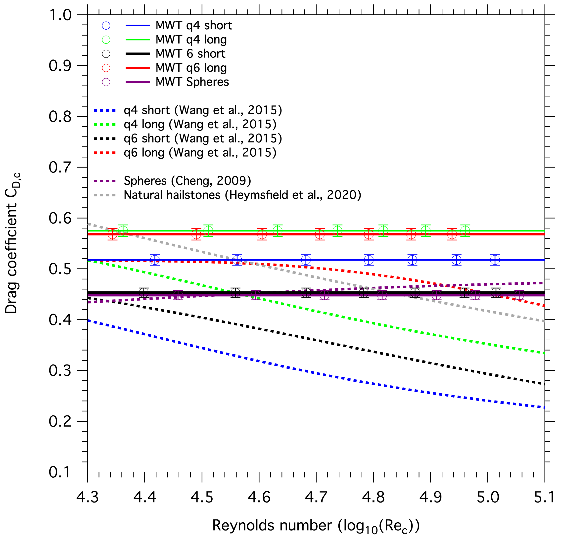
A necessary condition to apply this approach is the independence of $C_D$ from $Re$. As will be shown below in more detail the correction method extrapolates the data which are affected by the walls to free conditions, i.e., to a $BR$ of 0. Afterwards, that obtained value is used to correct the data along a certain Reynolds number range. Thus, to correct our data we had to verify that the drag coefficient is also constant in the observed Reynolds number range. This was done by printing four stones of each hailstone category and spheres, all with a maximum diameter of 3 $\mathrm{c}$$\mathrm{m}$ but with varying densities between $0.3$ $\mathrm{g}$ $\mathrm{c}$${\mathrm{m}}_{-3}$ and $4.2$ $\mathrm{g}$ $\mathrm{c}$${\mathrm{m}}_{-3}$. The lower densities were obtained by varying the infill of the print material and the higher ones by adding lead spheres into the center of the stones. We were restricted to the 3 cm size of the hailstones, because on one hand the stones should be as small as possible in order to reduce the blockage effect, and on the other hand, they should be large enough to equip them with lead spheres. The resulting $BR$ was about 7%.

Figure 4 shows the results of the data. The symbols and the lines are the data points and the average over the individual four data points. All four hailstone categories reveal a constant drag coefficient in a Reynolds number range from $Re\approx$ 20,000 to $Re\approx$ 85,000. The error bars indicate a measurement uncertainty of 6%. It was obtained by applying gaussian error propagation to Equations (1) to (4). The spheres have the lowest average drag coefficient of $C_D=0.50\pm 0.03$ and show no significant difference to the q6 short hailstones which have an average value of $C_D=0.53\pm 0.03$. The q4 short category possess an average value of $C_D=0.57\pm 0.03$ which is also within the error of the q6 short category. However, all the aforementioned categories have significantly lower values than the long lobed hailstones. The q4 long and q6 long categories show almost identical average values of $C_D=0.68\pm 0.04$ and $C_D=0.67\pm 0.04$. The results indicate that the number of lobes does not change the drag coefficient in the investigated Reynolds number range but the length of the lobes does. The short lobed categories seem to behave more like spheres, and therefore have similar drag coefficients. The important information of Figure 4 is that the drag coefficient is constant over a wide Reynolds number range. This fact allowed us to apply the semi-empirical wall constraint correction method of Awbi and Tan [22] which is described in detail in the following.

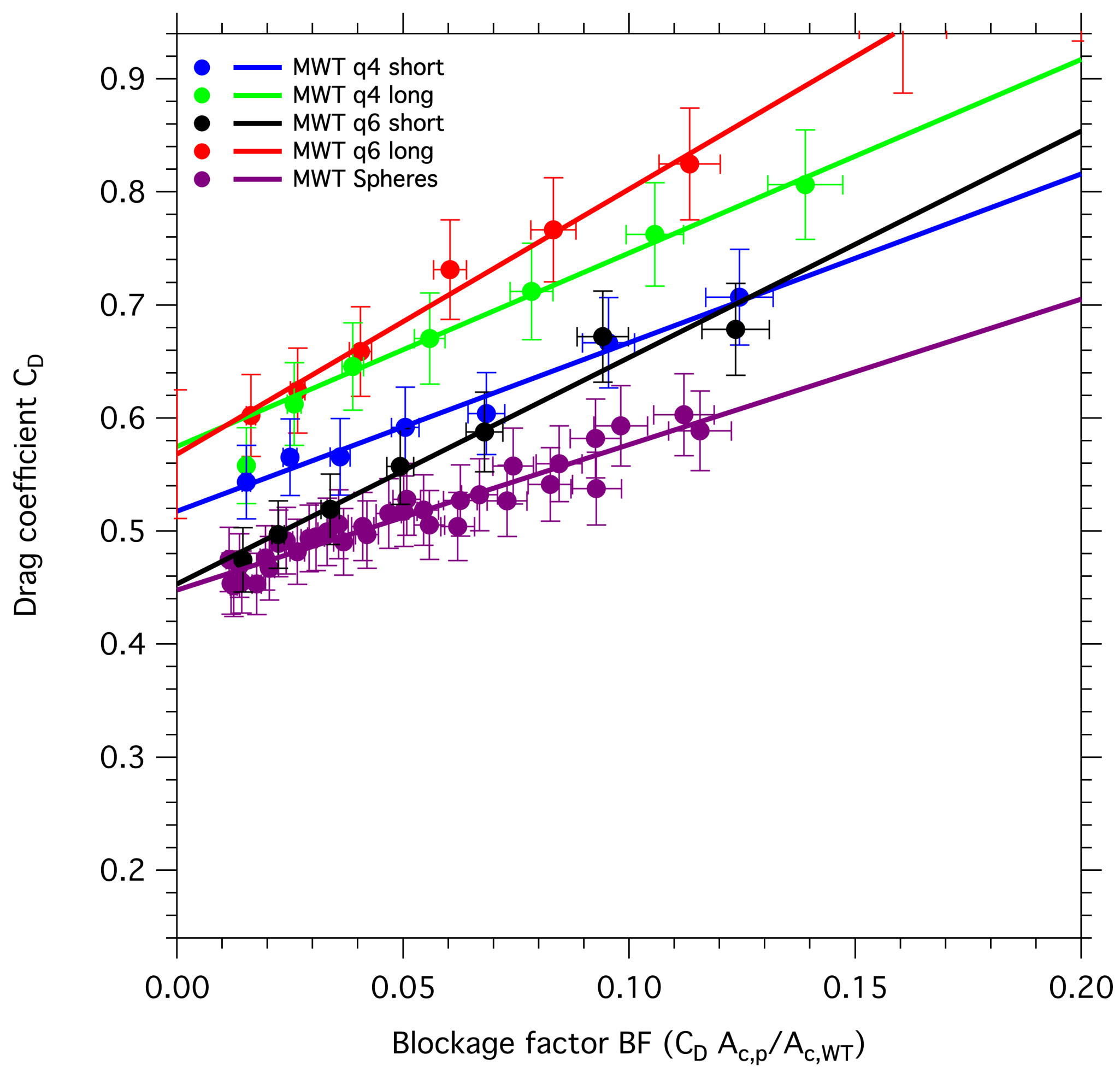
Figure 5 depicts the drag coefficient as obtained from the experiments described in Section 2.2 versus the blockage factor, i.e., $BF=C_D{A}_{c,p}/A_{c,WT}$. All data points show a linear trend against the blockage factor in the investigated Reynolds number range. From the extrapolations of the linear regressions to $BF=0$ the free drag coefficient is obtained and listed in

Table 4. Values of the extrapolated drag coefficients. The error is given by the $95.4$% confidence interval of the linear regression, which is about 2%.

Hailstone	${\mathit{C}}_{\mathit{D}}\pm \mathbf{\Delta }{\mathit{C}}_{\mathit{D}}$
spheres	$0.448\pm 0.010$
q4 short	$0.518\pm 0.014$
q4 long	$0.575\pm 0.012$
q6 short	$0.457\pm 0.008$
q6 long	$0.568\pm 0.016$

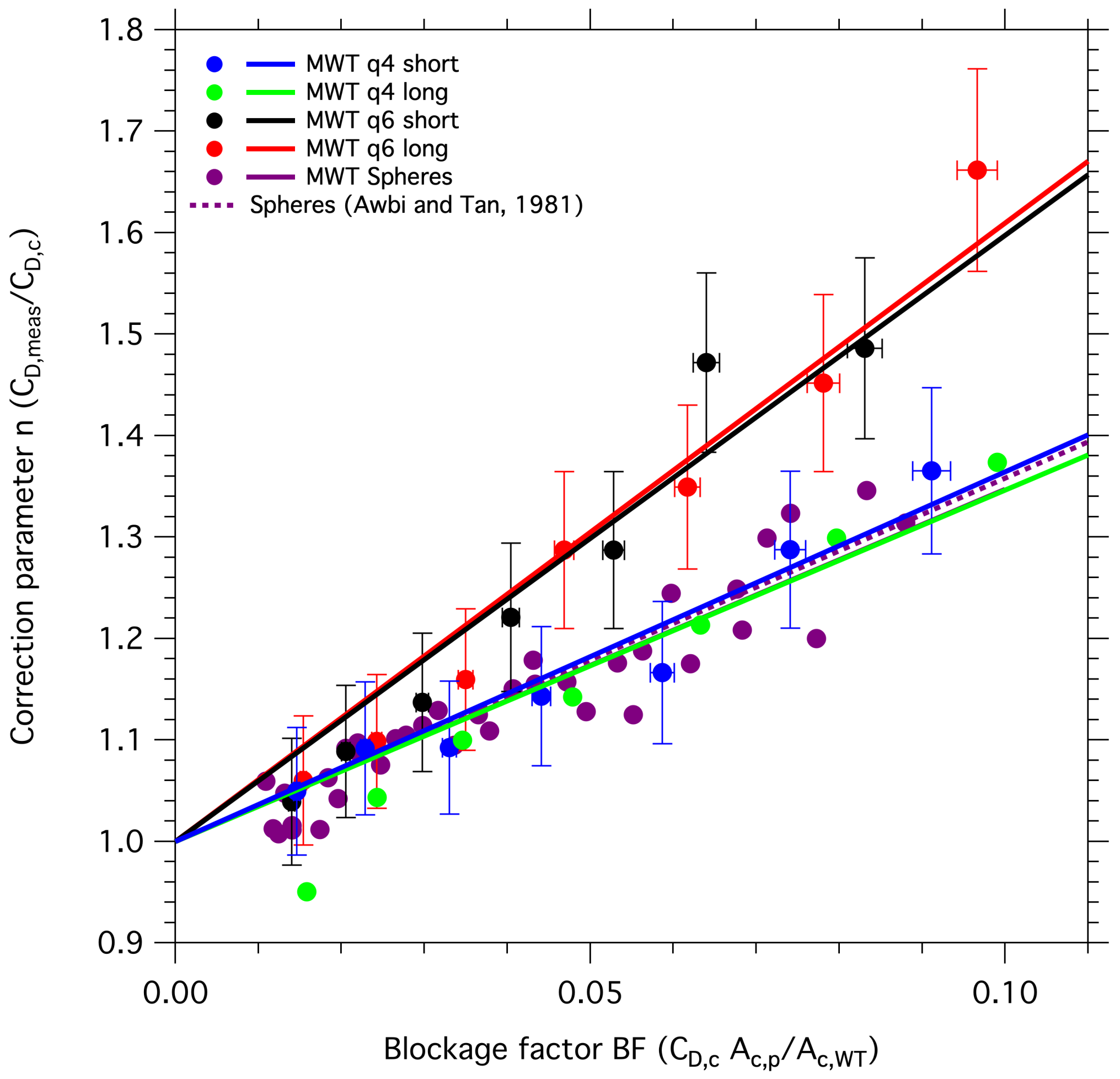
. Free in this context means no influence of the walls. From the extrapolated $C_{D,c}$ the blockage correction parameter n was calculated and plotted as function of $BF$ in Figure 6.

The correction parameter is definitely higher for the q6 hailstones than for the q4 hailstones and the spheres. This indicates that $C_D$ of the q6 categories is more affected by the walls than the other categories. That can be explained by the low pressure in the wake region which is decreased when the number of lobes is higher. Also shown in Figure 6 is a curve for spheres obtained by Awbi and Tan [22] (dashed purple line). The blockage coefficient $ϵ$ coincides remarkably good with the one derived in our study for the spheres, which is a verification of our measurement.

Table 5. Values of the blockage coefficients $ϵ$ (slopes of the curves in Figure 6). The error is given by the $95.4$% confidence interval of the linear regression.

Hailstone	$\mathit{ϵ}\pm \mathbf{\Delta }\mathit{ϵ}$
Spheres (Awbi and Tan, 1981)	3.58
Spheres	$3.47\pm 0.24$
q4 short	$3.64\pm 0.40$
q4 long	$3.46\pm 0.64$
q6 short	$5.97\pm 0.72$
q6 long	$6.09\pm 0.60$

shows the values of the blockage coefficient $ϵ$ which were derived from the slopes of the linear regressions as well as the value of Awbi and Tan [22].

3.2. Comparison of the Results with Literature

3.2.1. Drag Coefficients

Figure 7 shows the drag coefficient as function of the Reynolds number, both corrected for the blockage effect as described in Section 3.1, in comparison to literature values for the four hailstone categories as well as for spheres [12,24]. The extrapolated value of $C_{D,c}$ are summarized in Table 4.

Basically, the results reflect a similar trend as discussed for Figure 4. The spheres and the q6 hailstones are very close to each other and show the lowest values. However, while the averaged drag coefficient from Figure 4 show no significant difference between the q6 short and the q4 short category, the extrapolated results from Figure 5 do. A reason for that is that the influence of the walls on the drag coefficient varies between the hailstone categories as is obvious from the blockage correction coefficients given in Table 5. The q6 categories have larger epsilon values compared to the q4 categories and spheres. Thus, the distance in $C_D$ between categories q4 short and q6 short compared to Figure 4 when extrapolated from $BR=7\%$ to $BR=0\%$. The results for the spheres and the short lobed categories imply, that there must be a transition in $C_D$. Hence, when starting from a sphere and increasing the number of short lobes to a certain number (from 0 to 32) enhances the drag coefficient. However, by further increasing the number of lobes (from 32 to 72) the drag coefficient decreases again. But this effect can only be seen for the short lobed categories. The long lobed hailstones own the highest values of $C_D$ indicating that increasing the length of the lobes increases $C_D$. The transition in $C_D$ when increasing the number of lobes as in the short lobed categories vanishes for the long lobed hailstones resulting in almost identical drag coefficients.

The formulation of Cheng [24] for spheres suggests a slight increase in $C_D$ in the observed Reynolds number range. Due to the correction method applied in our analysis as well as the measurement uncertainty we cannot resolve such a behavior. Nevertheless, within the measurement error, our obtained $C_D$ value matches the curve of Cheng [24] quite well throughout the whole investigated $Re$ range. The comparison of our data and Wang et al. [12] reveals some deviations. The first difference is the dependency of $C_D$ on $Re$ found by Wang et al. [12], which was not reproduced in our wind tunnel measurements (see Figure 4). Furthermore, the drag coefficient increases for an increasing number of lobes in Wang et al. [12] which cannot be confirmed by the present results. In contrast to the findings of Wang et al. [12], the long lobed categories in the present study revealed no influence of the number of lobes on the drag coefficient. A comparison of the results of Wang et al. [12] for the q4 and q6 categories with our data at a mean Reynolds number of ${log}_{10}Re=4.7$ shows a decrease of 28% and 12% for the long lobed categories and 42% and 22% for the short lobed categories. In the short lobed category we observed a lower $C_D$ for the higher number of lobes which is contradictory to the results of Wang et al. [12]. The comparison indicates that for all four hailstone categories the experimentally derived drag coefficients are significantly higher than the numerically derived values obtained by Wang et al. [12]. Nevertheless, the trend that the long lobed categories have higher drag coefficients than the short lobed ones could be confirmed by our study.

There are several reasons for the deviations which make a direct comparison difficult. First, the drag coefficients in Wang et al. [12] were obtained at a pressure level of 900 $\mathrm{h}$$\mathrm{Pa}$. This might affect the drag coefficient compared to surface pressure conditions in our wind tunnel study because the drag is determined by the integral of the pressure distribution at the hailstone’s surface. Second, independently of the number and size of the lobes Wang et al. [12] approximated the terminal velocity with that of spheres with the same size, i.e., they overestimated the terminal velocity as shown below. Especially for the long lobed hailstones the terminal velocity deviates considerably from that of a sphere. This overestimation causes a shift in $C_D$ towards higher Reynolds numbers. Third, the orientation of the hailstones is different. Wang et al. [12] used a fixed orientation, i.e., the poles were parallel to the flow (see Figure 1). However, our experiments were performed by freely floating the particles. Thus, they could move arbitrary in the air stream. Even though their orientation changed as they were freely floating, we observed that they were preferentially oriented with the poles perpendicular to the flow, which very likely alters the flow field around them. Also, there might be some unknown effects from the simulations of Wang et al. [12]. An indication for that is given in Cheng and Wang [13]. The authors simulated the flow field of spherical hailstones at surface conditions. They found a steep drop in the drag coefficient of spherical hailstones starting at a Reynolds number of $Re={10}^{4.5}$. This drop is attributable to the critical transition regime from a laminar to a turbulent boundary layer. However, most experimental studies (e.g., Achenbach [25], Clift et al. [26]) show that the critical transition does not start before a Reynolds number of $Re={10}^{5.2}$. This is also supported by our results which show that the drag for spheres is constant until at least $Re={10}^{4.85}$ (see Figure 4). Conversely, the decreasing trend of $C_D$ with increasing $Re$ of the Wang et al. [12] data was also found for natural hailstones by Heymsfield et al. [27] which is indicated by the gray dashed curve in Figure 7.

3.2.2. Reynolds Number-Best Number

The Best number is of special importance as it can be calculated solely from physical parameters of the fluid and the particle. This makes it a suitable quantity to parameterize the Reynolds number [7]. Once these parameters are known the terminal velocity can be calculated from the $Re-X$ relationship, which can be considered as a generalization of the usual relationship of the terminal velocity on the maximum dimension as it accounts for the fluid density as well as for the mass and the cross-sectional area of the particle. That means, as long as the shape does not vary significantly, the terminal velocity can be calculated from the $Re-X$ relationship for different altitude levels and particle densities.

Figure 8 shows the corrected Reynolds number ($R{e}_c$) (see Section 3.1 and Equation (5)) versus the Best number (X) for the present results as well as for spherical and natural hailstones. The solid lines represent the wind tunnel data and the dashed lines are parameterizations from observations of natural hailstones and spherical hailstone models from the study of Heymsfield et al. [27] (gray dashed curve);

$$\begin{array}{ccc}\hfill Re& =& 0.41X^{0.56},\hfill \end{array}$$

(6)

and from Rasmussen and Heymsfield [28] (orange dashed curve);

$$\begin{array}{ccc}\hfill Re& =& {\left(\frac{X}{0.6}\right)}^{0.5}.\hfill \end{array}$$

(7)

Both parameterizations are valid within our observed Reynolds number range, i.e., $2\times {10}^4\le Re\le 1\times {10}^5$. A constant $C_D$ value, as obtained from the present results, leads to equal slopes of 0.5 in a $log-log$$Re-X$ plot. Thus, the Reynolds number can be easily determined from X by rearranging Equation (4) using the values given in Table 4. In contrast, a slope which differs from 0.5 means that the drag coefficient varies with Best number as is the case for natural hailstones (see the slope of the gray dashed line in Figure 8). That is, $C_D$ decreases with increasing size and mass (see also Figure 7). Nevertheless, the curve of Heymsfield et al. [27] is in good agreement with our data showing an average deviation of 10% for the arbitrarily chosen q4 long hailstone. The curve for spherical hailstones given in Rasmussen and Heymsfield [28] results in the lowest values of $Re$, which is due to the use of a constant drag coefficient of 0.6. Even though this value has been often used in literature for ice particles (e.g., Böhm [29]), it compares to the present results with a higher uncertainty than the parameterization of Heymsfield et al. [27]. The deviation from the curves of the present study and the parameterization of Rasmussen and Heymsfield [28] are 4% for the long lobed hailstones and 33% for the spheres which can be viewed as lower and upper limits.

3.2.3. Terminal velocity

Figure 9 depicts the corrected terminal velocity as function of the maximum dimension of the hailstones. Symbols and solid lines represent the present results, the dashed and dotted lines are parameterizations according Heymsfield et al. [27] (Equation (8));

$$\begin{array}{c}\hfill U=8.4D^{0.67},\end{array}$$

(8)

and Pruppacher and Klett [7] (Equation (9));

$$\begin{array}{c}\hfill U=0.36{\left(\frac{{\rho }_{H}D}{C_D{\rho }_a}\right)}^{0.5},\end{array}$$

(9)

where ${\rho }_H$ is the hailstone density (${\rho }_H=$ $0.91$ $\mathrm{g}$ ${\mathrm{m}}^{-3}$) and ${\rho }_a$ the density of dry air at 20 ${}^{\circ }\mathrm{C}$ (${\rho }_a\approx 1.2\mathrm{k}\mathrm{g} {\mathrm{m}}^{-3}$). The solid lines represent power law fits of the form:

$$U=a{D}^b$$

(10)

The values of the fit parameters a and b are summarized in

Table 6. Values of regression coefficients a and b when applying a power-law fit (see Equation (10)) to the $U-D$ data from Figure 9. The errors are given by the $95.4$% confidence intervals of the regressions.

Hailstone	$\mathit{a}\pm \mathbf{\Delta }\mathit{a}$	$\mathit{b}\pm \mathbf{\Delta }\mathit{b}$
Spheres	$14.84\pm 0.09$	$0.50\pm 0.01$
q4 short	$13.97\pm 0.26$	$0.50\pm 0.02$
q4 long	$12.44\pm 0.19$	$0.50\pm 0.02$
q6 short	$13.14\pm 0.37$	$0.55\pm 0.02$
q6 long	$11.87\pm 0.07$	$0.49\pm 0.01$

. Figure 9 reveals an apparent deviation of the terminal velocity of lobed hailstones from that of a sphere. This is especially pronounced for the long lobes hailstones. The spheres show the highest terminal velocities followed by the short lobed categories which both are within the errors of each other. This can be attributed to a compensation of the mass and the drag coefficient. The q6 short hailstones have almost the same drag coefficient as the spheres, however, they possess a lower mass compared to the q4 short hailstones (see Figure 2), which adapt both curves. The deviation for the short lobed category from spherical particles is 6% at $D=3.5\mathrm{c}\mathrm{m}$. The difference in the terminal velocity of the long lobed stones arise mainly due to the difference in mass, because the values of the drag coefficients $C_D$ are identical within the measurement error. The deviation of the terminal velocity from the spheres is 17 for the q4 long category and 21% for the q6 long category. This reduction needs to be accounted for in numerical simulations of lobed hailstones as it affects not only the flow field of the hailstones but also the convective-diffusive heat and mass transfer from or to a hailstone, and thus the ventilation effect. The parameterization of Pruppacher and Klett [7] is valid for roughly spherical hailstones and depends on the drag coefficient. Therefore, it is plotted for a literature value of the drag coefficient of $C_D=0.6$ and the one obtained here for spheres. It shows excellent agreement when our drag coefficient for spheres, i.e., $C_{D,c}=0.45$, is applied. However, when $C_D=0.6$ the terminal velocity is reduced by 14% or $3.7$ $\mathrm{m}$${\mathrm{s}}^{-1}$ compared to spheres at $D=3.5 \mathrm{c}\mathrm{m}$. The large deviation from the parameterization of natural hailstones from Heymsfield et al. [27] might be explained by the lower masses of natural hailstones. The aspect ratio decreases for increasing size of the hailstones (see e.g., Figure 5 in Heymsfield et al. [3]). Thus, even when the maximum dimension is the same as for a sphere the mass deviates considerably as can be seen from Figure 2.

3.2.4. Kinetic Energy

The above consideration for the terminal velocity shows that the parameterization for spheres overestimates the terminal velocity of about 6% when compared to short lobed hailstones. However, the kinetic energy ($KE$), which can be viewed as a measure for the destructive potential of hailstones, in this case would deviate considerably more due to the square in the velocity. Figure 10 shows the relationship of the kinetic energy, i.e., $KE=0.5m{U}^2$, and the maximum dimension. The values of the coefficients of the power-law fits are given in

Table 7. Values of regression coefficients a and b when applying a power-law fit ($a{D}^b$) to the $KE-D$ data from Figure 10. The errors are given by the $95.4$% confidence intervals of the regressions.

Hailstone	$\mathit{a}\pm \mathbf{\Delta }\mathit{a}$	$\mathit{b}\pm \mathbf{\Delta }\mathit{b}$
Spheres	$0.0565\pm 0.0074$	$3.96\pm 0.09$
q4 short	$0.0634\pm 0.0154$	$3.70\pm 0.16$
q4 long	$0.0374\pm 0.0078$	$3.76\pm 0.14$
q6 short	$0.0496\pm 0.0072$	$3.75\pm 0.09$
q6 long	$0.0366\pm 0.0085$	$3.54\pm 0.15$

. It illustrates that KE for the q4 and q6 short categories deviates from spheres at $D=3.5\mathrm{c}\mathrm{m}$ by 19% and 33%, respectively. For the q4 and q6 long categories the deviation from a sphere is 49% and 62%, respectively. The kinetic energy of natural hailstones, which is indicated by the gray dashed line in Figure 10, is reduced by 76%, which is due to the combination of the lower mass of natural hailstones and the associated lower terminal velocity. The deviation is even more pronounced for larger sizes, which highlights the importance of the correct representation of the crucial quantities such as mass and terminal velocity of hailstones in cloud models.

4. Summary and Conclusions

Wind tunnel experiments were performed to investigate the effect of lobes on the aerodynamic behavior of hailstones. For this purpose we used the mathematical equations given in Wang et al. [12] to generate 3D models of lobed hailstones with different surface properties, i.e., number and length of lobes. The q4 category has 32 lobes on the surface and the q6 72. For both categories a set with short and long lobes were investigated. Additionally, we tested spheres for comparison. The artificial hailstone models and the spheres were freely floated in a laminar airstream in the Mainz vertical wind tunnel to obtain their terminal velocity, fall mode, and thereof the drag coefficient.

Due to wall effects the wind tunnel data had to be corrected. Here we applied a semi-empirical correction method by Awbi and Tan [22] which matches our data for spheres remarkably well. The correction method indicated that the q6 category, i.e., the stones with the higher number of lobes, is more affected by the walls compared to the q4 category, with a lower number of lobes, and the spheres.

We found that the drag coefficients for all four lobed hailstone categories and spheres are independent of the Reynolds number in a range between ${10}^{4.4}\lesssim Re\lesssim {10}^{4.9}$. Spheres have the lowest drag coefficient of $C_D=0.45$. The stones with short lobes reveal a transition of the drag coefficient, i.e., $C_D$ of the q4 short category is 16% higher compared to spheres ($C_D=0.52$). However, increasing the number of lobes will reduce the drag coefficient again to $C_D=0.46$ for the q6 short case. This transition was not observed for the long lobed categories; both of them show equal drag coefficients of about $C_D=0.57$. The data of the present study for spheres show good agreement with literature. However, the results reveal some disagreement with the numerical simulations of Wang et al. [12] but likely this is mostly due to the differently chosen boundary conditions, i.e., pressure level, fall speeds, and orientation. We provide a Reynolds number versus Best number relationship which can be used to calculate terminal velocities of lobed hailstones for different sizes and densities. Although the drag coefficient for natural hailstones varies our data is in agreement with the $Re-X$ relationship derived by Heymsfield et al. [27], showing an average deviation from the q4 short category of 10%. The spheres were found to have the highest terminal velocities among objects having the same maximum dimensions. The terminal velocities of short lobed categories are on average reduced by 6% showing that they can be treated as quasi-spheres in cloud models without a strong deviation. However, the q4 long and q6 long categories deviate by 17% and 21%. This deviation needs definitely to be accounted for when numerically simulating the flow fields of lobed hailstones. The terminal velocity for spheres determined in our experiments can be described by the parameterization for roughly spherical hailstones given in Pruppacher and Klett [7], when the drag coefficient of $C_D=0.45$ is used. For reliably predict the kinetic energy of the hailstones at the ground it is crucial to correctly parameterize their mass and terminal velocity. The derived $KE-D$ relationship shows that the deviation from spheres is up to 70% for the largest investigated stones of 5 $\mathrm{c}$$\mathrm{m}$.

Finally, our study shows that surface properties do have a significant effect on the drag coefficient, and thus on the terminal velocity. Lobes on the surface of hailstones reduce the kinetic energy, and thus the destructive potential at the ground. Therefore, the results presented here contribute to our basic understanding of the influence of lobes on the microphysical properties of hailstones. The derived parameterizations can be used in cloud resolving models to improve the microphysical description of hailstones and thereby achieve a better prediction of the destructive potential of a hailstorm. In particular; given that the conditions within and below a cloud favor the growth of lobed hailstones (see Figure 1 in Wang et al. [12]) the destructive potential can be better estimated with the parameterizations provided here. Moreover, our results can be applied to future studies which numerically simulate the flow fields and the associated quantities such as the ventilation coefficient and the growth rate a of lobed hailstones. The present experiments were our first step in the investigation of the influence of lobes on the microphysics of hailstones. The next step will be the investigation of the influence of lobes on the ventilation effect and growth rates. Another key question arising from the present experiments is whether or not the hailstones tumble or gyrate in a natural setting, i.e., with no walls effects and at lower pressures. The authors of the present work plan a field study to investigate this question in the near future.