Article

Numerical Modeling for the Accidental Dispersion of Hazardous Air Pollutants in the Urban Metropolitan Area

School of Urban and Environmental Engineering, Ulsan National Institute of Science and Technology (UNIST), Ulsan 44919, Korea
*
Author to whom correspondence should be addressed.
Atmosphere 2020, 11(5), 477; https://doi.org/10.3390/atmos11050477
Submission received: 24 March 2020 / Revised: 1 May 2020 / Accepted: 4 May 2020 / Published: 8 May 2020
(This article belongs to the Special Issue Recent Advances of Air Pollution Studies in South Korea)

Abstract

:
A numerical simulation system is developed to predict the dispersion of hazardous air pollutants (HAPs) over a populated city due to accidental release. Ulsan, as one of the megacities in Korea, is chosen as an ideal testbed for the simulation, as it is located in complex terrain and hosts a national industrial complex on the outskirts of the city. The system is based on the California puff model (CALPUFF) for simulating a HAP’s dispersion, in which the three-dimensional atmospheric circulation derived from the observed weather station data is specified at a fine horizontal resolution of 200 m. A test scenario is developed for the accidental release of benzene during the daytime and nighttime, respectively, by a fictitious explosion of a storage container, and the injection amount is determined arbitrarily yet comparable to those in the past accidents. In attempting a quantitative assessment and zoning the level of potential risk over the impacted area, multiple simulations have been conducted each day with different hourly varying meteorological conditions in August. The dispersion characteristics of the air pollutant depend largely on the local wind patterns that vary substantially from day to day. Nevertheless, the composite analysis sufficiently identifies the impacted area by the HAP’s dispersion due to the local prevailing wind such as the land–sea breeze circulation. An immediate hazardous area is determined based on the vulnerability map constructed by zoning the level of risk determined by the spatial distribution of the HAPs’ concentration and the harmfulness standard to the human body.

1. Introduction

Modern industry uses various kinds of chemicals, which can be not only the source of air pollutants gradually degrading ambient air quality but also often cause hazardous accidents. The dense populations in urban cities tend to increase vulnerability, even with narrow pollutant dispersion from nearby accidents [1]. There were several notorious accidents, including the case in Bhopal, India, in 1984, which resulted in more than 200,000 casualty losses. Another was the natural gas leak in Porter Ranch, California, in 2015–2016, which continued over four months and led to the relocation of up to 5000 residents.
In South Korea, about 42 accidents occur on average per year based on the national statistics reported by the Korea Research Institute of Chemical Technology for 2003–2018 [2]. The accident that happened in Gumi in 2012 was the worst, where the hydrogen fluoride (HF) gas leaked from a chemical-producing factory, causing 23 casualty losses. The devastating effects included killing crops and livestock in the surrounding area and spread into the nearby river, causing water contamination. Although routine safety checks would reduce the chance of accidents, once the accident already happens, a rapid response system is needed to support the fast decision making and mitigate the casualty losses and property damages.
A rapid response can be made based on the information from the operational real-time monitoring network such as the one by the United States National Oceanic and Atmosphere Administration (NOAA) and the Environmental Protection Agency (EPA) [3]. However, it requires a dense monitoring network with many instrumental sensors to measure various types of chemicals and air pollutants. Although there exists a monitoring network operated by the Korean government for 31 species of HAPs, it is not sufficient in spatial coverage and only two stations cover the city of Ulsan, with a size of 1057 km2.
Another approach is to develop a response system based on reliable numerical dispersion models. For example, Taiwan developed an expert system for air pollution emergency response [4] by combining meteorological, air quality, and economic models. Further, NOAA and EPA provide the acute dispersion models and regulations such as the Areal Locations of Hazardous Atmospheres (ALOHA) model for predicting the spread of the pollutants [5] and the acute exposure guideline levels [6]. The geographic information system (GIS) is also combined with the numerical dispersion models in developing the emergency response system [7]. Compared with the monitoring-based approach, this model-based approach seems to be practically more useful in deriving potentially hazardous areas affected by an accident.
Atmospheric dispersion and exposure simulations have been researched by many previous studies applied to the various gases and aerosols. For example, [8] conducted numerical experiments for the simulation of the annual mean particulate matter (PM) concentration over Central America for 1999–2000. Other studies targeted for various cases such as the dispersion of sulfur dioxides [9,10,11], sulfides and nitrides [12,13], odor dispersions [14,15], metals and dissolved ions from incinerators [16], traffic pollutants [17], total suspended particulate matters (TSP) in quarries [18], and volcanic plume [19]. Derived time mean exposures of pollutants by numerical dispersion and transport models were further used to assess the health risk quantitatively based on prevailing wind and other meteorological conditions, average exposure concentrations, and the intake fraction by a human. The risk information was eventually displayed in space to show which areas were hazardous and which were not.
One of the limitations in the previous studies was in using limited cases of meteorological conditions. Meteorological conditions vary in time from sub-daily to daily, and from season to season, which can change the HAPs’ concentrations substantially in time and space. Therefore, the general evaluation of the risk of the accidental release of HAPs should be made by counting on changes in weather conditions over a sufficiently long period. This study develops a response system for Ulsan as one of the megacities in Korea, in which more than four heavy industrial complexes are located near the residential area within a few tens of kilometers. An investigation of the generalized dispersion patterns of HAPs over the target area identifies the most vulnerable places at the accidental release.
In Section 2, the used models, data, and experimental setup are described. Section 3 shows the modeling results and the analysis of the general risk of accidents. Section 4 is the highlights of the key results and overall discussions. A summary and concluding remarks are given in Section 4.

2. Experiments

2.1. Atmospheric Dispersion Model

The model used in this study is the California puff model (CALPUFF) [20], which has been used widely for solving various atmospheric dispersion problems in previous studies (e.g., [9,21,22]). In [23], showed that the model was able to simulate the dispersion of H2S differently according to the different meteorological conditions specified for flat land, land–sea, and mountain–valley geographies, and [24] modified the model to reflect the impacts of heterogeneous land surface conditions on the dispersion and local concentration of air pollutants. The models are based on the non-steady-state Gaussian puff model, which represents a dispersed plume consisting of several puffs (or lumps) of pollutants. Each puff is transported by the specified three-dimensional wind fields, and the size of the puff changes over time by the internal diffusion process with a Gaussian distribution. The concentration equations are formulated by [25] as below:
C = Q 2 π σ x σ y g   exp [ d a 2 2 σ x 2 ] exp [ d c 2 2 σ y 2 ]
where C is the ground-level concentration, Q is the pollutant mass in the puff, σx and σy are the standard deviations of the Gaussian distribution in the along-, cross-, and vertical-wind directions, respectively, and da and dc are the distances from the puff center to the receptor in the along- and cross-wind directions. In Equation (1), g determines the vertical dispersion as
g = 2 2 π σ z n = exp [ ( H e + 2 h ) 2 2 σ z 2 ]
where σz is the standard deviation of the vertical Gaussian distribution, He is the effective height above the ground off the puff center, and h is the mixed layer height.
The three-dimensional wind fields are derived from the discrete meteorological data through statistical interpolation and extrapolation from the California Meteorological Model (CALMET), which is a diagnostic model for processing meteorological data required for CALPUFF. CALMET is available for processing various meteorological data from observation stations or model simulation outputs to the gridded three-dimensional data. More detailed information is provided in the user’s guide for CALMET [26] and CALPUFF [25], respectively.

2.2. Experiment Settings

This study selects benzene as a representative chemical among the HAPs, which is the first-class carcinogenic chemical broadly used in our local study area. Benzene is a stable and non-polar chemical with low reactivity. The biggest reaction is the substitution of hydrogen, but it requires catalysts and a sufficient amount of heat. Therefore, this study disregards a secondary chemical reaction process under the normal outdoor atmospheric conditions and treats it as a pure dispersive gas by meteorological conditions. Table 1 shows the chemical properties of benzene specified in this study, following the Korean Ministry of Environment [27].
Figure 1 shows the modeling domain, in which the urban area with the industrial complex is surrounded by high mountain ranges and ocean. The surface elevation and the land cover type were specified based on the ASTER global digital elevation model version 2 (ASTGTM2) and Global Land Cover Characterization (GLCC), respectively. To produce the meteorological fields, CALMET processed the surface data from the local Automated Surface Observing System (ASOS) and unmanned automated weather stations (AWS), and the rawinsonde data in Pohang, which is the nearest available upper-level observation site.
The source point in the study domain was chosen as one of the industrial businesses located at 35.504 N, 129.353 E. This region is identified as the largest benzene emission area within the industrial complex, based on the annual emission and waste amount total reported officially to the government. Although the worst scenario of an accident is the entire leakage of all contained gas in the storage, this information is unavailable in public in Korea. The potential storage amount was estimated based on the waste transport, emission, and the displacement for each business industry reported to the government database of the Pollutant Release and Transfer Register (PRTR) [28]. Based on the record, the total waste of benzene transported in Ulsan in 2013 was 416,204 kg. The annual emission of benzene from the targeted point source was also recorded as 26,097 kg yr−1, which accounts for 39% of the total emission of 66,908 kg yr−1 in Ulsan. It is assumed that the waste amount is also proportional to the emission amount and this study applied 39% of the 416,204 kg yr−1 total in Ulsan, which is 162,319.56 kg yr−1 or 13,526.63 kg mon−1. Given the monthly waste total, this study further assumes that the storage will be replenished once for a month, then this amount of waste can be assumed as the amount of monthly storage. Our scenario is 60% leakage of the monthly storage to the atmosphere within 12 h, which is estimated at 94 g s−1, or 339 kg h−1. For comparison, Table 2 shows the record of past accidents that occurred in Ulsan based on the Integrated Chemical Information System (ICIS) [29]. In Table 2, the emission rate is simply estimated based on the duration period and total amount of leakages from the information system, which shows lots of variation. By comparing these with the emission scenario in this study, the value of 339 kg h−1 is the one likely to occur.
The minimum detection range of benzene in the air is known as 0.64 μg m−3 [30]. The annual standard for benzene in Korea is 5 μg m−3, and the US EPA defines the dangerous level of inhalation is 30 μg m−3 or higher according to the Integrated Risk Information System (IRIS) [31] and the Chemical Summary Report of the benzene [32] These values are used in the health risk assessment in Section 3.3.
The numerical experiments were conducted for the domain for 1–31 August 2013 at a 200 m spatial resolution. The reason for choosing August was to consider the effect of the spread of HAPs due to the regional circulation specific to Ulsan. The temperature of Ulsan is highest this month during the year and the local daytime sea breeze wind develops at its peak phase. Therefore, the dispersion to the adjacent residential area is more likely to occur in summer. Although this study focuses on summer, it is noted that the modeling framework developed in this study can be generalized easily to other seasons such as winter. Although not shown here, much stronger northwesterly winds prevail in winter, which tends to slow down the sea breeze and weaken the transport of atmospheric pollutants toward the inland region. The experiments were carried out twice a day. Each experiment was run for 12 h, started from the identical time of the day at 14:00 local standard time (LST), with an identical emission scenario of benzene. Therefore, the experiments have 31 simulation outputs, all of which have different chemical distributions in time and space due to the difference in meteorological conditions only. Hourly outputs were then averaged for a month for each hour of the day to depict the time-averaged dispersion characteristics driven by the local observed meteorological conditions. Chaotic weather variability was averaged out and the diurnal change in local circulation driven by the land–sea contrast became evident.

3. Results

3.1. Validations for Wind and the Test Cases

This study first validates the simulation of local wind by CALMET against the observations. Figure 2 compares the local wind variation, which is averaged each hour over August 2013. The observed local wind is westerly at noon and it turns into southeasterly at around 15:00 LST and to southerly until 20:00 LST, due to the development of the sea breeze in the study domain. By the weakening of the sea breeze and developing land breeze, the wind changes to northwesterly after 21:00 LST until 11:00 LST. In general, the observed and the simulated wind vectors are in good agreement in terms of direction and magnitude, which demonstrates that CALMET can represent the local observed wind variation realistically. When the daily mean wind components are removed and only the diurnal components are compared, the simulations also exhibit good agreement with the observations, although the overall magnitude is weaker than the observed. The CALMET diagnostic model adjusts the sparse wind observations onto the model grids at 200 m resolution, not only based on statistical interpolation using an inverse-distance method but also by considering the kinematic effects of the terrain, slope flows, blocking effects, and three-dimensional divergence minimization [22]. Therefore, the simulated wind is not exactly the same as the observed, although the difference is negligible. Note that the southerlies are relatively stronger than the northerlies, suggesting that the sea breeze is more pronounced than the land breeze in this region. August is characterized by strong diurnal wind variation in this coastal region, typically in summer. During winter, the observed winds are mostly northerlies with much suppressed diurnal wind variation (not shown).
Figure 3 compares the sample cases of benzene dispersion in time during the daytime and the nighttime accidents. These cases are chosen as the typical cases in the summertime weather in Ulsan, characterized by the local land–sea breeze circulation. The chemical dispersion pattern depends largely on the specified wind condition. The initial direction of the plume and the level of surface concentration is quite different between the daytime emission-started and the nighttime emission-started cases. When the emission starts in the afternoon at 14:00 LST, the emission plume tends to spread to the northwest by the developing sea breeze in the one hour after. It tends to move further northwestward by the enhanced sea breeze in the three hours after. The plume also becomes wider in the cross-wind direction by the diffusive nature of Gaussian puffs. Six h later at 20:00 LST, the sea breeze slows down and the overall wind becomes calm. The surface concentration shows a circular pattern with a slight stretch in the zonal direction by background winds. At 12 h after at 02:00 LST, the wind becomes northerly, suggesting the development of the land breeze in the nighttime, and the plume is advected toward the ocean. The surface concentration in the downstream tends to increase a lot by the nighttime suppression of the atmospheric boundary layer. Compared with the southerly sea breeze, the land breeze is much weaker and this is consistent with the results shown in Figure 2.
In the nighttime emission-started case, the initial plume moves eastward by weak background westerlies in the one hour after. The concentration tends to increase further in the downstream in the three hours after, with a more stretched plume in the along- and cross-wind directions. Six h later at 08:00 LST, the surface concentration tends to decrease, presumably due to the dilution by the development of the atmospheric boundary layer in the morning. The plume changes drastically in direction and it moves to the northwest by the strong sea breeze circulation in the afternoon at 14:00 LST, in the 12 h after emission.
Overall, CALMET represents the wind reversal by the local land–sea breeze circulation. Accordingly, the chemical dispersion pattern is realistic, reflecting the important role of local wind patterns.
This study further examines the mechanisms for a much higher benzene concentration in the nighttime compared with that in the daytime. Figure 4 shows the vertical cross-section of the benzene dispersion at the source point. The horizontal axis is aligned following the surface wind direction at the source point, whose direction is indicated separately for the daytime and the nighttime emission-started cases in Figure 1. As shown in Figure 3, the southeasterly sea breeze wind near the emission source transports the chemical to the northwest in the daytime emission-started case in Figure 4a. The dispersion pattern also shows a vertical expansion, thereby contributing to decreasing the concentration level near the surface. Note that the mixing height in the boundary layer for the daytime and nighttime is significantly different. Considering that the typical height of the atmospheric boundary layer is about 1–2 km [33], benzene tends to spread in the vertical direction due to the development of the atmospheric boundary layer during the daytime. In the meantime, surface heating during the daytime tends to induce a vertical upward motion, thereby driving a more enhanced vertical transport of the chemicals. The vertical motion is more accelerated at the increase in height due to less turbulence momentum mixing. On the other hand, strong subsidence develops on the opposite side, which is southeast to the emission source and toward the ocean. The wind pattern in Figure 4a shows the local sea breeze circulation developed in the daytime, with an upward motion over the land and downward motion over the ocean. It shows the sea breeze at the lower levels up to a few hundred meters, although there is uncertainty in the simulation for the vertical depth of the sea breeze circulation.
The dispersion pattern in the nighttime is quite contrasting to the case in the daytime. Due to the westerlies near the emission source in the nighttime, as shown in Figure 3, benzene spreads to the east in the figure. The surface cooling and nocturnal stable boundary layer tend to suppress the vertical dispersion of benzene. Further, the vertical motion in the lower atmosphere maintains weak subsidence, which tends to further inhibit the vertical transport of benzene. As a result, the dispersion sticks to the ground and the benzene concentration tends to be larger near the ground-level in the nighttime compared with that in the daytime. This explains why the impacted area by the high level of the benzene concentration becomes larger in the nighttime, as shown in Figure 3.

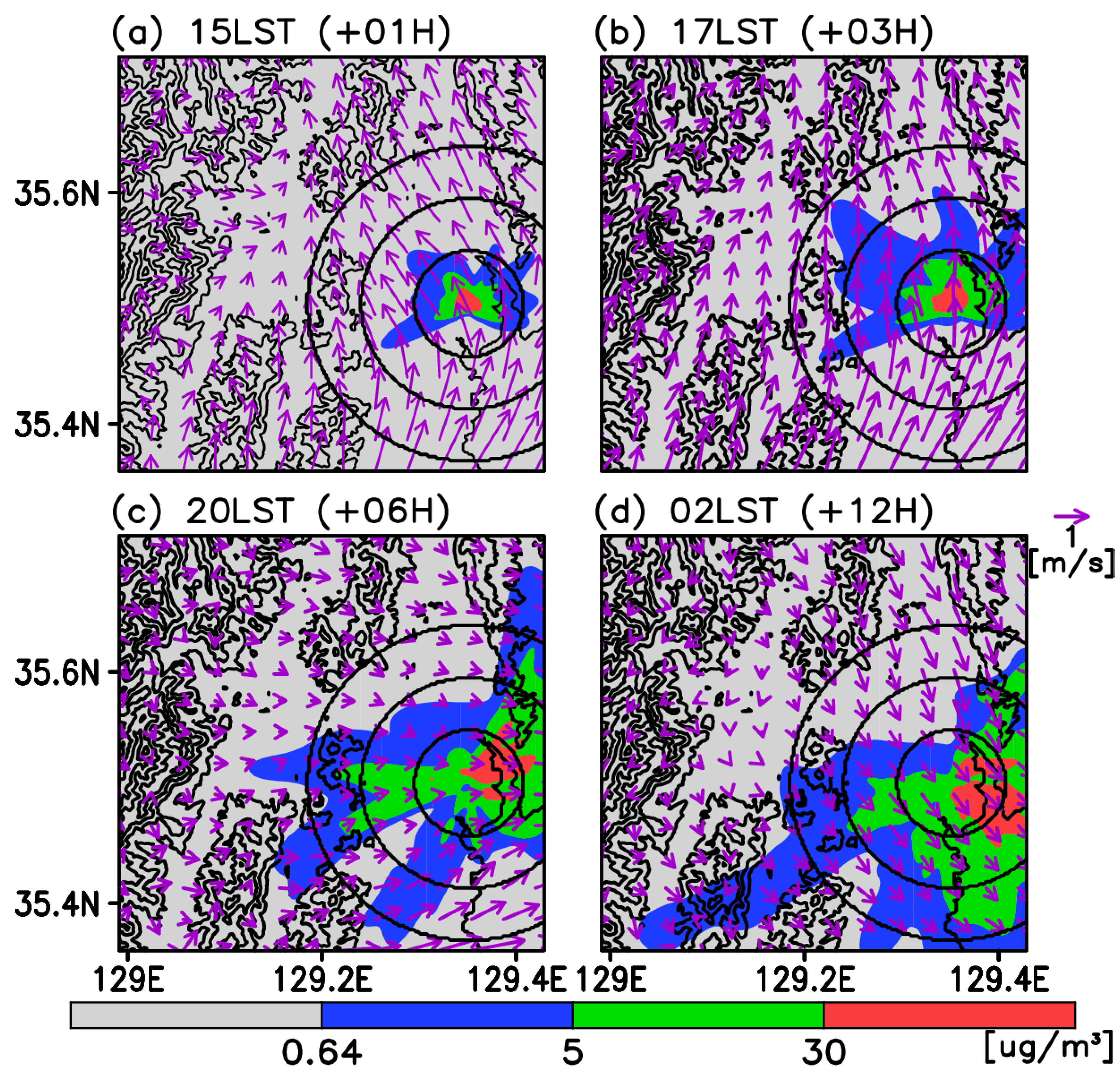
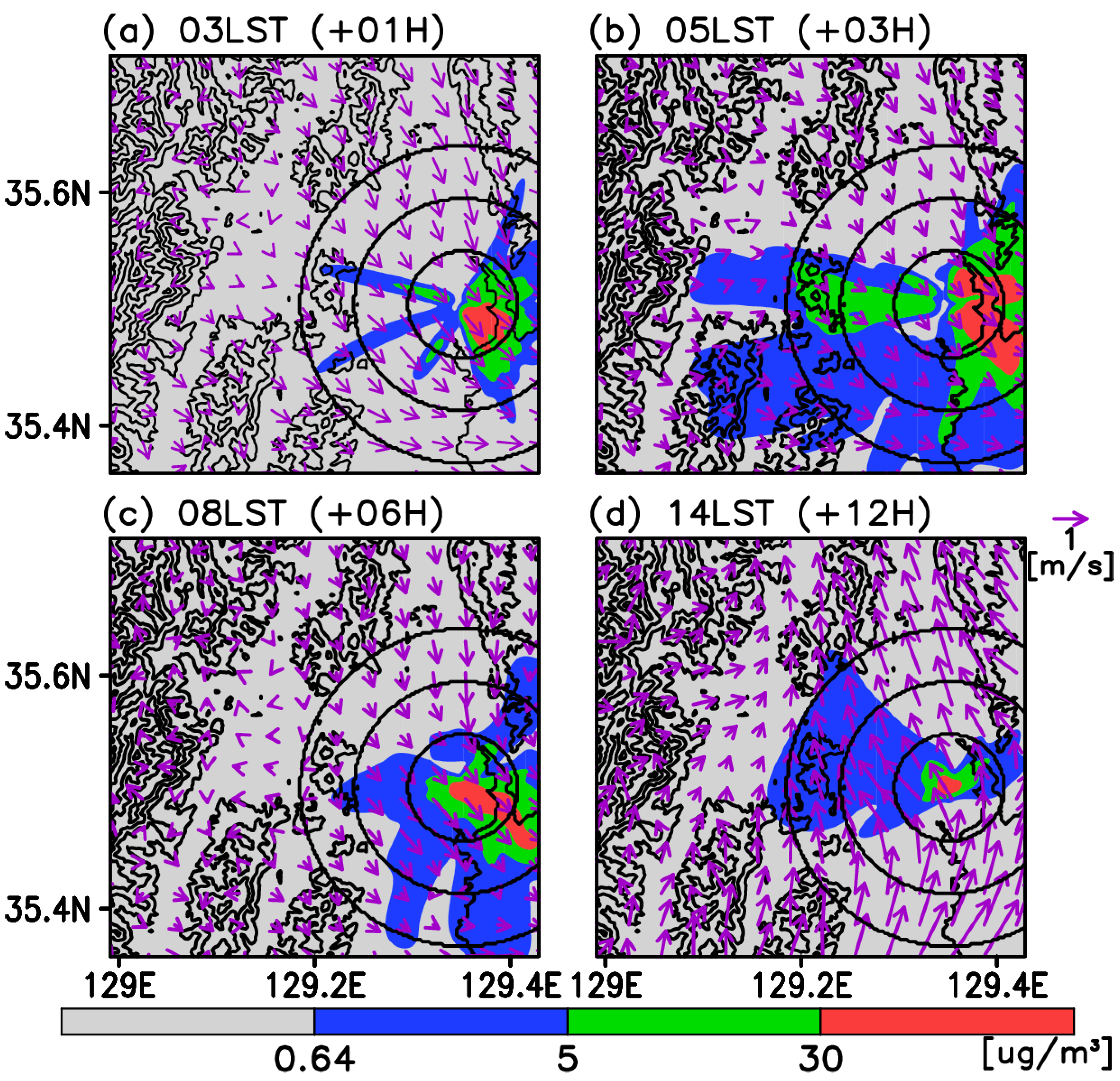
3.2. Time-Averaged Dispersion Pattern

The time-averaged dispersion patterns obtained from the numerical experiments for the entire 31 days in August represent the time evolution of the vulnerable area at the chemical accident in the summertime. For the daytime emission-started case (Figure 5), the wind variation shows much resemblance to that in the sample case of 15 April (Figure 3), and it shows the signal of the land–sea breeze circulation driven by the differential heating between the land and the ocean in the diurnal timescale more clearly by eliminating random weather variability. The sea breeze develops from the south during the afternoon to the early evening and the off-shore wind develops in the nighttime from the west in the late evening and from the north after midnight. The model also represents the impact of surface friction exerted on the wind realistically by slowing down the wind speed over the elevated mountain area.
Figure 5 also shows the time evolution of the time-averaged benzene concentration during the daytime emission-started cases. Each figure uses the color scheme with just three concentration levels of 0.64, 5, and 30 μg m−3, which are the minimum value of detection by the instrument, the annual standard of benzene concentration in Korea, and the dangerous level defined by US EPA, respectively. The averaged dispersion patterns show the hint of a few rapid dispersion cases affected by strong wind in specific dates, indicating that the one-month average is not sufficient enough to obtain generalized dispersion patterns. Nevertheless, the time evolution of the dispersion patterns still captures the basic features affected by the diurnal variation of the local circulation, particularly reflected in the higher concentration levels. Benzene dispersion shows a gradual expansion in the area over time of the continuous emission at the source point that started in the afternoon. Moreover, when the southerly winds prevail in the afternoon, benzene spreads to the north following the sea breeze. Then, it spreads southeastward by the weak land breeze from the late evening to the nighttime. Based on the simulations, the detectable range of benzene can be observed at the 5 km distance from the emission source in 1 h, 10 km in 3 h, and 15 km in 6 h. The benzene concentration level exceeds the annual standard value in Korea at the 5 km distance in 3 h and 10 km in 6 h, and 15 km in 12 h. The area under the dangerous benzene level stays within a 2 km radius from the emission source until 3 h after the emission. However, the area of dangerous level spreads quickly in the late evening and after midnight, reaching the 5 km distance after 6 h.
The wind variation during the nighttime emission-started cases (Figure 6) also shows much resemblance to the sample case of 16 August (Figure 3). The land breeze develops in the nighttime until it changes to a sea breeze in the afternoon. According to this, benzene tends to spread southeastward until the morning, and then northwestward in the early afternoon. Compared with the daytime emission-started cases, benzene tends to spread more quickly in the initial few hours in the nighttime emission-started cases. The detectable range of benzene can be observed mostly within the radius of the 10 km region from the source in one hour, and even at the 15 km distance it is affected in a few cases. In three hours, it is detectable beyond the 10 km radius in most of the downstream region. The spreading region becomes narrow in direction and more oriented toward the ocean, reaching out to the 15 km radius in 6 h (08:00 LST), as the land breeze develops more strongly at this time near the source point. When the sea breeze develops after 12 h (14:00 LST), benzene is not detectable in the southeastern area and it is carried to the land area and is detectable beyond the 15 km radius. The benzene concentration exceeds the annual standard and even reaches the dangerous level at the 5 km distance immediately within one hour after the emission. The dangerous area expands further and gets close to the 10 km radius in the downstream in 3 h. Compared with the case at 05:00 LST, the areas exceeding the annual standard and the dangerous levels tend to reduce within 6 h (08:00 LST), and this seems to be related to the dilution of benzene in the atmospheric boundary layer in the morning. Both the areas exceeding the annual standard and the dangerous level are confined within the 5 km radius within 12 h after the emission (14:00 LST).
The comparison between the daytime and the nighttime emission-started cases suggests that the dispersion can be more dangerous in the nighttime cases, especially for the initial few hours. This can be explained by the difference in the three-dimensional wind patterns. The air pollutant spreads more quickly and reaches further in the nighttime (c.f., Figure 5b and Figure 6b). Note that the near-surface wind is stronger in the daytime due to the development of the sea breeze, which would otherwise transport the pollutant further from the emission source than in the nighttime. However, a strong vertical motion (Figure 4a) tends to increase the vertical transport of the pollutant and therefore decreases the near-ground-level concentration in the daytime. The daytime heating over the land can induce a vertical motion. In addition, the sea breeze tends to decelerate as it penetrates through the land, and this induces horizontal convergence and a vertical motion. The daytime heating and the development of the atmospheric boundary layer also contribute to the vertical dilution of the air pollutant. On the other hand, the upward motion is quite suppressed in the nighttime. Further, the stable atmospheric boundary layer reduces the vertical dilution and it tends to increase in the near-ground-level concentration. During the nighttime, the overall wind magnitude is weak and the land breeze is not as pronounced as the sea breeze in the daytime. This also makes the prediction of the dispersion direction difficult. There are a few cases when the dispersion direction is opposite to the prevailing wind direction, such as the case shown in Figure 6a, and this indicates that the nocturnal wind variation is not as regular as that in the daytime.

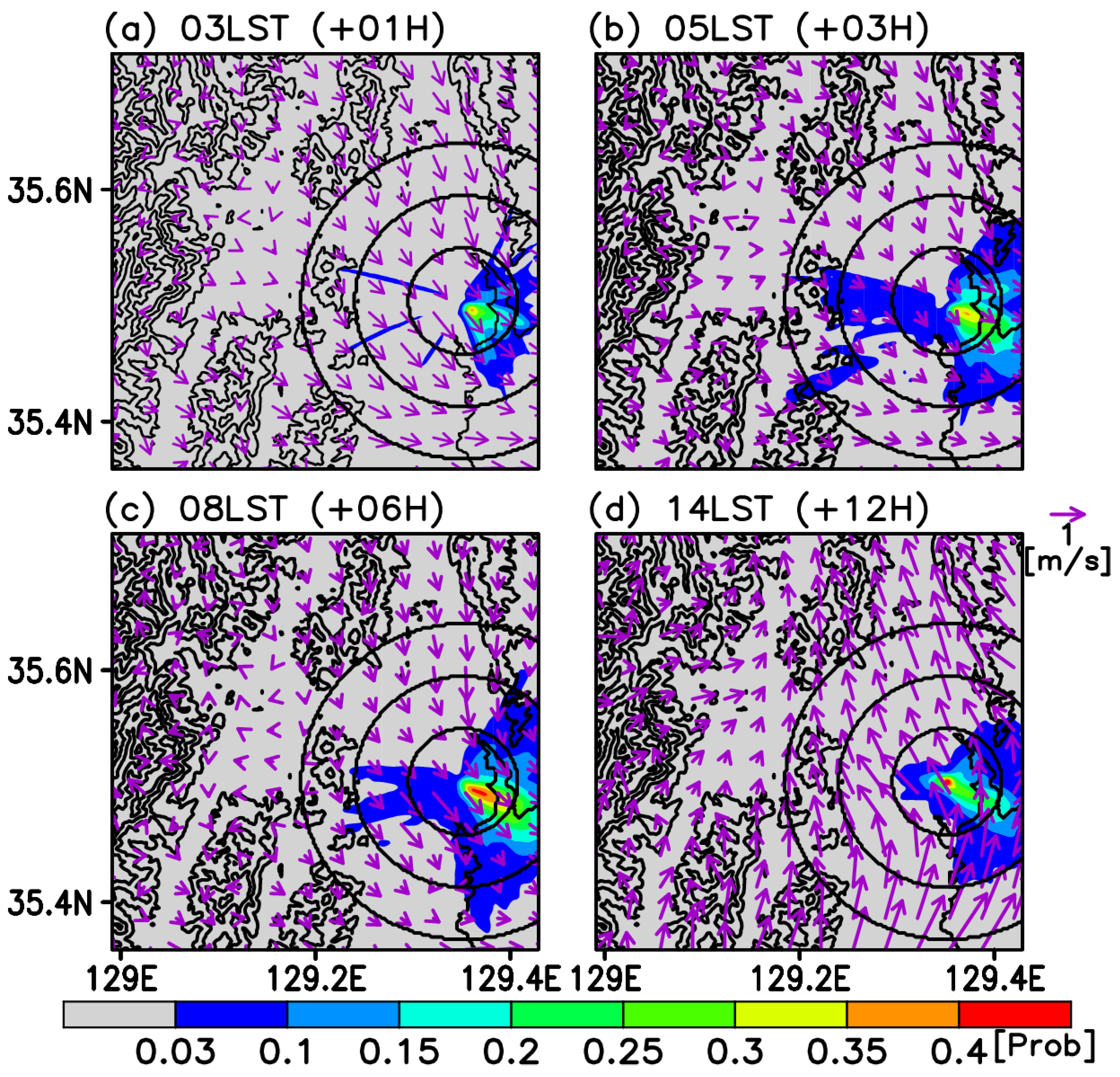
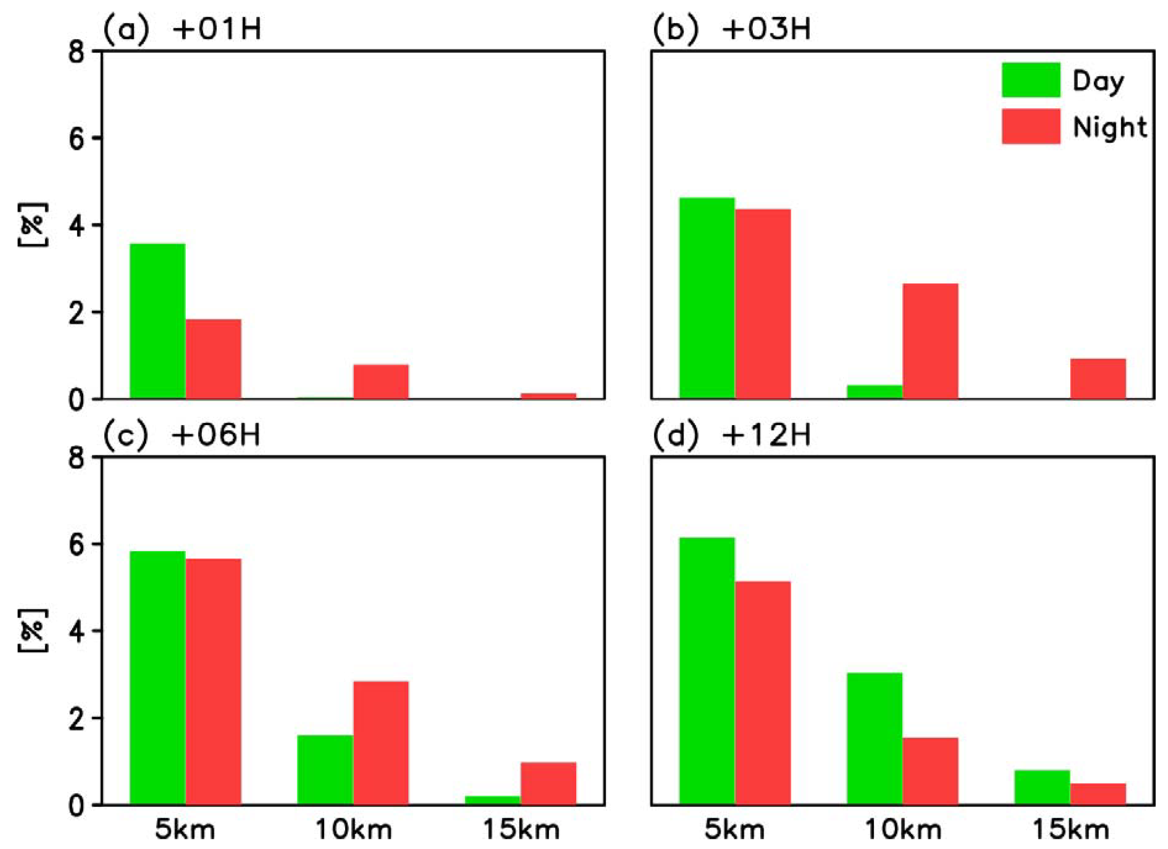
3.3. Risk Assessment

Previous time-averaged concentration patterns do not necessarily represent the vulnerable area by the chemical accident. When the wind is changing drastically during the accident, the time-averaged concentration tends to be low for the specific location, although that spot may be temporarily exposed to the dangerous level of 30 μg m−3 in the concentration. In this regard, the accumulated hit rate for each benzene concentration exceeds the dangerous level from the initial time to the designated hour and is examined for the daytime emission-started cases and the nighttime cases, whose results are shown in Figure 7 and Figure 8, respectively.
Overall, these accumulated hit rate patterns show more smoothed patterns in space when compared with their counterparts of the time-averaged patterns (i.e., Figure 5 and Figure 6). During the daytime emission-started cases (Figure 7), the vulnerable area tends to expand with time. In one hour, the hit rate near the 5 km radius from the emission source is less than 3%, and then it becomes 3% in the downstream region. In 6 h, the hit rate reaches as high as 10% at the 5 km radius, particularly in the downstream side. In 12 h, the hit rate tends to increase by more than 15% for those regions. In the meantime, the results indicate that the risk area more than 3% of the hit rate is mostly within the radius of 10 km from the emission source. Assuming that 3% is the threshold for taking action such as the enforcement of the evacuation of residents, the area within the 10 km radius from the industrial complexes should be carefully monitored for an immediate response to a chemical accident that may occur in the daytime.
Throughout the nighttime emission-started cases (Figure 8), the hit rate tends to increase in the downstream side, following the land breeze until the morning. The most contrasting feature to the daytime cases is the rapid increase of the hit rate for the initial 3 h. The hit rate becomes as high as 20% near the 5 km radius from the source in one hour, and then 20–30% in 6 h. In 12 h, the hit rate tends to increase more than 35% in the downstream side at the 5 km distance. In 12 h, the circulation is reversed and the hit rates tend to be steady or slightly decrease in the windward side. The result suggests that the risk area with more than 3% of the hit rate can expand up to the 15 km radius within 6 h after the accident. Therefore, a broader region should be monitored for an accident that may occur in the nighttime.
The risk assessment based on the accumulated hit rate in the above highlights that the vulnerable area expands more quickly in the nighttime emission-started cases in the downstream side, thereby increasing the potential health risk in the affected region. To examine this difference in a quantitative way, this study compares the accumulated hit rate averaged over land within the 5, 10, and 15 km radius from the emission source (Figure 9). In one hour, most of the exposures are concentrated within the 5 km radius after the daytime emission starts. The exposures over the area within the 5 km radius are less frequent in the nighttime emission-started cases, with the probability of about half of the daytime emission-started cases, but it shows the exposures even at 10 and 15 km. This indicates that the nighttime dispersion spreads much farther than the daytime dispersion so that it could affect the residents in the farther area. The exposures increase steadily for the daytime emission-started cases at all distances. On the other hand, the probability of exposures seems to be saturated after 3 h in the nighttime emission-started cases, showing almost comparable values to the values after 6 h. Then, it tends to decrease slightly within 12 h, when the local circulation changes into the sea breeze in the afternoon.
The results suggest that the probability of exposures can change much depending on the starting time of emission. It also depends on the distance from the emission source, which makes it difficult to decisively state which accident is more dangerous. Within the initial 6 h after the emission starts, the nighttime event shows more probability of exposures, especially in the distant area. However, the probability of exposures is reserved in 12 h, when the diurnal land–sea breeze circulation is reversed. Therefore, the duration of the accident is also important for assessing the risk quantitatively.
As shown in Figure 1, the urban downtown area of Ulsan is located within the 5 km radius northwest of the emission point. Within one hour of emission, the daytime emission cases are more dangerous because of the sea breeze blowing over the land area. The probability of risk is almost twice as large than the case in the nighttime emission cases. As the emission lasts longer, the probability of exposures becomes comparable between the daytime and the nighttime emission-started cases.

4. Discussion

The CALPUFF simulation results in this study show that the dispersion of HAPs is affected significantly by horizontal transport driven by local circulation in the diurnal timescale and also by vertical diffusion by the diurnal variation of the atmospheric planetary layer. These dependencies are demonstrated well by sufficient dispersion tests driven by different weather conditions. Previous studies often assessed the impact assessment based on a few selected cases of numerical simulation, which is hard to draw a generalized conclusion. This study constructed the system and tested for the case of benzene dispersion, which can be easily applied to other HAPs.
It is worth comparing the results obtained from this study with the guidelines in the 2016 Emergency Response Guidebook distributed by the United States Department of Transportation (ERG2016) [34]. ERG2016 is the latest version intended for use by emergency responders during the initial stage of the leaking and atmospheric dispersion of hazardous materials due to various types of accidents. Large spill cases in their scenario involve the release of more than 208 L for liquids or 300 kg for solids, which approximately corresponds to our emission scenario (339 kg h−1). The guidebook provides the protective action distance (PAD) for each airborne material for the daytime and the nighttime, respectively, which is the predicted size of the downwind areas being affected by a cloud of toxic gas. The people in this area should be evacuated and/or sheltered inside buildings. The PAD in the nighttime is mostly more than doubled compared with the distances in the nighttime, due to the less vertical mixing of the toxic plume with the atmosphere. On average from our experiments, the dangerous level of benzene concentration (i.e., 30 μg m−3) can be detected in the downwind areas at a 4.0 km distance from the source point during the daytime, and 8.0 km at the nighttime, being consistent with the guidebook. ERG2016 recommends the initial isolation distance for fire and large spills of benzene as 800 m in all directions. Even though the guidebook indicates the isolation distance can be more than doubled in the case of strong nocturnal inversion, it may still not be sufficient in our tested cases for Ulsan in the summer. The dangerous level could be detected even at 6.2 km in the daytime, and 14.8 km in the nighttime from our tests on specific days. This suggests that the local meteorological condition is critical in the emergency response to chemical accidents. As this numerical simulation system based on the CALPUFF model can reflect the real-time meteorological condition, it is useful not only for assessing the potential risk and establishing long-term measures but also in responding to actual accidents and enforcing instant safety measures for residents.
It is noted that the simulation results and quantitatively assessed risk are also season-dependent, and the result is quite different when the simulations are conducted for the winter when the diurnal circulation becomes weak and the northwesterly winds prevail. Prevailing wind will disperse HAPs more quickly toward the ocean, which maintains a low probability of exposures in the inland area. Indeed, the diurnal variation of wind enhanced in the summertime due to a stronger land–sea heat contrast tends to increase the risk of exposure, particularly in the initial few hours. Then, the ventilation impact of a strong sea breeze tends to offset the increase of exposure probability after 3 h of emission.
Limitations of this study also exist. Although this study has validated the simulated wind fields with the observations, it is not sufficient to verify the detail of the circulation pattern on the local scale. In particular, the CALPUFF model used in this study has great difficulty in representing the mountain–valley circulation. To improve this, wind observations in more locations within the computation domain are needed. The weak land breeze in the nighttime could be partially related to the insufficient cooling over the mountainous land area in the nighttime.

5. Conclusions

This study developed a numerical simulation system to predict the dispersion of HAPs and assess the risk of exposures over a populated megacity after a chemical accident in the industrial complex nearby. The system is based on CALPUFF, which is a non-steady-state Gaussian puff model capable of representing the Gaussian diffusion and advection of pollutants by three-dimensional winds. A test scenario was the accidental release of benzene by the fictitious explosion of the storage container, whose amount was arbitrarily specified but based on the amounts in the past accidents. Multiple simulations were conducted for 1–31 August 2013 at the horizontal resolution of 200 m to obtain generalized dispersion patterns and the hazardous area. Each experiment was conducted for each day for 12 h, and started from 14:00 LST for the daytime emission-started case and 02:00 LST for the nighttime case. The patterns of the time-averaged concentration and the accumulated hit rate eliminated the day-to-day weather variability and showed the impacts from the diurnal variation of the local land–sea breeze circulations and the dilution in the atmospheric boundary layer.
The dispersion direction is much affected by the local circulation changes in the diurnal time scale. For the daytime emission-started case, the on-shore wind develops from the south from the afternoon to early evening, driven by differential heating between the land and ocean, and then the off-shore wind develops from the west and north in the late evening to midnight. Benzene shows the northward transport toward the residential area by sea breeze as well as a gradual dispersion in time. The dispersion direction is reversed in the nighttime when the sea breeze ceases and the land breeze develops in the nighttime. For the nighttime emission-started cases, land breeze tends to spread benzene southeastward from the initial time to the morning, and then the transport moves northwestward when the sea breeze develops in the afternoon. When the cases are compared between the daytime and the nighttime emission-started cases, the HAPs dispersion can be more dangerous in the nighttime, especially for the initial few hours due to the stable atmospheric boundary layer and the increase in the near-ground-level concentration. During the nighttime, the overall wind magnitude is weak and the land breeze is not as pronounced as the sea breeze in the daytime.
The probability of HAPs exposures to the harmful level determined by the US EPA standard changes much in time and space, depending on the starting time of emission. The exposures also depend on the distance from the emission source. Within the initial few hours after the accident, the nighttime event shows a higher probability of exposures. On the other hand, the probability is reserved in 12 h, when the circulation changes in the diurnal time scale. In this regard, how long the accident may last is another important factor to assess the risk quantitatively.
The potential risk of HAPs dispersion in the test area in Ulsan turns out to be serious as it is located within the 5 km radius from the center of the chemical complexes. In the summertime, when there exists a strong diurnal sea breeze, the toxic pollutants can impact the downtown area within an hour after the accident, and the probability is almost twice as large as the case in the nighttime emission. As the emission continues, the probability of exposures becomes comparable between the daytime and the nighttime emission-started cases.
There should be much to improve in the dispersion modeling systems in CALPUFF. In particular, more detailed wind patterns should be provided to resolve the microscale circulation such as the mountain–valley diurnal winds. This can be done by either substantially increasing the meteorological observation sites or by providing high-resolution meteorological reanalysis data to the CALMET system. There should be much room for further improvements to the developed system in this study, and the quantitative risk assessment made here could be revised.

Author Contributions

Conceptualization, S.L., S.-D.C. and C.-K.S.; Data curation, S.-J.K.; Writing—Original draft, G.K. and M.-I.L.; Writing—Review and editing, G.K. and M.-I.L. All authors have read and agreed to the published version of the manuscript.

Funding

This study was supported by the Basic Science Research Program of the National Research Foundation of Korea (NRF), funded by the Ministry of Education, Science and Technology (NRF-2018R1A2B6008351).

Acknowledgments

The model simulations were performed by using the supercomputing resource of the Korea Meteorological Administration (National Center for Meteorological Supercomputer). The authors are grateful to two anonymous reviewers for their valuable comments.

Conflicts of Interest

The authors declare no conflict of interest.

References

  1. Grimm, N.B.; Foster, D.; Groffman, P.; Grove, J.M.; Hopkinson, C.S.; Nadelhoffer, K.J.; Pataki, D.E.; Peters, D.P. The changing landscape: Ecosystem responses to urbanization and pollution across climatic and societal gradients. Front. Ecol. Environ. 2008, 6, 264–272. [Google Scholar] [CrossRef] [Green Version]
  2. Statistics Korea. Available online: http://www.index.go.kr/potal/stts/idxMain/selectPoSttsIdxSearch.do?idx_cd=4088&stts_cd=408802&freq=Y (accessed on 24 March 2020).
  3. Dabberdt, W.; Frederick, G.; Hardesty, R.; Lee, W.C.; Underwood, K. Advances in meteorological instrumentation for air quality and emergency response. Meteorol. Atmos. Phys. 2004, 87, 57–88. [Google Scholar] [CrossRef]
  4. Chen, W.K. Managing Emergency Response of Air Pollution by the Expert System. In Air Pollution–A Comprehensive Perspective; Hariyanto, B., Ed.; InTech: Rijeka, Croatia, 2012; p. 319. [Google Scholar]
  5. Jones, R.; Lehr, W.; Simecek-Beatty, D.; Reynolds, R.M. ALOHA® (Areal Locations of Harzadous Atmospheres) 5.4.4; Technical Documentation; NOAA Technical Memorandum NOS OR&R 43; U.S. Deptartment of Commerce: Washington, DC, USA, 2013; p. 96.
  6. Bruckner, J.V.; Keys, D.A.; Fisher, J.W. The Acute Exposure Guideline Level (AEGL) program: Applications of physiologically based pharmacokinetic modeling. J. Toxicol. Environ. Health Part A 2004, 67, 621–634. [Google Scholar] [CrossRef] [PubMed]
  7. Elbir, T. A GIS based decision support system for estimation, visualization and analysis of air pollution for large Turkish cities. Atmos. Environ. 2004, 38, 4509–4517. [Google Scholar] [CrossRef]
  8. Levy, J.I.; Spengler, J.D.; Hlinka, D.; Sullivan, D.; Moon, D. Using CALPUFF to evaluate the impacts of power plant emissions in Illinois: Model sensitivity and implications. Atmos. Environ. 2002, 36, 1063–1075. [Google Scholar] [CrossRef]
  9. Abdul-Wahab, S.; Sappurd, A.; Al-Damkhi, A. Application of California Puff (CALPUFF) model: A case study for Oman. Clean Tech. Environ. Policy 2011, 13, 177–189. [Google Scholar] [CrossRef]
  10. Abdul-Wahab, S.A.; Ali, S.; Sardar, S.; Irfan, N.; Al-Damkhi, A. Evaluating the performance of an integrated CALPUFF-MM5 modeling system for predicting SO2 emission from a refinery. Clean Tech. Environ. Policy 2011, 13, 841–854. [Google Scholar] [CrossRef]
  11. Tayanç, M.; Berçin, A. SO2 modeling in Izmit Gulf, Turkey during the winter of 1997: 3 cases. Environ. Model. Assess. 2007, 12, 119–129. [Google Scholar] [CrossRef]
  12. Dehghani, M.; Taghizadeh, M.M.; Hashemi, H.; Rastgoo, E. A Preliminary Assessment of Dispersion Level of SO2 in Fars Industrial Region, South of Iran, by GIS. J. Environ. Public Health 2013, 2013, 670590. [Google Scholar] [CrossRef]
  13. Ozkurt, N.; Sari, D.; Akalin, N.; Hilmioglu, B. Evaluation of the impact of SO2 and NO2 emissions on the ambient air-quality in the Çan–Bayramiç region of northwest Turkey during 2007–2008. Sci. Total Environ. 2013, 456, 254–266. [Google Scholar] [CrossRef]
  14. Prueksakorn, K.; Kim, T.H.; Vongmahadlek, C. Applications of WRF/CALPUFF modeling system and multi-monitoring methods to investigate the effect of seasonal variations on odor dispersion: A case study of Changwon City, South Korea. Air Qual. Atmos. Health 2014, 7, 13–27. [Google Scholar] [CrossRef]
  15. Ranzato, L.; Barausse, A.; Mantovani, A.; Pittarello, A.; Benzo, M.; Palmeri, L. A comparison of methods for the assessment of odor impacts on air quality: Field inspection (VDI 3940) and the air dispersion model CALPUFF. Atmos. Environ. 2012, 61, 570–579. [Google Scholar] [CrossRef]
  16. Venturini, E.; Vassura, I.; Ferroni, L.; Raffo, S.; Passarini, F.; Beddows, D.; Harrison, R.M. Bulk deposition close to a Municipal Solid Waste incinerator: One source among many. Sci. Total Environ. 2013, 456, 392–403. [Google Scholar] [CrossRef] [PubMed]
  17. Dias, D.; Tchepel, O. Modelling of human exposure to air pollution in the urban environment: A GPS-based approach. Environ. Sci. Pollut. Res. 2014, 21, 3558–3571. [Google Scholar] [CrossRef] [PubMed]
  18. Tartakovsky, D.; Broday, D.M.; Stern, E. Evaluation of AERMOD and CALPUFF for predicting ambient concentrations of total suspended particulate matter (TSP) emissions from a quarry in complex terrain. Environ. Pollut. 2013, 179, 138–145. [Google Scholar] [CrossRef]
  19. Barsotti, S.; Neri, A.; Scire, J. The VOL-CALPUFF model for atmospheric ash dispersal: 1. Approach and physical formulation. J. Geophys. Res. Solid Earth 2008, 113. [Google Scholar] [CrossRef]
  20. Scire, J.S.; Strimaitis, D.G.; Yamartino, R.J. Model Formulation and User’s Guide for the CALPUFF Dispersion Model; Sigma Research Corporation: Concord, MA, USA, 1990. [Google Scholar]
  21. Ghannam, K.; El-Fadel, M. Emissions characterization and regulatory compliance at an industrial complex: An integrated MM5/CALPUFF approach. Atmos. Environ. 2013, 69, 156–169. [Google Scholar] [CrossRef]
  22. Vieira de Melo, A.M.; Santos, J.M.; Mavroidis, I.; Reis Junior, N.C. Modelling of odour dispersion around a pig farm building complex using AERMOD and CALPUFF. Comparison with wind tunnel results. Build. Environ. 2012, 56, 8–20. [Google Scholar] [CrossRef]
  23. Abdul-Wahab, S.A.; Chan, K.; Elkamel, A.; Ahmadi, L. Effects of meteorological conditions on the concentration and dispersion of an accidental release of H2S in Canada. Atmos. Environ. 2014, 82, 316–326. [Google Scholar] [CrossRef]
  24. Indumati, S.; Oza, R.; Mayya, Y.; Puranik, V.; Kushwaha, H. Dispersion of pollutants over land–water–land interface: Study using CALPUFF model. Atmos. Environ. 2009, 43, 473–478. [Google Scholar] [CrossRef]
  25. Scire, J.S.; Strimaitis, D.G.; Yamartino, R.J. A User’s Guide for the CALPUFF Dispersion Model; Earth Tech, Inc.: Concord, MA, USA, 2000; pp. 1–521. [Google Scholar]
  26. Scire, J.S.; Robe, F.R.; Fernau, M.E.; Yamartino, R.J. A User’s Guide for the CALMET Meteorological Model; Version 5; Earth Tech, Inc.: Concord, MA, USA, 2000; p. 37. [Google Scholar]
  27. Korean Ministry of Environment. Guidelines for Initial Risk Assessment Using Chemical Emission Information; Ministry of Environment: Sejong, Korea; National Institute of Environmental Research: Inchon, Korea; pp. 1–111. (In Korean)
  28. PRTR Information System. Available online: https://icis.me.go.kr/prtr/main.do (accessed on 24 March 2020).
  29. Chemical Information System. Available online: https://icis.me.go.kr/main.do (accessed on 24 March 2020).
  30. Huang, G.; Gao, L.; Duncan, J.; Harper, J.D.; Sanders, N.L.; Ouyang, Z.; Cooks, R.G. Direct detection of benzene, toluene, and ethylbenzene at trace levels in ambient air by atmospheric pressure chemical ionization using a handheld mass spectrometer. J. Am. Soc. Mass Spectrom. 2010, 21, 132–135. [Google Scholar] [CrossRef] [PubMed] [Green Version]
  31. Integrated Risk Information System. Available online: https://www.epa.gov/iris (accessed on 24 March 2020).
  32. IRIS Benzene Chemical Assessment Summary. Available online: https://cfpub.epa.gov/ncea/iris/iris_documents/documents/subst/0276_summary.pdf (accessed on 24 March 2020).
  33. Deardorff, J.W. Three-dimensional numerical study of the height and mean structure of a heated planetary boundary layer. Bound. Layer Meteorol. 1974, 7, 81–106. [Google Scholar] [CrossRef]
  34. U.S. Department of Transportation. 2016 Emergency Response Guidebook. Available online: https://www.phmsa.dot.gov/sites/phmsa.dot.gov/files/docs/ERG2016.pdf (accessed on 24 March 2020).
Figure 1. (a) Surface elevation of the study area, and (b) the land cover type. In (b), the locations of the surface Automated Surface Observing System (ASOS) station (open red triangle), automated weather stations (AWS) stations (open purple triangles), and the emission source (filled red triangle) are indicated. Three circles indicate the distances from the emission source as 5, 10, and 15 km.
Atmosphere 11 00477 g001
Figure 2. Comparison of local wind vectors (upper) and their diurnal departures from the daily average (lower) obtained from the ASOS observations (black) and the CALMET simulations (red) at the Ulsan station indicated in the open red triangle in Figure 1. The model simulation is the average of the nearest four grid points to the observation station. The hourly wind vectors are the monthly averages each hour for August 2013. The unit is m s−1.
Atmosphere 11 00477 g002
Figure 3. Time evolution of chemical dispersion from the daytime emission-started (upper) and the nighttime emission-started (lower) cases for the selected dates of 14:00 LST 15 August and 02:00 LST 16 August 2013, respectively. Shaded is the benzene concentration at the surface after 1, 3, 6, and 12 h after the start of emission. Also shown is the wind (arrow in red) and the topography (contour in black).
Atmosphere 11 00477 g003
Figure 4. Vertical cross-section of benzene concentration (shading) along the surface wind direction at the source point. The concentration at (a) 17:00 LST 15 August, which is three hours after the daytime emission started at 14:00 LST, and at (b) 05:00 LST 16 August, 3 h after the nighttime emission started at 02:00 LST. The x-axis indicates the distance in km from the emission center and the y-axis the vertical height in km from the ground. The exact lines for each vertical cross-section are taken along the red and purple lines in Figure 1 for the daytime and the nighttime emission-started cases, respectively. Wind (arrow) and the source point (red triangle) are indicated in each figure. Note that the vertical motion is exaggerated by multiplying the vertical wind component by 100.
Atmosphere 11 00477 g004
Figure 5. Time-averaged benzene concentration (shaded, unit: μg m−3) and surface wind (arrow, unit: m s−1) of the daytime emission-started cases. Each panel shows the patterns at (a) 15:00 LST, (b) 17:00 LST, (c) 20:00 LST, and (d) 02:00 LST, which are 1, 3, 6, and 12 h after the emission starts, respectively. Also shown is the topography (contour in black). Three circles indicate the distance from the emission source to 5, 10, and 15 km.
Atmosphere 11 00477 g005
Figure 6. Time-averaged benzene concentration (shaded, unit: μg m−3) and surface wind (arrow, unit: m s−1) of the nighttime emission-started cases. Each panel shows the patterns at (a) 03:00 LST, (b) 05:00 LST, (c) 08:00 LST, and (d) 14:00 LST, which are 1, 3, 6, and 12 h after the emission starts, respectively. Also shown is the topography (contour in black). Three circles indicate the distance from the emission source to 5, 10, and 15 km.
Atmosphere 11 00477 g006
Figure 7. Time-organized hit rate of benzene concentration exceeding 30 ug m-3 (shaded) at each grid point and surface wind (arrow, unit: m s−1) of the daytime emission-started cases. Hit rate is defined as the total count of the case divided by the elapsed hour from the emission starting time and the total number of the day. Each panel shows the patterns at (a) 15:00 LST, (b) 17:00 LST, (c) 20:00 LST, and (d) 02:00 LST, which are 1, 3, 6, and 12 h after the emission starts, respectively. Also shown is the topography (contour in black). Three circles indicate the distance from the emission source to 5, 10, and 15 km.
Atmosphere 11 00477 g007
Figure 8. Time-organized hit rate of benzene concentration exceeding 30 ug m-3 (shaded) at each grid point and surface wind (arrow, unit: m s−1) of the nighttime emission-started cases. Hit rate is defined as the total count of the case divided by the elapsed hour from the emission starting time and the total number of the day. Each panel shows the patterns at (a) 03:00 LST, (b) 05:00 LST, (c) 08:00 LST, and (d) 14:00 LST, which are 1, 3, 6, and 12 h after the emission starts, respectively. Also shown is the topography (contour in black). Three circles indicate the distance from the emission source to 5, 10, and 15 km.
Atmosphere 11 00477 g008
Figure 9. The accumulated hit rate of the concentration higher than 30 μg m−3. The values indicate the areal averages within the 5, 10, and 15 km radius from the emission source in (a) 1 h, (b) 3 h, (c) 6 h, and (d) 12 h after the emission starts, respectively. Only the values over the land are averaged to assess the vulnerability of the local residents.
Atmosphere 11 00477 g009
Table 1. Chemical properties of benzene specified in the California puff (CALPUFF) model.
Diffusivity (cm2 s−1)0.1509
Aqueous Dissociation Constant1.0
Reactivity8.0
Mesophyll Resistance (s cm−1)0.0
Henry’s Law4.0 × 10−2
Table 2. A history of past chemical accidents that occurred in Ulsan, Korea.
DateTime of Accident (LST in hh mm)Duration PollutantEmission Amount (kg)Approx. Emission Rate (kg h−1)
25 February 201414:4730 minHydrofluoric Acid115230
13 February 201413:002 h 50 minAmmonia1500530
3 January 201404:0017 hPropane40,0002350
13 October 201321:0020 minBenzene4381300
16 July 201305:0420 minChlorosurfonic Acid3.510.5
9 June 201322:305 hHydrochloric Acid23647.2
27 September 201215:4312 hHydrofluoric Acid8000667
4 July 200812:502 h 30 minBenzene22,0008800
16 October 200710:00At least 3 hBenzeneUnknownUnknown

