Abstract
A record-breaking severe heat wave was recorded in southeast Korea from 11 July to 15 August 2018, and the numerical sensitivity simulations of volatile organic compound (VOC) to secondarily generated particulate matter with diameter of less than 2.5 µm (PM2.5) concentrations were studied in the Busan and Ulsan metropolitan areas in southeast Korea. A weather research and forecasting (WRF) model coupled with chemistry (WRF-Chem) was employed, and we carried out VOC emission sensitivity simulations to investigate variations in PM2.5 concentrations during the heat wave period that occurred from 11 July to 15 August 2018. In our study, when anthropogenic VOC emissions from the Comprehensive Regional Emissions Inventory for Atmospheric Transport Experiment-2015 (CREATE-2015) inventory were increased by approximately a factor of five in southeast Korea, a better agreement with observations of PM2.5 mass concentrations was simulated, implying an underestimation of anthropogenic VOC emissions over southeast Korea. The simulated secondary organic aerosol (SOA) fraction, in particular, showed greater dominance during high temperature periods such as 19–21 July, 2018, with the SOA fractions of 42.3% (in Busan) and 34.3% (in Ulsan) among a sub-total of seven inorganic and organic components. This is considerably higher than observed annual mean organic carbon (OC) fraction (28.4 ± 4%) among seven components, indicating the enhancement of secondary organic aerosols induced by photochemical reactions during the heat wave period in both metropolitan areas. The PM2.5 to PM10 ratios were 0.69 and 0.74, on average, during the study period in the two cities. These were also significantly higher than the typical range in those cities, which was 0.5–0.6 in 2018. Our simulations implied that extremely high temperatures with no precipitation are significantly important to the secondary generation of PM2.5 with higher secondary organic aerosol fraction via photochemical reactions in southeastern Korean cities. Other possible relationships between anthropogenic VOC emissions and temperature during the heat wave episode are also discussed in this study.
1. Introduction
Particulate matter with diameter of less than 2.5 µm (PM2.5) concentrations are affected by both local emissions and the long-range transport of air pollutants [1,2,3]. Under stagnant meteorological conditions, local emissions of precursors primarily affect the formation of high PM2.5 concentrations via the accumulation of both directly emitted air pollutants and secondary formation [4,5]. In Korea, stagnant atmospheric conditions typically occur with weak horizontal and vertical mixing processes. Further, meteorological variables such as wind speed, temperature, precipitation, boundary layer height, and atmospheric stability have an influence on pollutant concentrations. For example, high temperatures under favorable conditions are associated with photochemical reactions, which greatly affect the formation of secondary air pollutants such as ozone (O3) and PM2.5 in urban areas [6,7,8,9].
According to the Korea Meteorological Administration (KMA), during summer (from June to August) in 2018, the summer-averaged daily temperature was 25.5 °C, which is 2.0 °C higher than any of the previous 30-year summer records, and the summer-averaged maximum daily temperature in 2018 was 30.7 °C. KMA defines ‘heat wave day’ as a day when the daily maximum temperature exceeded 33 °C. National-averaged 29.2 heat wave days were recorded in 2018, and this occurrence frequency was three times or more than that of normal years since 1973 [10]. In Busan and Ulsan Metropolitan areas (hereafter BMA and UMA, respectively), extremely high temperatures were continuously observed from 11 July to 15 August 2018, and this period was recorded as a record-breaking severe heat wave. During this period, heat wave advisories and heat wave warnings simultaneously with notably polluted air quality were issued for 19–20 July. Here, high temperatures during this period were inevitably associated with photochemical reactions, which greatly affected the generation of secondary air pollutants such as O3 and PM2.5 in urban areas.
The annual average pollution level of O3 at Korea’s national air pollution monitoring stations has been steadily increasing over the past 29 years (1989–2017) at a rate of 0.71 (ppb/year) in Busan and 0.57 (ppb/year) in Ulsan metropolitan area in Korea [11]. As a secondary pollutant, O3 is produced by photochemical reactions of volatile organic compounds (VOCs) and nitrogen oxides (NOx), and high concentrations of O3 occur under high temperatures, in the presence of precursor gases under stagnation of synoptic condition, and high oxidizing capacity of the atmosphere [12,13,14,15,16]. Thus, the probability of high O3 generation is greater during a heat wave period. In this context, high temperatures and secondary air pollutants are highly correlated, and the relationship between urban air quality and heat waves are, therefore, one of the most important targets for photochemical studies in South Korea.
The increase in temperature contributes significantly to the increase in O3 and PM2.5 concentrations. As precursors of O3 and PM2.5, VOCs are important species, generally emitted from both anthropogenic and natural/biogenic processes. Natural VOC emissions increase as solar radiation becomes stronger and temperature rises [17,18,19,20,21]. In modeling, biogenic secondary organic aerosol (SOA) models have been applied in rural areas, and rather successfully simulated by many researchers [22,23,24,25]. Many studies showed high uncertainties in OA simulations over polluted regions based on using current modeling assumptions and the oxidation mechanisms of known VOCs precursors [26,27,28,29,30,31,32,33]. Thus, SOA is known to be enhanced by active photochemical reaction conditions under high temperature, which leads to an increase in O3 concentration as well as higher probability of high PM2.5 concentrations. In addition, there were some laboratory studies on temperature dependence of VOC emission, indicating that anthropogenic evaporative VOCs emissions were increased in higher temperature from the motor vehicle emission experiments [34,35]. On the other hand, Jacob and Winner [36] pointed out that rising temperature is expected to have a negative effect on PM due to an increase in vapor-pressure and thus gas-particle partitioning in the SOA formation. Svendby et al. [37], Takekawa, et al. [38], and Sheehan [39] also described a negative correlation between temperature and PM concentrations.
Busan and Ulsan cities are both harbor areas. Busan has the world-famous international hub-port and the port-related anthropogenic VOC emissions emitted from ships, shipping container trucks, and cargo handling equipment, which are recognized to be dominant but highly uncertain [40]. In this study, based on the implications of laboratory studies [34,35], we hypothesized that the evaporative anthropogenic VOCs emissions were enhanced during the heat wave episode occurred in 2018 in southeast Korea. Several numerical sensitivity tests to the enhanced VOCs emissions were carried out in BMA and UMA, and observations and numerical simulations were both used to investigate the relationship between PM2.5 air quality and its temperature dependence during the study period. We employed biogenic emissions of MEGAN results without any modification, because MEGAN model reflected temperature effects in biogenic VOCs emissions [41]. For modeling, a weather research and forecasting (WRF) model coupled with chemistry (WRF-Chem) was employed to study the heat wave effects on air quality in the BMA and UMA during the record-breaking heat wave period in 2018. Other discussions, such as the possible relationship between anthropogenic evaporative VOC emissions and temperature during the heat wave period, are also given in this study.
2. Study Area and Geographic Features
BMA and UMA are both located in southeast Korea. Busan, the second largest city in Korea, is located on the southeastern tip of the Korean Peninsula, with an area of 769.89 km2 and a current population of approximately 3.48 million [42]. Busan has complex terrain including an irregular coastline and moderately high mountains. The urban center is situated in a valley away from the coastline; the valley floor is covered with tall buildings and roads. The BMA has various pollutant emission sources such as vehicles, industrial facilities, ships, and urban activities. The highest emissions occur in the industrialized area and the downtown area about 4 km from the coastline. In the BMA in 2015, total annual emissions of approximately 43,755 tons of NOX and 42,207 tons of VOCs were reported from point, line, and area sources [43]. A large portion of these emissions were estimated to originate from heavy traffic. There were 1,255,722 registered vehicles in Busan in 2015 [42].
Ulsan currently has a population of approximately 1.18 million people, occupies an area of 1,061.18 km2, and has one of the largest metropolitan areas in Korea [44]. Ulsan was designated as Special Industrial District in 1962 and became a metropolitan city in 1997. Ulsan represents one of Korea’s largest industrial clusters for the automotive, shipbuilding, maritime, and petrochemical industries, located at the southeastern end of the Korean Peninsula. The UMA is therefore a typical seaport town with a power plant and industrial areas. According to the statistics for 2015, the UMA had total annual emissions of approximately 47,506 tons of NOX and 98,781 tons of VOCs from point, line, and area sources [43], and large portions of these emissions were estimated to originate from heavy traffic; there were 525,092 registered vehicles in Ulsan in 2015 [44]. This vehicle density implies that the air in both the BMA and UMA is highly polluted, related to potentially secondary air pollutants.
Since the early 1990s, both the BMA and UMA have experienced substantial increases in surface O3 concentrations [45]. The prevailing synoptic winds over the two metropolitan areas are generally north-westerlies in winter and south-westerlies in summer. During the warm season (i.e., from April to September), a well-developed land-sea breeze is a prominent feature over both areas, frequently emerging under weak synoptic conditions.
3. Model, Input Data, and Simulation Experiments
For a diagnostic modeling study of the two metropolitan areas, version 3.8.1 of the WRF-Chem model was employed to simulate the impact of heat wave occurrence on the formation of secondary PM2.5. The employed model, WRF-Chem, is an online-coupled meteorology–chemistry–aerosol model that is able to simulate trace gases and aerosols simultaneously with the meteorological fields. The meteorological component, WRF, is a fully compressible and non-hydrostatic meso-scale numerical weather prediction model [46]. The WRF model physics options were pre-selected for this study. We employed identical transport and physics schemes for both the grid scale and sub-grid scale, and equally applied them to the air quality component and meteorological component [47,48]. The main configurations for the physical and chemical schemes adopted in this study are listed in Table 1.

Table 1.
WRF-Chem modeling configuration.
Figure 1 provides the WRF-Chem grid definition. In the WRF-Chem model, all grids were defined on a Lambert conformal conic (LCC) projection centered at 38° N, 126° E with true latitudes at 30° N and 60° N. Figure 1a shows the modeling area with three domains: one mother domain (Domain 1: 174 × 126 grids with 27 km resolution) with two nested domains (Domain 2: 96 × 135 grids with 9 km resolution, and Domain 3: 195 × 213 grids with 3 km resolution). The 31 vertical layers used varied in thickness with 1 hPa at top height. There are 10 layers within 1.5 km height in the WRF-Chem model. Figure 1b displays the WRF-Chem 3 km resolution modeling grid (i.e., Domain 3) with the locations of air quality monitoring sites and meteorological measurement sites, and Figure 1c focuses on the locations of sites in both the BMA and UMA in Korea.
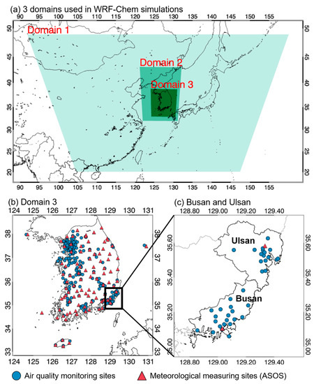
Figure 1.
Three domains used in the WRF-Chem simulations and the locations of monitoring and meteorological sites in the Busan and Ulsan metropolitan areas in southeastern Korea. (a), (b), and (c) represent the mother domain, first nested domain, and second nested domain of WRF-Chem model.
Meteorological observations within both the BMA and UMA were obtained from the KMA. Meteorological variables, including wind speed/direction, precipitation, cloud cover, and temperature were observed at the sites indicated in Figure 1, including a site located nearest to the sea in the BMA and the central urban site in the UMA. Air quality measurements, including hourly PM2.5 mass concentrations, were gathered from the air quality monitoring sites indicated in Figure 1, which are operated by the Korean Ministry of Environment (MOE). There are 18 air quality monitoring sites in BMA and 14 in UMA; these cover downtown, commercial, traffic, industrial, harbor, and residential areas. The observed PM2.5 concentration data were used to analyze the movement of polluted air and to compare against the simulated surface concentrations from WRF-Chem modeling.
WRF-Chem requires hourly, gridded, and speciated VOC emissions as an input data. The latest version of the Comprehensive Regional Emissions for Atmospheric Transport Experiment-2015 (CREATE-2015) emissions dataset was used in this study. The anthropogenic emissions of sulfur dioxide (SO2), nitrogen oxides (NOX), carbon monoxide (CO), VOCs, black carbon (BC), organic carbon (OC), PM10, and PM2.5 were based on the CREATE-2015 emission data. CREATE-2015 includes the Multi-resolution Emission Inventory of China (MEIC) [49], Clean Air Policy Support System (CAPSS) [50], and Regional Emission Inventory in Asia (REAS) version 2 [51]. Biogenic emissions were calculated online using a model based on the Model of Emissions of Gases and Aerosols from Nature (MEGAN) inventory [41]. MEGAN has been fully coupled into WRF-Chem to enable the online calculation of biogenic precursor emissions subject to vegetation cover and meteorological conditions such as temperature and solar radiation at the time of the calculation [47]. Dust, sea salt, and dimethyl sulfide (DMS) emissions were not included in this study.
4. Case Description
As a case study, we focused on the heat wave advisory days with no consecutive precipitation days under stagnant synoptic condition, and the heat wave alert/warning period was carefully selected. We analyzed the meteorological features and PM2.5 concentrations observed during the case study period and compared them with those observed over the last four years (from 2015 to 2018, since PM2.5 concentration data has been officially collected from January 2015, in Korea).
Figure 2 shows the time series of daily mean PM2.5 concentrations for both the heat-wave alert and wet precipitation periods. We also denoted a period governed by a stationary front located over the Korean Peninsula, called the “Changma” period, from 2015 to 2018. Changma is generally observed in July and August over the Korean Peninsula with an immense amount of precipitation. Daily average concentrations exceeding 35 µg/m3 (the criterion for a PM2.5 ‘bad’ grade defined as unhealthy level by Korean operational air quality prediction agency) are highlighted in Figure 2. Shaded bars represent precipitation days, and the “Changma” period is indicated. As shown in Figure 2, the rainy period (Changma period) was much shorter in 2018 than in other years, and the number of precipitation days in July, 2018 was recorded to be much lower than that in normal years (Table 2). The black line in Figure 2 indicates the days of heat wave alerts/warnings. Large numbers of heat wave alerts/warnings were issued in both cities (Busan and Ulsan) in both 2016 and 2018, but they were more frequent and continuous in 2018 than in 2016 in both cities. In particular, heat wave alerts/warnings persisted for a month in both cities in 2018, which broke the record duration set in 1973 in Korea [10].
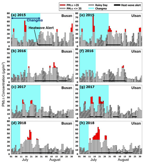
Figure 2.
Time series of daily mean PM2.5 concentrations and the durations of heat-wave alerts and the Changma period in July and August from 2015 to 2018 in both Busan and Ulsan metropolitan areas. (a)–(d) denote time series of PM2.5 with heat-wave alerts in 2015–2018 in Busan (left), and (e)–(h) in Ulsan (right), respectively.
Table 2.
Monthly mean PM2.5 concentrations and the number of days when the daily mean PM2.5 concentrations were higher than 35µg/m3 (Unhealthy) during June, July, and August from 2015 to 2018 for the Busan and Ulsan metropolitan areas, Korea.
In this regard, the period from 12 to 21 July 2018 was selected as a case study period (indicated in Figure 3) during which a heat-wave alert was consecutively issued with no precipitation under stagnant synoptic atmospheric conditions. As shown in Figure 3, a center of high pressure continuously overlaid the Korean Peninsula during the study period, and these stagnant atmospheric conditions offered sufficient circumstances to cause the accumulation of locally emitted pollutants and to generate secondary pollution.
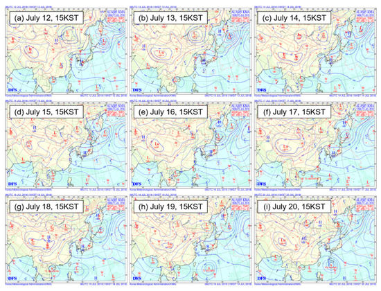
Figure 3.
850 hPa geopotential height field at 15KST 12–20 July 2018, denoted in (a)–(i), over East Asia.
The sensitivity of secondary aerosol formation depends on both atmospheric NOx and VOC emissions. In a previous study, NOx emission evaluation was reported [52] during the Korea-US Air quality (KORUS-AQ) Campaign based on a top-down assessment using an ozone monitoring instrument (OMI) whereby NO2 suggested an underestimation of 53% during the WRF-Chem simulations (NOx emissions by a factor of 2.13). In addition to Goldberg et al., [52], due to the remaining uncertainties, Miyazaki et al., [53] suggested the possibility of underestimation of NO2 emission when using top-down approaches, despite employing spatially more continuous and temporally more frequent data than bottom-up approach. However, anthropogenic VOC emission evaluation and OA generation from anthropogenic VOC emissions are poorly understood in modeling studies [54,55,56,57,58]. VOC emission evaluation has been attempted in several studies [54,55] by employing the diagnostics modeling through analyzing the discrepancies between modeled and observed concentrations. This process is of great importance for model performance because SOA formation is associated with VOC emissions and is known to be enhanced by active photochemical reaction conditions under high temperature, which leads to an increase in PM2.5 concentrations.
In this study, as the scaling factor for NOx emission has been applied in CREATE-2015 emission inventory, we only conducted VOC emission sensitivity study because the uncertainty of VOCs likely remains high, especially during heat wave alert periods such as the current heat-wave study period. For a better investigation of the impact of VOC on the secondary formation of PM2.5 during the heat wave period, three more experiments were conducted: doubling, five-fold increase, and ten-fold increase of VOC emission, in addition to a control experiment. This is because the effects of high temperature on SOA generations have not been quantified, and thus VOCs-related chemical mechanism is enhanced via active photochemical reaction under high temperature during the heat-wave period. Here, the relationship between VOC emissions and their sensitivity to the generation of SOA was investigated in the BMA and UMA in Korea when the temperature was highly elevated.
5. Sensitivity Simulations of VOC Emission and SOA Generation
In the BMA and UMA, one of the major uncertainties is the lack of knowledge on the source distributions of disaggregated VOC emissions, partly because of the numerous species of VOCs and their diverse origins. Therefore, sensitivity simulations were designed and executed to investigate potential causes of model biases in VOC emissions. When independent evidence of model performance evaluation is not readily available, these sensitivity tests are good tools for diagnosing model performance on which inputs affect model results and what magnitude of input adjustment can reduce discrepancies between model results and observations.
Multiple WRF-Chem simulations were carried out for the period covering 5–21 July 2018 with 7 days as a spin-up period, with a base case (CASE 1) and three more sensitivity tests doubling (twofold increase), quintupling (fivefold increase), and decupling (tenfold increase) the VOC emissions (CASE 2–CASE 4), respectively. Analyzing the differences between the four cases facilitates a diagnosis of the optimal VOC emissions under atmospheric conditions relevant to the BMA and UMA areas. CASE 4 with decupling (tenfold increase) the VOC scaling can be regarded as an extreme case of VOC enhancement from heat wave effects. Using these four WRF-Chem simulations, the enhanced PM2.5 concentrations were evaluated and the potential contribution of heat wave phenomena to PM2.5 formations over the BMA and UMA in Korea was explored.
Over the selected study period, modeling was carried out with the various emissions to specifically diagnose the impact of the heat wave. The WRF-Chem simulation was run for 433 h, with the first 7 days (168 h) discarded as model spin-up for meteorology–chemistry interactions during this period. As a result, this study was based on the assumption that the emission of precursors increased, and the photochemical reaction conditions led to an increase in the secondary generation of O3 and PM2.5 concentrations.
6. Results and Discussion
An overview of the monthly mean PM2.5 concentrations and the number of days with daily mean PM2.5 concentrations higher than 35 µg/m3 (unhealthy grade in the PM2.5 forecasting system in Korea) are listed in Table 2, for June, July, and August from 2015 to 2018 in the two cities. The differences in concentration between years were not obvious for the four years in both cities, but the occurrence of days exceeding 35 µg/m3 PM2.5 was higher in both 2015 and 2018 for Busan and Ulsan. Hourly maximum PM2.5 concentrations were highest in both 2015 and 2018. In 2015, 1-h maximum PM2.5 concentrations were 74.8 µg/m3 and 83.2 µg/m3 for Busan and Ulsan, and 72.8 µg/m3 and 84.2 µg/m3 for Busan and Ulsan, respectively, in 2018. We investigated the seasonal characteristics of backward trajectories and synoptic weather chart (not shown here) and found out that frequent long-range transport (LRT) processes dominated, originating from China inland, and extremely high PM2.5 were frequently observed in 2015. On the contrary, in 2018, our high episodic case during heat wave period occurred under consecutive stagnant synoptic conditions without LRT contributions, indicating short-term peaks in two areas were correlate well with the heat-wave alert period.
In order to find out the weather features during our high episodic cases, we investigated the synoptic situations at the 850 hPa level over the Korea Peninsula for the period from July 12 to July 20 (see Figure 3). The two cities were dominated by a long-lasting stagnant high-pressure system during the whole study period, as indicated in Figure 3. Therefore, these synoptic conditions with a weak prevailing wind speed made it possible for local circulations to develop within the two metropolitan areas, suggesting that the local air pollutants could be well characterized without transportation from other regions during the study period. Therefore, this study period provides good meteorological conditions to examine the accumulated air pollutants originating from local emissions and the generation process of secondary pollutants.
The time series of simulated and observed daily mean PM2.5 concentrations and meteorological variables in the two metropolitan areas were given in Figure 4, during the study period from 12 to 22 July 2018. As described above, meteorological conditions during the study period showed low wind speeds (which favored accumulation of PM2.5), high temperatures with a daily mean over 25 °C, and consecutive no-precipitation days with little or no cloud cover compared with other days in July, 2018. Overall, with the exception of small decreases on 16 and 18 July 2018, daily mean PM2.5 concentrations increased steadily from 12 to 19 July 2018; this may be related to the influence of accumulated air pollutants. We selected the period from 00:00 LST 12 July 2018 (15:00 UTC 11 July) to 00:00 LST 21 July 2018 (15:00 UTC 20 July) to examine, in detail, the impact of the heat wave period under long-lasting stagnant atmospheric conditions over both the BMA and UMA.
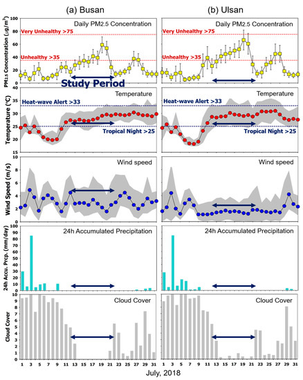
Figure 4.
Time series of observed daily mean PM2.5 concentrations and meteorological variables in July 2018 in Busan and Ulsan. Shaded areas represent the maximum and minimum of each variable. Also shown are observations in (a) Busan (left), and (b) Ulsan (right), respectively.
Before analyzing the air quality simulation results, we evaluated the performance of the WRF meteorological model. This study focused on the impact of high temperature on secondarily generated air pollutants during the heat wave period; therefore, we compared simulated temperatures against actual temperature observations. Figure 5 shows the time series of hourly observed and simulated temperatures, and scatter plots of simulations versus observations in the cities. As shown in Figure 5, the observed daily average temperatures were 27.99 °C (in Busan) and 29.14 °C (in Ulsan) for 12–21 July 2018, and the simulated temperatures were 27.75 °C (in Busan) and 29.71 °C (in Ulsan). These were similar to the observations during the same period (Figure 5). We also employed statistical parameters such as the correlation coefficient (R) and index of agreement (IOA), which are widely used to analyze model performance. High R values of 0.88 and 0.95 were found for Busan and Ulsan, respectively, indicating low discrepancies between observations and simulations (Figure 5). Wind speed and relative humidity showed R values of 0.77 and 0.82 for Busan, and 0.65 and 0.76 in Ulsan.
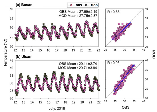
Figure 5.
Time series and scatter diagrams of hourly temperature from both observations and model simulations during the study period in Busan and Ulsan metropolitan areas. Also shown are time series and scatter diagrams for (a) Busan (top), and (b) Ulsan (bottom), respectively.
Figure 6 shows the time series of the observed PM2.5 concentrations and four simulated PM2.5 concentrations in Busan and Ulsan, and Table 3 provides a statistical summary of model performance for the latter. Busan had the highest R (0.83) and IOA (0.86) in CASE 4, whereas Ulsan had the highest R (0.75) and IOA (0.78) in CASE 3. These results indicate that the appropriate increase in VOCs was different for each region, and imply that scaling approximately by a factor of 5 may give the best PM2.5 simulation results. Elevated ozone was also simulated reasonably in CASE 3, showing that the maximum hourly O3 concentrations is elevated up to approximately 100 ppb that is very close to the observation (max. 108 ppb) (not shown here). Thus, VOC emissions in the BMA and UMA may be underestimated by factors of more or less than five in the two cities. In terms of the root mean squared error (RMSE), normalized mean bias (NMB), and mean bias error (MBE), CASE 4 was found to be the most appropriate simulation of the lower NMB for Busan, within ± 30%, according to the criteria suggested by Emery et al. [59]. In the case of Ulsan, CASE 3 was found to be the best simulation, implying a VOC emission scaling factor of more than five for the simulation of PM2.5 under heat-wave period emissions. We also analyzed the scatter diagrams of PM2.5 concentrations from the four sensitivity tests of the WRF-Chem simulations for both areas in Korea. The results indicated that CASE 4 is shown to best fit the y = x line for Busan (y = 1.1986x − 11.6723), and CASE 3 fits best for Ulsan (y = 1.0446x − 10.4250), corresponding well with the observed results indicated in Figure 6 and Table 3.
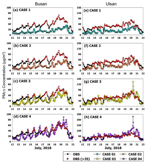
Figure 6.
Comparison of hourly PM2.5 concentrations from four sensitivity tests of WRF-Chem modeling and observation data in Busan and Ulsan metropolitan areas. (a)–(d) are results from CASE 1 to CASE 4 for Busan, and (e)–(h) for Ulsan, respectively.
Table 3.
Summary of paired comparisons for PM2.5 concentrations in Busan and Ulsan, Korea.
Figure 7 represents the time series of the anomalies of mass concentrations of PM2.5 for best fitted case during the study period, and the variations showed that the increase in VOC emissions resulted in day-time mass concentrations with peak time with the exception of 20 July 2018, but bias showed ranges less than 1 µg/m3 with the remarkable agreement of IOA (0.94) and RMSE (0.179).
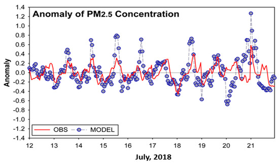
Figure 7.
Anomalies of PM2.5 concentrations from sensitivity tests of WRF-Chem modeling and observation data in Busan and Ulsan metropolitan areas.
The chemical components during the heat wave episodes and their differences to the non-heat wave period are also important characteristics associated with SOA formation. We therefore contrasted the model results between four cases in two cities. Figure 8 illustrates the simulated chemical components for each of the four cases. As shown in Figure 8, SOA formation became active as VOC emissions increased, and their mass concentration was simulated to increase accordingly. It is also interesting that the increase in VOCs did not necessarily increase SOA generation in a linear manner, but increased it by only 30% even when VOC emissions increased by a factor of 10. Nevertheless, the proportions of SOAs during this period were 42.3–66.6% (in Busan) and 34.3–56.6% (in Ulsan) for the four cases. As no measurements of chemical components were available, we could not compare the model results directly with observations. Therefore, further monitoring and modeling studies are needed for the diagnosis over the two cities in Korea.
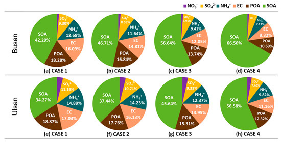
Figure 8.
Pie charts of chemical compositions of simulated PM2.5 concentrations for four simulations in Busan and Ulsan metropolitan areas. (a)–(d) are results from Busan (top), and (e)–(h) from Ulsan (bottom), respectively.
It is widely known that higher ratios of PM2.5/PM10 are induced by photochemical reactions originating from anthropogenic sources, whereas smaller PM2.5/PM10 ratios result from the generation of large particles predominantly by natural emissions [60,61]. According to the Busan Air Quality Assessment Report [62], the annual PM ratio in Busan ranged from 0.5 to 0.6 throughout the whole year, which contrasts with the current WRF-Chem results during the study period. We investigated the PM2.5/PM10 ratios simulated during the heat wave episodes. The time series of ratios of PM2.5 to PM10 for the four simulations in the two metropolitan areas are shown in Figure 9. In both areas, the PM2.5 to PM10 ratios were about 60% (min. scenario) to 92% (max. scenario). CASE 4, which showed the best model performances, averaged about 71% and 78%, with maxima of 91% and 92% in the two cities, respectively. On 19–20 July, the PM2.5 to PM10 ratio reached a maximum of 91–92% when the highest PM2.5 concentration was simulated with the highest temperature in Ulsan (and second highest temperature in Busan) during the study period. It was therefore inferred that photochemical reactions were most active on 20 July, 2018, driven by the high temperature, and actively generated SOA during the heat wave period in 2018.
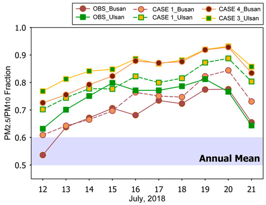
Figure 9.
Time series of ratios of PM2.5 to PM10 for CASE 1, the best case for each region, and observations in the Busan and Ulsan metropolitan areas.
Considering these simulated PM2.5/PM10 ratios, both the BMA and UMA tended to show considerably higher fractions during the heat wave period, compared with other season or previous years. Furthermore, the fraction increased overall as temperature increased, and the highest fraction occurred on 20 July, the day with the highest temperature and highest PM2.5 concentrations during the study period. Thus, these results strongly suggest that the notably high fraction was induced during the heat wave period when extremely high temperatures were observed in these urban areas of Korea.
In order to investigate the possible relationship between temperature vs. VOC emission, we further carried out the same sensitivity tests for non-heat wave periods; pre- and post- heat wave period (refer to as pre-HWP and post-HWP hereafter) during the entire summer season in 2018. We defined the period of 12–21 July as HWP, 1 June–11 July as pre-HWP, and 22 July–31 August as post-HWP, respectively, and the same scaled VOC emission applied by a factor of five was considered. The simulated SOA concentrations were all examined and inter-compared for three different periods.
The calculated mean differences (MD = OBS (avg) − Model (avg)) of SOA over each of the three periods were 8.84 µg/m3, 9.40 µg/m3, and 9.29 µg/m3, for pre-HWP, HWP, and post-HWP, in Busan, and 3.97 µg/m3, 2.56 µg/m3, and 5.57 µg/m3, in Ulsan, respectively. The averaged concentrations for two non-heat wave periods: pre- and post-HWP, were 9.06 µg/m3 (for Busan) and 4.79 µg/m3 (for Ulsan), and the differences between heat wave and non-heat wave period were about 1.47 µg/m3 (for Busan) and 2.24 µg/m3 (for Ulsan), respectively. The differences in our results appeared due to the higher emissions influenced by higher temperature during the heat wave period. Our assumption is that the emission of precursors was increased during the record-breaking period, and photochemical reaction conditions were enhanced as well, which elevated the probability of high PM2.5 concentrations. For example, the anthropogenic emission of VOCs is believed to be enhanced under the hot weather condition because of its variability: as the temperature increases, anthropogenic VOC’s emissions will increase. It appears, in this study, that the emission of anthropogenic VOCs is enhanced by high temperatures via both anthropogenic and natural processes. However, in our comparative simulation results between three different periods, namely heat wave, pre- and post-heat wave periods, it is also difficult to quantify these differences with specific factors, partly because of the differences in weather conditions such as precipitation, atmospheric boundary layers, and atmospheric stabilities in each of the three periods. It is also doubtful how significant these differences of simulated SOA formations were between three periods. In this respect, it seems difficult to determine this conclusion with our result alone.
It seems unlikely that we are able to draw a robust relationship with our result alone between increase in temperature vs. precursor’s emissions of PM2.5. One of the major difficulties is that we are unable to differentiate clearly between temperature effects and scaling effects from the underestimated VOCs emissions. Therefore, we are not suggesting that anthropogenic VOC emissions will clearly increase as the temperature increases. Instead, the changes in secondary PM2.5 concentrations were given via sensitivity simulations of the actual heat wave period, particularly focusing on interpreting the contributions of disaggregated VOCs to the enhancement of SOA over the main cities in southeast Korea.
7. Summary
The BMA and UMA experienced an unprecedented heat wave during 11 July–15 August, 2018, shortly after the “Changma” rainy season. During this period, PM2.5 concentrations were significantly elevated in the two metropolitan areas, with higher temperatures and weaker wind speeds than before and after the study period. The daily average PM2.5 concentrations observed during the period in both the BMA and UMA mostly exceeded 135 µg/m3 in Ulsan.
To analyze the effects of the heat wave on secondarily generated PM2.5 concentrations during the study period, we carried out analysis of both measurements and simulations. As a modeling study, we employed WRF-Chem to simulate PM2.5 concentrations and CREATE-2015 emissions over the BMA and UMA. As there were no robust VOC emission data for these extremely high temperature conditions, VOC emissions were determined and adjusted by carrying out several sensitivity simulations. Based on these “sensitivity run and adjustment” approaches, we evaluated the enhanced PM2.5 concentrations and explored the potential contribution of heat wave phenomena to PM2.5 secondary formations through photochemical reactions over the BMA and UMA in southern Korea.
The results showed that VOC emissions in the BMA and UMA were underestimated approximately by factors of five by CREATE-2015, and it was suggested that a considerable factor for scaling of VOC emission of CREATE-2015 yielded reasonable PM2.5 simulations for the heat wave period in the BMA and UMA. The simulated PM2.5 mass concentrations were compared with observations from the last four years, and it was concluded that the observed and simulated PM2.5 increased mainly because of photochemical reactions in these southern urban cities during the heat wave period in Korea. The simulated chemical components of PM2.5, SO42−, NH4+, OC, EC, POA, and SOA, showed increases during the study period, and the SOA components were most dominantly (but not linearly) enhanced as VOC emissions increased during the heat wave period.
The PM2.5 to PM10 ratios were about 74% (min. scenario) to 86% (max. scenario), with averages of 69% and 74% in Busan and Ulsan, respectively. The PM2.5 to PM10 ratio reached a maximum of 89%, when the highest PM2.5 concentrations were simulated with the highest temperature in Ulsan (and second highest temperature in Busan) during the study period. This suggested that photochemical reactions mostly induced the generation of SOAs during the heat wave in 2018. Considering the general ratios of PM2.5/PM10 reported by the Busan Air Quality Assessment Report [62], the annual mean ratios in Busan ranged from 0.5 to 0.6, contrasting considerably with the high PM2.5/PM10 ratios seen during the study period. During the study period, the ratios of PM2.5/PM10 increased as temperature increased, and the highest fraction occurred on the day with the highest temperature and the highest PM2.5 concentrations. These results suggest that extremely high temperatures with no precipitation are of significant importance in the secondary generation of PM2.5 masses in cities in southeastern Korea.
In addition, we further carried out the same sensitivity tests for non-heat wave periods, and investigated the possibility of anthropogenic VOC emissions influenced by higher temperature during the heat wave period. We found a small but detectable effect from our simulations. With these limited simulations carried out in our study alone, we are not suggesting the most-likely possibility of higher-than-normal anthropogenic VOC emission strengths partly originating from extremely high temperature, but it can be a potential relation between them, particularly around industrial areas such as Ulsan metropolitan area. As a future research, a highly complicated and well-designed intensive air quality monitoring campaign would be a prerequisite for this purpose. Together, more complicated sensitivities of changes in temperature to biogenic emissions should also be addressed over the areas in southeast Korea.
Author Contributions
Data curation, Y.-J.J.; Funding acquisition, C.-K.S.; Investigation, H.-J.L.; Writing―original draft, G.-H.Y.; Writing―review & editing, C.-H.K. All authors have read and agreed to the published version of the manuscript.
Funding
This research was funded by the National Strategic Project-Fine Particle of the National Research Foundation of Korea (NRF-2017M3D8A1092021) funded by the Ministry of Science and ICT (MSIT), the Ministry of Environment (ME), and the Ministry of Health and Welfare (MOHW).
Acknowledgments
The authors are grateful to two anonymous reviewers for their valuable comments.
Conflicts of Interest
The authors declare no conflict of interest.
References
- Saliba, N.A.; Kouyoumdjian, H.; Roumie, M. Effect of local and long-range transport emissions on the elemental composition of PM10–2.5 and PM2.5 in Beirut. Atmos. Environ. 2007, 41, 6497–6509. [Google Scholar] [CrossRef]
- Squizzato, S.; Masiol, M.; Innocente, E.; Pecorari, E.; Rampazzo, G.; Pavoni, B. A procedure to assess local and long-range transport contributions to PM2.5 and secondary inorganic aerosol. J. Aerosol Sci. 2012, 46, 64–76. [Google Scholar] [CrossRef]
- Wang, L.; Liu, Z.; Sun, Y.; Ji, D.; Wang, Y. Long-range transport and regional sources of PM2.5 in Beijing based on long-term observations from 2005 to 2010. Atmos. Res. 2015, 157, 37–48. [Google Scholar] [CrossRef]
- Sun, Y.; Zhuang, G.; Tang, A.; Wang, Y.; An, Z. Chemical characteristics of PM2.5 and PM10 in haze−fog episodes in Beijing. Environ. Sci. Technol. 2006, 40, 3148–3155. [Google Scholar] [CrossRef]
- Zhao, X.J.; Zhao, P.S.; Xu, J.; Meng, W.; Pu, W.W.; Dong, F.; He, D.; Shi, Q.F. Analysis of a winter regional haze event and its formation mechanism in the North China Plain. Atmos. Chem. Phys. 2013, 13, 5685–5696. [Google Scholar] [CrossRef]
- Wakamatsu, S.; Uno, I.; Suzuki, M. A field study of photochemical smog formation under stagnant meteorological conditions. Atmos. Environ. Part A Gen. Top. 1990, 24, 1037–1050. [Google Scholar] [CrossRef]
- Tai, A.P.; Mickley, L.J.; Jacob, D.J. Correlations between fine particulate matter (PM2.5) and meteorological variables in the United States: Implications for the sensitivity of PM2.5 to climate change. Atmos. Environ. 2010, 44, 3976–3984. [Google Scholar] [CrossRef]
- Wang, D.; Zhou, B.; Fu, Q.; Zhao, Q.; Zhang, Q.; Chen, J.; Yang, X.; Duan, Y.; Li, J. Intense secondary aerosol formation due to strong atmospheric photochemical reactions in summer: Observations at a rural site in eastern Yangtze River Delta of China. Sci. Total Environ. 2016, 571, 1454–1466. [Google Scholar] [CrossRef]
- Sun, J.; Gong, J.; Zhou, J.; Liu, J.; Liang, J. Analysis of PM2.5 pollution episodes in Beijing from 2014 to 2017: Classification, interannual variations and associations with meteorological features. Atmos. Environ. 2019, 213, 384–394. [Google Scholar] [CrossRef]
- KMA (Korea Meteorological Administration). Press Release. 2018. Available online: http://www.kma.go.kr/notify/press/kma_list.jsp?bid=press&mode=view&num=1193585 (accessed on 17 August 2018).
- NIER (National Institute of Environmental Research). Annual Report of Air Quality in Korea, 2018; NIER: Incheon, Korea, 2019.
- Haagen-Smit, A.J. Chemistry and physiology of Los Angeles smog. Ind. Eng. Chem. 1952, 44, 1342–1346. [Google Scholar] [CrossRef]
- Filella, I.; Penuelas, J. Daily, weekly and seasonal relationships among VOCs, NOx x and O3 in a semi-urban area near Barcelona. J. Atmos. Chem. 2006, 54, 189–201. [Google Scholar] [CrossRef]
- Wang, Q.G.; Han, Z.; Wang, T.; Zhang, R. Impacts of biogenic emissions of VOC and NOx on tropospheric ozone during summertime in eastern China. Sci. Total Environ. 2008, 395, 41–49. [Google Scholar] [CrossRef] [PubMed]
- Duncan, B.N.; Yoshida, Y.; Olson, J.R.; Sillman, S.; Martin, R.V.; Lamsal, L.; Hu, Y.; Pickering, K.E.; Retscher, C.; Allen, D.J.; et al. Application of OMI observations to a space-based indicator of NOx and VOC controls on surface ozone formation. Atmos. Environ. 2010, 44, 2213–2223. [Google Scholar] [CrossRef]
- Tan, Z.; Lu, K.; Jiang, M.; Su, R.; Dong, H.; Zeng, L.; Zhang, Y. Exploring ozone pollution in Chengdu, southwestern China: A case study from radical chemistry to O3-VOC-NOx sensitivity. Sci. Total Environ. 2018, 636, 775–786. [Google Scholar] [CrossRef] [PubMed]
- Guenther, A.B.; Monson, R.K.; Fall, R. Isoprene and monoterpene emission rate variability: Observations with eucalyptus and emission rate algorithm development. J. Geophys. Res. Atmos. 1991, 96, 10799–10808. [Google Scholar] [CrossRef]
- Guenther, A.B.; Zimmerman, P.R.; Harley, P.C.; Monson, R.K.; Fall, R. Isoprene and monoterpene emission rate variability: Model evaluations and sensitivity analyses. J. Geophys. Res. Atmos. 1993, 98, 12609–12617. [Google Scholar] [CrossRef]
- Geron, C.; Guenther, A.; Greenberg, J.; Loescher, H.W.; Clark, D.; Baker, B. Biogenic volatile organic compound emissions from a lowland tropical wet forest in Costa Rica. Atmos. Environ. 2002, 36, 3793–3802. [Google Scholar] [CrossRef]
- Geron, C.; Guenther, A.; Greenberg, J.; Karl, T.; Rasmussen, R. Biogenic volatile organic compound emissions from desert vegetation of the Southwestern US. Atmos. Environ. 2006, 40, 1645–1660. [Google Scholar] [CrossRef]
- Churkina, G.; Kuik, F.; Bonn, B.; Lauer, A.; Grote, R.; Tomiak, K.; Butler, T.M. Effect of VOC Emissions from Vegetation on Air Quality in Berlin during a Heatwave. Environ. Sci. Technol. 2017, 51, 6120–6130. [Google Scholar] [CrossRef]
- Tunved, P.; Hansson, H.-C.; Kerminen, V.-M.; Ström, J.; Dal Maso, M.; Lihavainen, H.; Viisanen, Y.; Aalto, P.P.; Komppula, M.; Kulmala, M. High Natural Aerosol Loading over Boreal Forests. Science 2006, 312, 261–263. [Google Scholar] [CrossRef]
- Hodzic, A.; Jimenez, J.L.; Madronich, S.; Aiken, A.C.; Bessagnet, B.; Curci, G.; Fast, J.; Lamarque, J.-F.; Onasch, T.B.; Roux, G.; et al. Modeling organic aerosols during MILAGRO: Importance of biogenic secondary organic aerosols. Atmos. Chem. Phys. 2009, 9, 6949–6981. [Google Scholar] [CrossRef]
- Chen, Q.; Farmer, D.K.; Schneider, J.; Zorn, S.R.; Heald, C.L.; Karl, T.G.; Guenther, A.; Allan, J.D.; Robinson, N.; Coe, H.; et al. Mass Spectral Characterization of Submicron Biogenic Organic Particles in the Amazon Basin. Geophys. Res. Lett. 2009, 36, L20806. [Google Scholar] [CrossRef]
- Slowik, J.G.; Stroud, C.; Bottenheim, J.W.; Brickell, P.C.; Chang, R.Y.-W.; Liggio, J.; Makar, P.A.; Martin, R.V.; Moran, M.D.; Shantz, N.C.; et al. Characterization of a large biogenic secondary organic aerosol event from eastern Canadian forests. Atmos. Chem. Phys. 2010, 10, 2825–2845. [Google Scholar] [CrossRef]
- Nault, B.A.; Campuzano-Jost, P.; Day, D.A.; Schroder, J.C.; Anderson, B.; Beyersdorf, A.J.; Blake, D.R.; Brune, W.H.; Choi, Y.; Corr, C.A.; et al. Secondary organic aerosol production from local emissions dominates the organic aerosol budget over Seoul, South Korea, during KORUS-AQ. Atmos. Chem. Phys. 2018, 18, 17769–17800. [Google Scholar] [CrossRef]
- Heald, P.C.; Schladow, S.G.; Allen, B.C.; Reuter, J.E. VOC Loading from Marine Engines to a Multiple–use Lake. Lake Reserv. Manag. 2005, 21, 30–38. [Google Scholar] [CrossRef]
- De Gouw, J.A.; Middlebrook, A.M.; Warneke, C.; Goldan, P.D.; Kuster, W.C.; Roberts, J.M.; Fehsenfeld, F.C.; Worsnop, D.R.; Canagaratna, M.R.; Pszenny, A.A.; et al. Budget of organic carbon in a polluted atmosphere: Results from the New England Air Quality Study in 2002. J. Geophys. Res. Atmos. 2005, 110. [Google Scholar] [CrossRef]
- Volkamer, R.; Jimenez, J.L.; Martini, F.S.; Dzepina, K.; Zhang, Q.; Salcedo, D.; Molina, L.T.; Worsnop, D.R.; Molina, M.J. Secondary organic aerosol formation from anthropogenic air pollution: Rapid and higher than expected. Geophys. Res. Lett. 2006, 33, L17811. [Google Scholar] [CrossRef]
- Pun, B.K.; Seigneur, C. Investigative modeling of new pathways for secondary organic aerosol formation. Atmos. Chem. Phys. 2007, 7, 2199–2216. [Google Scholar] [CrossRef]
- Simpson, D.; Yttri, K.E.; Klimont, Z.; Kupiainen, K.; Caseiro, A.; Gelencsér, A.; Pio, C.; Puxbaum, H.; Legrand, M. Modeling carbonaceous aerosol over Europe: Analysis of the CARBOSOL and EMEP EC/OC Campaigns. J. Geophys. Res. Atmos. 2007, 112, D23S14. [Google Scholar] [CrossRef]
- Hodzic, A.; Jimenez, J.L.; Madronich, S.; Canagaratna, M.R.; DeCarlo, P.F.; Kleinman, L.; Fast, J. Modeling organic aerosols in a megacity: Potential contribution of semi-volatile and intermediate volatility primary organic compounds to secondary organic aerosol formation. Atmos. Chem. Phys. 2010, 10, 5491–5514. [Google Scholar] [CrossRef]
- Tsimpidi, A.P.; Karydis, V.A.; Zavala, M.; Lei, W.; Molina, L.; Ulbrich, I.M.; Jimenez, J.L.; Pandis, S.N. Evaluation of the volatility basis-set approach for the simulation of organic aerosol formation in the Mexico City metropolitan area. Atmos. Chem. Phys. 2010, 10, 525–546. [Google Scholar] [CrossRef]
- Rubin, J.I.; Kean, A.J.; Harley, R.A.; Millet, D.B.; Goldstein, A.H. Temperature dependence of volatile organic compound evaporative emissions from motor vehicles. J. Geophys. Res. Atmos. 2006, 111. [Google Scholar] [CrossRef]
- Faber, J.; Brodzik, K.; Łomankiewicz, D.; Gołda-Kopek, A.; Nowak, J.; Świątek, A. Temperature influence on air quality inside cabin of conditioned car. Combust. Engines 2012, 149, 49–56. [Google Scholar]
- Jacob, D.J.; Winner, D.A. Effect of Climate Change on Air Quality. Atmos. Environ. 2009, 43, 51–63. [Google Scholar] [CrossRef]
- Svendby, T.M.; Lazaridis, M.; Torseth, K. Temperature dependent secondary organic aerosol formation from terpenes and aromatics. J. Atmos. Chem. 2008, 59, 25–46. [Google Scholar] [CrossRef]
- Takekawa, H.; Minoura, H.; Yamazaki, S. Temperature dependence of Secondary Organic Aerosol formation by Photo-oxidation of hydrocarbons. Atmos. Environ. 2003, 37, 3413–3424. [Google Scholar] [CrossRef]
- Sheehan, P.E.; Bowman, F.M. Estimated effects of temperature on secondary organic aerosol concentrations. Environ. Sci. Technol. 2001, 35, 2129–2135. [Google Scholar] [CrossRef]
- Shon, Z.-H. Emissions of Ozone Precursors from a Biogenic Source and Port-related Sources in the Largest Port City of Busan, Korea. Asian J. Atmos. Environ. 2015, 9, 39–47. [Google Scholar] [CrossRef]
- Guenther, A.; Karl, T.; Harley, P.; Wiedinmyer, C.; Palmer, P.I.; Geron, C. Estimates of global terrestrial isoprene emissions using MEGAN (Model of Emissions of Gases and Aerosols from Nature). Atmos. Chem. Phys. 2006, 6, 3181–3210. [Google Scholar] [CrossRef]
- BMC (Busan Metropolitan City). 55th Busan Statistical Yearbook; BMC: Busan, Korea, 2017. [Google Scholar]
- MOE (Ministry of Environment). Environmental Statistics Yearbook; MOE: Seoul, Korea, 2018.
- UMC (Ulsan Metropolitan City). Statistical Yearbook; UMC: Ulsan, Korea, 2016. [Google Scholar]
- Oh, I.-B.; Kim, Y.-K. Surface Ozone in The Major Cities of Korea: Trends, Diurnal and Seasonal Variations, and Horizontal Distributions. J. Korean Soc. Atmos. Environ. 2002, 18, 253–264. [Google Scholar]
- Skamarock, W.C.; Klemp, J.B.; Dudhia, J.; Gill, D.O.; Barker, D.M.; Wang, W.; Powers, J.G. A Description of the Advanced Research WRF Version 3, NCAR/TN–475+STR NCAR TECHNICAL NOTE; Mesoscale and Microscale Meteorology Division, National Center of Atmospheric Research: University Park, PA, USA, 2008. [Google Scholar]
- Grell, G.A.; Peckham, S.E.; Schmitz, R.; McKeen, S.A.; Frost, G.; Skamarock, W.C.; Eder, B. Fully coupled “online” chemistry within the WRF model. Atmos. Environ. 2005, 39, 6957–6975. [Google Scholar] [CrossRef]
- Fast, J.D.; Gustafson, W.I., Jr.; Easter, R.C.; Zaveri, R.A.; Barnard, J.C.; Chapman, E.G.; Grell, G.A. Evolution of ozone, particulates, and aerosol direct forcing in an urban area using a new fully coupled meteorology, chemistry, and aerosol model. J. Geophys. Res. 2006, 111, D21305. [Google Scholar] [CrossRef]
- Multi-resolution Emission Inventory of China (MEIC). Available online: http://www.meicmodel.org/ (accessed on 27 January 2020).
- Clean Air Policy Support System (CAPSS). Available online: http://airemiss.nier.go.kr (accessed on 27 January 2020).
- Regional Emission Inventory in Asia (REAS) Version 2. Available online: http://www.jamstec.go.jp/frsgc/research/d4/emission.htm (accessed on 27 January 2020).
- Goldberg, D.L.; Saide, P.E.; Lamsal, L.N.; de Foy, B.; Lu, Z.; Woo, J.H.; Streets, D.G. A top-down assessment using OMI NO2 suggests an underestimate in the NOx emissions inventory in Seoul, South Korea, during KORUS-AQ. Atmos. Chem. Phys. 2019, 19, 1801–1818. [Google Scholar] [CrossRef]
- Miyazaki, K.; Eskes, H.J.; Sudo, K. Global NOx emission estimates derived from an assimilation of OMI tropospheric NO2 columns. Atmos. Chem. Phys. 2012, 12, 2263. [Google Scholar] [CrossRef]
- Wu, X.; Huang, W.; Zhang, Y.; Zheng, C.; Jiang, X.; Gao, X.; Cen, K. Characteristics and uncertainty of industrial VOCs emissions in China. Aerosol Air Qual. Res. 2015, 15, 1045–1058. [Google Scholar] [CrossRef]
- Kim, C.-H.; Park, S.-U.; Song, C.-K. A simple semi-empirical photochemical model for the simulation of ozone concentration in the Seoul metropolitan area in Korea. Atmos. Environ. 2005, 39, 5597–5607. [Google Scholar] [CrossRef]
- Kim, C.-H.; Kim, Y.-K.; Lee, H.W.; Seo, K.-H. A simple method for simulating horizontal ozone concentration fields over coastal areas: A case study of the Seoul metropolitan area, Korea. Terr. Atmos. Ocean. Sci. 2009, 20, 355–363. [Google Scholar] [CrossRef][Green Version]
- Kanakidou, M.; Seinfeld, J.H.; Pandis, S.N.; Barnes, I.; Dentener, F.J.; Facchini, M.C.; Van Dingenen, R.; Ervens, B.; Nenes, A.; Nielsen, C.J.; et al. Organic aerosol and global climate modelling: A review. Atmos. Chem. Phys. 2005, 5, 1053–1123. [Google Scholar] [CrossRef]
- Hallquist, M.; Wenger, J.C.; Baltensperger, U.; Rudich, Y.; Simpson, D.; Claeys, M.; Dommen, J.; Donahue, N.M.; George, C.; Goldstein, A.H.; et al. The formation, properties and impact of secondary organic aerosol: Current and emerging issues. Atmos. Chem. Phys. 2009, 9, 5155–5236. [Google Scholar] [CrossRef]
- Emery, C.; Liu, Z.; Russell, A.G.; Odman, M.T.; Yarwood, G.; Kumar, N. Recommendations on statistics and benchmarks to assess photochemical model performance. J. Air Waste Manag. Assoc. 2016, 67, 582–598. [Google Scholar] [CrossRef]
- Sugimoto, N.; Shimizu, A.; Matsui, I.; Nishikawa, M. A method for estimating the fraction of mineral dust in particulate matter using PM2.5-to-PM10 ratios. Particuology 2016, 28, 114–120. [Google Scholar] [CrossRef]
- Xu, G.; Jiao, L.; Zhang, B.; Zhao, S.; Yuan, M.; Gu, Y.; Liu, J.; Tang, X. Spatial and Temporal Variability of the PM2.5/PM10 Ratio in Wuhan, Central China. Aerosol Air Qual. Res. 2017, 17, 741–751. [Google Scholar] [CrossRef]
- BRI (Busan Research Institute). Annual Report of Air Pollution and Environment in Busan Metropolitan Area; BRI: Busan, Korea, 2019. [Google Scholar]


© 2020 by the authors. Licensee MDPI, Basel, Switzerland. This article is an open access article distributed under the terms and conditions of the Creative Commons Attribution (CC BY) license (http://creativecommons.org/licenses/by/4.0/).